The Algorithm Of Extracting Cyclographic Maps

全文

(1)THE ALGORITHM OF EXTRACTING CYCLOGRAPHIC MAPS. Ching-Shoei Chiang Computer and Information Science, Soochow University, Tappei, Taiwan, R.O.C. Email:chiang@cis.scu.edu.tw respectively, when the ∆t approaches to zero. Let p be a point on the oriented simple curve α, let θ be the angle measured counter-clockwise from p′s left tangent to its right tangent. If θ=0, the point p is a differentiable point. If 0<θ<π or π<θ<2π, the point is a convex or concave vertex respectively. There are two cases for θ=π. Consider the curve in Figure 1a and 1b, the point p separate the curve into two subcurves α1 and α2, α1 is from start point to p and α2 is from p to the end point. If α2 is locally in the “left-side” of α1 at p(Figure 1a), then p is a convex vertex. If α2 is locally in the “right-side” of α1 at p(Figure 1b), then p is a concave vertex. If α1 is locally equal to the α2, the curve α will not be simple. We only consider simple curve with bounded curvature variation in this paper.. ABSTRACT The cyclographic maps and its relation to offset curve, the medial axis transform is introduced in this paper. We also modify the cyclographic maps into the weighted cyclographic maps and extracting the weighted offset curves and weighted medial axis transform from it. Algorithm to extract the cyclographic map from the boundary curve is introduced. 1. Introduction – Offset Curve, Medial Axis Transform There are 4 sections in this paper. The first section gives definitions for the curve and the oriented curve, introduces r-offset of the (oriented) curve, medial axis and medial axis transform associated with “one side” of a curve, or a closed domain. The second section describes the cyclographic maps. The third section describes the algorithm of extracting cyclographics and weighted cyclographics for an oriented curve, and the final section describes the relationship between cyclographics and offset curve, medial axis transform, and blending curves.. α2. α1. α1. α2. left tangent right tangent. (a) Convex. left tangent right tangent. (b) Concave. Figure 1 Convex/concave with opposite tangent direction. 1.1 Curves Definition 1 A curve in the real Euclidean space R2 is a map α:[a,b]->R2, where α(t)=(x(t),y(t)) and x(t), y(t) are continuous functions. An oriented curve is a curve with orientation from α(a) to α(b).. The right normal vector and left normal vector are further defined as the right tangent and left tangent vectors which rotated 90 degree counter-clockwise. The negative left normal of α at p is the left normal with reverse direction. The negative right normal and the negative normal are defined similarly. There is no left and right normal for the start and end points of α respectively.. If is an oriented curve, we called the point α(a) and α(b) the start and end point of the oriented curve. If α is a curve, we called both α(a) and α(b) end points. Definition 2 A (oriented) curve α:[a,b]->R2 is:. Notice that for the differentiable point p, its left tangent is equal to its right tangent, and its left normal is equal to its right normal. We simply call them the tangent of p or the normal of p. We treat the start and end point are differentiable points. Their tangents (normals) are right tangent (normal) and left tangent (normal) respectively.. • simple if α is one-to-one. • differentiable if dα/dt is defined and not zero, for all t∈[a,b], where dα/dt is the derivative of α by t. • twice differentiable if d2α/d 2 is defined and not zero, for all t∈[a,b], where d2α/d 2 is the second derivative of α at t.. The left(right) side of the oriented simple curve α at p is defined as follows:. • closed if α(a)=α(b).. • If the point p is differentiable, the left(right) side of α at p is the normal(negative normal) of α at p.. • of bounded curvature variation if there are finitely many local extrema of the curvature. And, there are finitely many inflection points.. • If the point p is a convex point, the left(right) side of α at p is the area span by the vectors rotated counter-clockwise from the (negative) left normal at p to the (negative) right normal at p.. We define the right tangent and the left tangent of α(t) as the vector from α(t+∆t) to α(t) and from α( t-∆t) to α(t) 1.

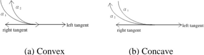
(2) • If the point p is a concave point, the left side of α at p is the area span by the vectors rotated clockwise from the (negative) left normal at p to the (negative) right normal at p.. distl+(q,α)={d(p,q) | p∈α; d(p,q) has exreme value; and q is on the left side of α at p}. • The left(right) side of an oriented simple curve α is the union of the left(right) side of α at all points on α.. distg+(q,α) = min { distl+(q,α)}. Notice that under these definitions, the left(right) side of an open oriented curve is not necessary bounded.. distl-(q,α)={-d(p,q)|p∈α; d(p,q) has exreme value; and q is on the right side of α at p} distg-(q,α) = max { distl-(q,α)}. 1.2 Offset Curves We introduce the notions of local distance, global distance, local offset and global offset in this section. Given a plane curve C, its offset by a distance r is a curve Off(C,r) such that the points of Off(C,r) are at distance r from C. These informal definitions can be made more precise in one of two ways, depending on whether the distance is measured locally or globally. Denote the Euclidean distance of two points p and q with d(p,q). Let C be a curve in R2, and p any point. Define the global distance of p to C by distg(p,C) = {d(p,q) | q ∈ C and d(p,q) has global minimal} where d(p,q) is the Euclidean distance of two points. For a smooth curve C, a local distance can be defined as distl (p,C) = {d(p,q) | q ∈ C and d(p,q) has extreme value} Notice that distg (p,C) = min { distl (p,C)} From [1], we know that if q is not end point of the curve C, and C is differential at q, then pq is perpendicular to the tangent of C at q. For most reasonable curves C these definitions make sense. Notice that distg (p,C) is a singleton and distl (p,C) may have more than one element. Given a parametric or implicit representation of the curve. the local and global offsets can be defined as follows2, 3,4]. In the global offset, the global distance is used, so that Offg(C,r) = { p∈ R2 | r ∈ distg(p,C) } Local offsets are simple to define analytically, That is, Offl(C,r) = { p∈ R2 | r ∈ distl(p,C) } Moreover, the local offset of an algebraic curve or surface again is an algebraic curve. Notice that the offset of a curve has two components for a curve, each one on the different side of the curve. We restricted the offset of an oriented curve to be the offset on its left side. 1.3 Offsets for an oriented simple curve Let us consider the offset for the oriented curve α. We give distance with sign on the oriented curve. For the point at the left(right) side of α at p, its distance to p is positive(negative). Notice that there exist points on both sides of α, as the point q in Figure 2. We call that p1 is q′s footpoint on α from q′s right side, and p2 is q′s footpoint on α from q′s left side. Or, q is on left side of α at p1, and q is on right side of α at p2. The local and global distance for point to oriented curve are defined as:. p2 r2<0 q. r1>0. p1. Figure 2 points on both sides of α Let’s consider the r-offset for an oriented simple curve now. If r>0(r<0), the r-offset of α is the trace of points that is in the left(right) side of the curve, and its distance to the curve is equal to r. This r-offset can be global or local, depend on the local global distance or local distance we use. Under this definition, if β is the same as α except that β is not oriented, the union for the r-offset and –r-offset of α is not equal to the r-offset of β. The only difference is at the start and end point of the curve α. The offset of contains circular arc at the start and end point, the r-offset of α is the intersection of r-offset of β and the left side of α. Similarly, the –r-offset of α is the intersection of r-offset of β and the right side of α. The local and global offsets of an oriented curve are defined as: Offg(α,r) = { p∈ R2 | r∈distg+(p,α) or r∈distg-(p,α) } Offl(α,r) = { p∈ R2 | r∈distl+(p,α) or r∈distl-(p,α) } In the above definition, if the point p is not on the left side and right side of α, we defined distl+(p,α) and distl-(p,α) are equal to ∞ and -∞ respectively. It is possible that a point is both on the positive and negative offset of α, as the point p in Figure 2. The point q is on both +r-offset and –r-offset of α. when r=r1=-r2. If C is the curve α without orientation, we have Offg(α,r)∈ Offg(C,|r|) Offl(α,r)∈ Offl(C,|r|) The proof is base on the fact that there are more restriction to define distg and distl for oriented curve than curve. Consider the curve C with the implicit equation f(x,y)=0. Let (u1,v1) be a point on f and (x,y) be a point on the normal of f at (u1,v1). Let fx denote the differential of f with respect to x. In 2D, the system of equation for the local offsets with distance d to the boundary in the dimensionality paradigm is 6]: f(u,v) = 0 fx(y-v) - fy(x-u) = 0 (x-u)2 + (y-v) 2 = d2 2.

(3) The first equation states that the point (u1,v1) is on f. The second equation assures the fact that (x,y) is on the normal of f at (u1,v1). And, the third equation asserts that the distance from the boundary curve to offset curve is equal to d. Notice that in the general case, the degree of freedom is 1, so that the offset of the curve should be a curve in 2D. With similar approach, we can generate the system of equation for the curve with parametric form. Consider the curve C(t)=((X(t),Y(t)), we have the following system of equation: (x-X(t))*Xt(t)+(y-Y(t))*Yt (t)=0 (x-X(t))2+(y-Y(t))2=d2 We can eliminate the variable to find the implicit form for the offset curve [22]. The properties of the 2D offset curves is well introduced in [24,25]. There are also many algorithms to extract 2D offsets, such as [26,27]. 1.4 Medial Axis and Medial Axis Transform 2. Consider a compact region in R . There are two equivalent definitions for the medial axis (MA) of such region, namely: Definition 3 (Blum) The internal medial axis (or skeleton) of a 2D compact region is the closure of the locus of the centers of all maximal disks which are contained in the shape. Definition 4 Let a footpoint of p be a point p' on the boundary of a 2D region that has minimum distance to p. The interior medial axis of a 2D closed region is the closure of the locus of the points inside the region which have more than one footpoint. Let’s extend the definition 4 into noncompact 2D region. Consider an oriented curve with it left side as the 2D region, the medial axis of this 2D region is the closure of the locus of the points inside the region which have more than one footpoint. Notice that under this definition, the line connect the point p with it footpoint p′ will perpendicular the the tangent of the boundary curve at p′. We can define the MAT+ and MAT- for oriented curve. The MAT+ of the oriented curve α is the closure of the set of points which located on right (left) of α and have two or more footpoints on α from their left (right). Consider the point q on Figure 2. Although q is on the left side of α (and also the right side of α), there are only one footpoint p1 on α from its right, so the point q is not belong to MAT+ of α. More formally, we have: MAT+(α)=closure{q | q is on the left side of α; q has more than one footpoints on α from q′s right side } MAT-(α)=closure{q | q is on the right side of α; q has more than one footpoints on α from q′s left side of α } The function which maps an MA point to the distance between the MA point and its footpoints is called the radius function. The medial axis and the associated radius function define the medial axis transform (MAT). The definition. extends naturally to the concept of an left(right) MAT associated to the left(right) side of an oriented curve. There are many applications of the MAT of 2D regions. The interior MAT can be used in shape representation and shape recognition [7,8,9,10,11,12], especially for objects whose width is relatively unimportant such as characters in character recognition, or chromosomes in microbiology. The medial axis has also been used in finite-element mesh generation [13,14,15,16]. Many global shape characteristics can be extracted from the internal MAT of the shape, as explained in [13]. The external MAT can be used in motion planning [17]. For example, the external MAT of n obstacles can be used to define a collision-free path for robots that maximizes clearance from the obstacles. The MAT is also useful in casting design [18] and has potential applications in geometric tolerancing [19]. The properties of 2D MAT can be find in [28, 30]. There are also many algorithms to extract 2D MAT, such as [28, 29]. 2. Cyclographics and Weighted Cyclographics Cyclographic maps has been introduced in [20] and used in computer science[19]. Every point in (x,y,z)-space is associated with an oriented circle in the (x,y)-plane by making the point the vertex of a double right cone whose axis is parallel to the z-axis and intersecting the cone with the (x,y)-plane. If the point has a z-coordinate grater than 0, the orientation of the circle is counterclockwise, otherwise, the orientation of the circle is clockwise. Consider an oriented curve C in 2D, and rotate all of its normals 45 degrees about the tangent. Then we obtained a ruled surface called the cyclographic map S(C) of C. The projection of the self-intersection points of the surface onto the (x,y)-plane contains the MA of the curve. The internal MA is produced on one side (the side with z value greater than 0) and the external MA on the other side(z<0). If we do not care about the orientation of the circles, we can think of the cyclographic maps in another way. Let D be a closed simple domain, and consider the single cones whose apex is on the boundary and whose axis is parallel to the z axis where the interior of the cone is in the z>0 region. Then, the envelope of the cones in the region z≥0 is a different new cyclographic map. The only difference is that the new map is in the positive z-half space. The MAT is obtained in the set of the self-intersection points of the envelope. The internal MAT and the external MAT are all on the same side of the (x,y)-plane. Consider all cones whose apex is on the MATand whose axis is parallel to z-axis. The union of all the circles that are the intersection of the cones with the (x,y)-plane are then the original domain D. The plane z=r intersections with the maps produce the local r-offset of the original domain. Notice that every point in the half space z≥0 corresponds to a right cone in 3D or a circle on (x,y)-plane, which means that three dimensional half-space can be representing by the set of circles in the plane. This notion that space could be treated as a collection of elements other than points was proposed by Plucker over 100 years ago 21]. We can restrict the surface S(C) such that it is the graph of a 3.

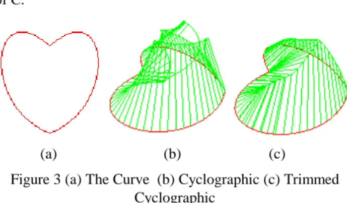
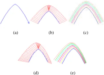
(4) function with the (x,y)-plane its domain. With each point (x,y), we associate the minimum |r|, so that the point (x,y,r) is on S(C). Let us call this surface the trimmed cyclographic map of C. The surface so defined is then the distance surface of Blum 7]. It follows, that the trimmed cyclographic map of C can be determined approximately with the Euclidean distance transform. Notice the trimmed cyclographic map of C can be obtained from the cyclographic map of C . The cyclographic map can be easily extended to any closed domain with an oriented curve as its boundary, such as domains with holes. Figure 3(b)(c) shown examples of the cyclographic map and the trimmed (modified) cyclographic of the boundary curve of Figure 3(a). Notice that the rotated normal of a differentiable point q∈C is a line for the cyclographic map of C and could be a line, half-line, or line segment for the trimmed cyclographic map of C.. 1. Input the boundary curve using the piecewise cubic Bezier curve Ci(t), 1≤ i ≤m. 2. Find n intermediate points pi,j,1≤j≤n+2, for each curve Ci(t) and each concave and concex vertex. Further, find the rotated normal for all of the point pi,j. Reorder the boundary point into a list Q=[qi]. The above algorithm produce the rotated normal of all boundary points, we can display the cyclographic maps easily from the boundary curve points associated with its rotated normal, as shown in Figure 3b. In order to find the trimmed cyclographic map, we have to find its self-intersection curve, and trim the cyclographic map. We use the divided and conquer strategy as the following: Algorithm 2: Trimmed Cyclograhpic Maps 1. Input the boundary curve using the piecewise cubic Bezier curve Ci(t) , 1≤ i ≤m. 2. Find n intermediate points pi,j for each curve Ci(t) and each concave and concave vertex. Furthermore, find the rotated normal for all of the point pi,j. Reorder all of the boundary points into a list Q=[qi].. (a). (b). (c). Figure 3 (a) The Curve (b) Cyclographic (c) Trimmed Cyclographic In the cyclographic map, every rotated normal has 45 degree with z=0 plane. The weighted cyclographic map is defined similar to cyclographic except that the degree between the rotated normal and z=0 are varied. We define the degree function w(t) be the degree of the rotated normal along the oriented curve with z=0 plane. We use the similar way to define the trimmed weighted Cyclographic maps. The weighted local (global) r-offset curve is defined as the intersection of z=r plane with weighted (trimmed weighted) cyclographic maps. The weighted MAT of the left region of an oriented curve is obtained in the self-intersection of its rotated normals. 2.Algorithm for extracting Cyclographic maps of oriented curve We describe the algorithm which extracting cyclographic maps of oriented curve in this section. Given a closed bounded domain, we would like to produce its trimmed cyclographic maps, so that the global weighted offsets of the boundary curve, weighted MAT of this closed domains, etc., can be easy extract from the cyclographic maps. The boundary curve is represented by a list of the boundary point with its associated rotated normals. We generated the cyclographic maps via two algorithms. The first one produce the cyclographic map and the second one produce the trimmed cyclographic map. Algorhthm 1: Cyclotraphic map. 3. Let q2 as the starting boundary point, find its associated MAT point q and q′s other footpoints. If the other footpoints is not one of qj, j≠i, and between qi and qi+1, then we insert one more boundary point qk between qi and qi+1 with its rotated normal in the list of points Q. 4. Separate the list Q into two (or more, if the first MAT points we find is a branch point) lists via the MAT point q and its footpoints q2 and qk. 5. Push all of the lists into a queue. 6. If the queue is empty, go to 9. Otherwise, pop a list from queue. March along the MAT curve via the lists of points and associated MAT curve. Mark the boundary points after visit the boundary point. 7. If the MAT curve hit a branch point, subdivide the domain (point list) into three or more subdomains (point lists). Go to 5. 8. If the MAT curve hit an end point, go to 6. 9. Stop. After the above algorithm, every rotated normal is bounded by an MAT point. The trimmed cyclographic maps is also easy to display, as shown in Figure 3c. Notice that the trimmed cyclographic maps produce extra boundary points in the third step in Algorithm 2, as we can see in the figure. Notice also that if we modify the algorithm, so that the rotated normal is a line instead of vector, and trim the rotated normal on both side, we can produce not only the internal MAT but also external MAT. We answer the following questions steps by steps: 1. How to find the associated MAT and other footpoints (Step 3)? Let q2 as the starting boundary point, We would like to find 4.

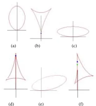
(5) its associated MAT point q and other footpoints. Consider the rotated normal of q2 and other rotated nromals. Two consequence points with its rotated normal produce a bilinear surface. Because this two points are closed to each other, we can use a plane P to approximate the bilinear surface. If the rotated normal of q2 intersect the plane P, then there is a MAT point on the plane P, we would like to find the intersection of the rotated normal of q2 and the plane P. Sometimes there are more one such plane, we would like to find the plane whose intersection point is near than others. That is, its z-value is smaller.. (a). (b). (c). The intersection points are found by: 1. Do coordinated transformation so that q2 is the original, Tangent of q2(T(q2)) is along the X-axis, and the rotated normal of q2(RN(q2)) is along the Y-axis. Now the original curve on XY plane becomes on the Y=-Z plane. 2. Find the intersection points of other ordered rotated normals with the new XY plane, call them ri. If the sign of the x-coordinates of the intersection points varies from the point qi to qi+1, then the MAT points must bounded by the plane with RN(qi), RN(qi+1) as its two boundaries. The points ri, and ri+1 are two intersection points of RN(qi), RN(qi+1) with the new XY-plane. 3. Find the z-value of the MAT points by calculating the intersection point of the line segment ri ri +1 and theY-axis. After that, we can find a intermediate point between qi and qi+1, call it q′i, by linear interpolation.. (d). (e). Figure 4 Finding the MAT point associated with a boundary point of an ellipse (a) maximal curvature point (b) intersection points (c) minimal curvature point (d) intersection points (e) normal point (f) intersection points. pn. pn-1. p'n-1. pn. 2. How to march along the MAT curves (Step 6)? After we subdivide the domain, we have subdomains represented by lists of boundary points with its rotated normal vectors. Assume the half domain are represented by points [pi], and the first MAT point q and it footpoints are p1 and pn, we would like to march along the MAT curves. Consider the neighbor points of p1 and pn, there are three case it may happen (Figure 5) • RN(p2) passing through the plane bounded by RN(pn) and RN(pn-1) (Figure 5a). • RN(pn-1) passing through the plane bounded by RN(p1) and RN(p2) (Figure 5b). • RN(p2) intersects RN(pn-1) (Figure 5c).. pn-1. pn. q'. p2. q. p2. q. p2. p'2. p1. (a). pn-1. q'. q' q. Let’s introduce the idea more details, consider the point q2 as one of the points in an ellipse, as shown in Figure4. The point q2 has local maximal curvature (Figure 4a), local minimal curvature (Figure 4c) or monotone increasing curvature from one side and monotone decreasing curvature from the other side (Figure 4c). After coordinated transformation, q2 ,T(q2) and RN(q2) become the origin, the X-axis and the Y-axis. The rotated normal vectors of other point of the ellipse intersects the new XY-plane are display in Figure 4d, Figure 4e, and Figure 4f, respectively. Notice that in Figure 4a and Figure 4d, we find an end MAT point because we cannot find any other rotated normal vectors intersect the XY-plane with smaller z-value. In Figure 4b, Figure 4c, Figure 4e and Figure 4f, an normal MAT point is found.. (f). p1. p1. (b). (c). Figure 5 Marching along the MAT curve. We can find a new MAT point q′, new boundary points p′n-1 between pn-1 and pn in the first case. After that, we mark the boundary points p2 and p′n-1, and continue the steps of marching from the new MAT point q′ and its footpoints p2 and pn-1. We can process similarly for the second case. In the third case, we can find the intersection points q′ as the MAT points, mark the boundary point p2 and pn-1, and continue the marching start from the MAT points q′ with its footpoints p2 and pn-1. 3. How to judge the MAT curve hit the branch points (Step 7)? After a few step of marching, we can do the step 1 again, and find all of the other points intersected by the remainder ordered rotated normal, generate the line segment connected the points. If there is a line segment intersect the Y-axis at q′, and the z-value of q′ is less than the z-value of current MAT point, than we know we have been go too far for the MAT curve. In this case, we have to go back a few steps, unmark the boundary points and MAT points, find the MAT branch point, and subdivide the subdomain. 4. How to find the MAT branch points? 5.

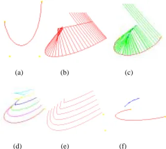
(6) In the previous question, we find the MAT curve goes too far, we will do backtracking. For each backtracking, we do the coordinate transformation and find all the intersection point by the rotated normal vectors of the point in the list and the XY-plane. In the process, we may find the Y-axis intersect two or more bilinear surface generated by consequence rotated normal of boundary points. If the minimum two points whose z-value is near (say its distance less than or equal to a epsilon value)(shown in Figure 6(a)(b)), the branch points can be bounded by the intersection of three bilinear surface, one bilinear is bounded by RN(pi),RN(pi+1), another bilinear surface is bounded by RN(pj),RN(pj+1). The third bilinear surface may be bounded by RN(p1), RN(p2) or RN(p2), RN(p3), assume the current boundary point we are working with is p2. pj. Y. with offset curves, medial axis transform and blending in this section by the examples shown below. Using a Bezier curve generated by the control points (-2.0, 1.0, 0.0),(-1.5, -2.5, 0.0),(1.5, -2.5, 0.0) and (2.0, 3.0, 0.0) as the oriented curve α we consider(shown in Figure 7a), we produce its cyclographic map (Figure 7b), trimmed cyclographic map (Figure 7c), and left local offsets Offl(α,r) (Figure 7d); left global offsets Offg(α,r) (Figure 7e); left medial axis transform MAT+(α)(Figure 7f).. RN(p). pj+1. rj+1. ri+1 ε rj. ri. pi+1. (a). (b). (d). (e). (c). pi. X. p1. p2. (a). (b). Figure 6 Extract the branch from the intersection of three bilinear surface (f). 5. How to terminate at the end point (step 8)? We may check whether the list of points are marked or not. If all of the boundary points in the subdomain are marked, then we are probably near the end point. We may chcek the distances between the unmark point and its two neighbers, if the distance is less than ε, then we quit the process by connect the unmark points with the final MAT point. Otherwise, we insert more boundary between the unmark point and its two neighbors, and continue to march along the MAT curve. We have implemented the algorithms in PC using Visual C++ and OpenGl on Windows 98 and Windows NT. There are about 1,000 lines for the coding of GUI and another 1,000 lines for the ideas of the algorithms.. Figure 7 (a) The oriented curve (b) The cyclographic map (c) The trimmed cyclographic map (d) left local r-offset curves (e) left global r-offset curves (f) left MAT In the omean time, we give the weight function as ω(t)=(1 o t)* 30 +t*60 , where ω(t) is the angle between the rotated normal and the z=0 plane, and produce the weighted cyclographic map (Figure 8a) and trimmed weighted cyclographic map (Figure 8b), local weighted r-offset curve ( Figure 8c), global weighted r-offset curve (Figure 8d) and weighted medial axis transform (Figure 8e).. 4. Application of the Cyclographic Maps We introduce the applications of the Cyclographic Maps in this section. We introduce its relationship with offset curve and with MAT in the first subsection. In the second subsection, we modify the algorithm a little bit on the convex and concave vertices, so that the algorithm extend to handle the curve with singular points. The example for the boundary curve which is closed curve with hole is shown in the third subsection. The fourth subsection introduce the idea that convert the MAT curve back to the origin boundary curve. The final subsection introduce the way we can use cyclographic maps to do corner blending on singular points of curves. 4.1 The relationship between cyclographics and offsets, MAT, and blending curve. We summerize the relationship between cyclographic maps. (a). (b). (d). (c). (e). Figure 8 (a) The weighted cyclographic maps (b) the trimmed weighted cyclographic maps (c) left weighted local r-offset curves (d) left weighted global r-offset curves (e) left weighted medial axis transform 6.

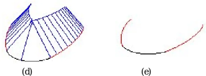
(7) 4.2 Cyclographic Maps at the concave/convex vertex The cyclographic maps at the concave/convex vertex can be trivially produced. We can produce partial cone whose apex is on the convex/concave vertex from the left rotated normal to the right rotated normal. It is a little complex for the weighted cyclographic maps. We have to blend the normal from left rotated normal to the right rotated normal, which means we have to produce a smooth “cone-like” surface to connect two surface produce by two curve to and from the vertex. There are various ways to do the blending, and we select the simply one. That is, we try to do the linear interpolation with the weighted function between the left rotated normal and the right rotated normal. The cyclographic map for convex vertex can be observed from Figure 8 to Figure 9, start from the plane z=r to z=r′, where r′>r and r is the radius of the osculating circle in the point which has local maximal curvature [23]. The cyclograhpic map for the concave vertex is shown in Figure 9 (a) to (e). This concave vertex is the intersection point of two curve generated by two Bezier Curve with control points at (-3.5, -3.0, 0.0),( -3.0, -2.0, 0.0),( -2.0, 0.0, 0.0),( -1.0, 0.5, 0.0) and (-1.0, 0.5, 0.0),( 0.0, 0.0, 0.0),( 1.0, -2.0, 0.0),( 1.5, -3.0, 0.0) respectively. For the weighted cyclographic map, the weighted function for the first and second curves are o o o o ω(t)=(1 - t)* 30 +t*40 and ω(t)=(1 - t)* 50 +t*70 respectively. The (weighted) cyclographic map, (weighted) local offset curve and (weighted) global offset curve, (weighted) medial axis transform are displayed.. (a). (b). (d). (c). (e). Figure 9 (a) The concave vertex of an oriented curve (b) Concave vertex in Cyclographic map (c) local (global) offset (d) concave vertex in Weighted cyclographic maps (e) weighted local (global) offset in the concave vertex.. 4.3 Cyclograhpic Maps for closed simple curve Consider the cyclographic maps for the closed simple curve. The left side of the closed simple curve is bounded, so the medial axis transform is connected with or without loops[28]. But the weighted medial axis transform for closed region is not necessary connected without loop. We may use the same algorithm we mentioned before for weighted medial axis transform, the only difference is the part we calculated at the rotated normal of the boundary. points. The output cyclographic maps for a domain with loop is displayed in Figure 10.. Figure 10 The cyclographic map for a closed domain with loop (a) boundary curve with MAT (b) Cyclographic Map. 4.4 From MAT Curves to its original closed boundary curve As mention in the first section, the footpoint of the MAT point may be found from its MAT curve. We may find all of the boundary points via the MAT curve and generated the original closed boundary curve. We use a queue and a stack to store two parts of the boundary curves. Notice that for the end point on the MAT curve, we have to produce the (weighted) partial cone to connect two boundary points, after connect the boundary points, a list of points has to pop from the stack so that the boundary points are in order. The weighted partial cone is produced by linear interpolation by the angle of the cone, and angle between the line connect the MA point to its two boundary points. 4.5 Blending at the vertex The blending at the concave/convex vertex fix radius blending is produced by truncating the medial axis transform in the cyclographic map below z=r plane, and generated the region of the truncated medial axis transform (as Figure 11) The input boundary curve is generated by two Bezier curves whose control points are (-1.5,1.0,0.0), (-1.5,0.5,0.0),(-1.0,-1.5,0.0), (0.0,-2.0,0.0) and (0.0,-2.0,0.0), (1.0,-1.5,0.0), (1.5,0.5,0.0), (1.5,1.0,0.0) respectively. Notice that in this process, we generated a cone for the end points (cut by z=r plane), so that when we generate the region for the truncated medial axis transform, the corner is smooth. The blending at the concave vertex is similar. Notice that process is only work on vertices. It is not work for the case that z=r cut the medial axis transform in the cyclographic map at a branch without any end point. The various radius blending is produced by truncating the weighted medial axis transform in the weighted cyclographic map below z=r plane, and generated the region of the truncated medial axis transform (as Figure 12). The control points for the boundary curve is the same as the on in Figure 11, except the weighted function for the first curve is o o ω(t)=(1 - t)*45 +t*50 and for the second curve is ω(t)=(1 o o t)* 55 +t*60 .. (a). (b). (c) 7.

(8) 15] 16] (d). (e). Figure 11 The blending at the convex vertex(a) Original curve (b) cyclographic map (c) cut by z=r (d) produce the cone (e) back to z=0 plane. 17]. 18]. 19] (a) Original curve (b) blending at the vertex Figure 12 The varius radius blending 20] 5. REFERENCES 1] Bruce and Giblin, “Curve and Surface”. 2] R. T. Farouki and C. A. Neff. Analytic properties of plane offset curves. Computer Aided Geometric Design, 7:83--100, 1990. 3] C. M. Hoffmann. Geometric and Solid Modeling. Morgan Kaufmann, San Mateo, Cal., 1989. 4] J. Hoschek. Grundlagen der Geometrischen Datenverarbeitung. Teubner Verlag, Stuttgart, 1989. 5] H. Blum. A transformation for extracting new descriptors of shape. In W. Whaten-Dunn, editor, Models for the Perception of Speech and Visual Form}, pages 362--380. MIT Press, Cambridge, MA, 1967. 6] Christoph M. Hoffmann. Computer vision, descriptive geometry and classical mechanics. In B. Falcidieno and I. Hermann, editors, Computer Graphics and Mathematics. Springer Verlag, 1992. 7] Harry Blum, Biological Shape and Visual Science (Part I), Journal Theoretical Biology, 38:205-287, 1973. 8] Azriel Rosenfeld and John L. Pfaltz, Sequential Operations in digital Picture Processing,Journal of ACM, 13(4):471-491, 1966. 9] John L. Pfaltz and Azriel Rosenfeld, Computer Representation of Planar Regions by Their Skeleton, Communications of the ACM, 10(2):119-125,1967. 10] C. Judith Hilditch, Linear Skeletons from Square Cupboards, Machine Intelligence, 3:325-420, 1968. 11] Otis Philbrick, Shape Description with the Medial Axis Transformation, Pictorial Pattern Recognition, pages 395-407, Thompson Book Co. 1968. 12] Harry Blum and Roger N. Nagel, Shape Descriptiion Using Weighted Symmetric Axis Features, Pattern Recognition, 10:167-180, 1978. 13] Halit Nebi Gursoy,Shape Interrogation by Medial Axis Transform for Automated Analysis, Ph.D. Thesis. 14] N.M.. Patrikalakis and H.N. Gursoy, Shape interrogation by Medial Axis Transform, Technical. 21] 22] 23]. 24]. 25]. 26] 27]. 28]. 29]. 30]. Report, Design Lab. Memo. 90-2, Sea Grant College Program, MIT, 1990. T.K.H Tam and C.G. Armstrong, 2D Finite Element Mesh Generation by Medial Axis Subdivision, 1992. V. Srinivasan, L. Nackman, J. Tang and S. Meshkat, Automatic mesh generation using the symmetric axis transformation of polygonal domains, Technical Report RC 16132, IBM Yorktown Heights, 1990. Sabine Stifter, The Roider method: A method for static and dynamic ollision detection, In C. Hoffmann, editor, Issues in Robotics and Nonlinear Geometry, JAI press, 1990. C.N. Chu, R.L.Kashyap, T.C Lee and I.C. You, Castability Evaluation via keleton-Based Modeling, CIDMAC Annual Report, Schools of Engineering, Purdue University, 1990-1991. Christoph M. Hoffmann and George Vanecek, Jr., Fundamental Techniques for Geometric and Solid Modelling, In C.T. Leondes, editors, Advances in Control and Dynamics. Academic Press, 1991. E. Müller and J. Krames. Die Zyklographie. Franz Deuticke, Leipzig und Wien, 1929. J. Plucker. On a new geometry of space. Phil. Trans R. Soc., 155, 1865. Christoph M. Hoffmann, A dimensionality paradigm for surface interrogations. CAGD, 7:517--532, 1990. Rida T. Farouki and Jean-Claude A. Chastang. Evolving wavefronts as algebraic curves, Technical Report Technical Report RC-16381, IBM Yorktown Heights, 1990. R. T. Farouki, The approximation of nondegenerate offset surfaces, Computer Aided Geometric Design, 3:15--43, 1986. R. T. Farouki and C. A. Neff., Algebraic properties of plane offset curves. Computer Aided Geometric Design, 7:101--128, 1990. J. Hoschek, Offset curves in the plane, Computer Aided Design, 17:77--82, 1985. J. Hoschek and N. Wissel, Optimal approximate conversion of spline curves and spline approximation of offset curves. Computer Aided Design, 20:475--483, 1988. Ching-Shoei Chiang, The Euclidean Distance Transform, Ph.D. Thesis, Department of Computer Science, August, 1992. Hyeong In Choi, Sung Woo Choi, Hwan Pyo Moon and Nam Sook Wee, New Algorithm for Medial Axis Transform of Plane Domain, Technique Report RIM-GARC Preprint Series 95-88, Department of Mathematics, Seoul National University. Hyeong In Choi, Sung Woo Choi and Hwan Pyo Moon, Mathematical Theory of Medial Axis Transform, Technique Report RIM-GARC Preprint Series 95-87, Department of Mathematics, Seoul National University.. 8.

(9)