Using Threshold Error-Correction Model to Investigate Asymmetric Price Transmissions between the Real Estate and Stock Markets in Taiwan

全文

(1)Using Threshold Error-Correction Model to Investigate Asymmetric Price Transmissions between the Real Estate and Stock Markets in Taiwan. Tsangyao Chang* Department and Graduate Institute of Economics Feng Chia University, Taichung, TAIWAN Chien-Chung Nieh Department of Banking & Finance Tamkang University, Taipei, TAiWAN. ABSTRACT In this study, using a threshold error-correction model, we investigate price transmissions between the real estate and stock markets in Taiwan over the 1986Q1 to 2003Q2 period. The results from Granger-Causality tests based on corresponding threshold error-correction model (TECM) clearly point to unidirectional causality running from the real estate market to stock market in the short run. Furthermore, we find asymmetric price transmissions between these two markets in the long run. These findings ought to be made readily available to individual investors and financial institutions holding long-term investment portfolios in these two asset markets for their likely implications today. JEL: C32; G11 Key Words: Threshold Error-Correction Model, Real Estate and Stock Markets, Asymmetric Price Transmissions. ____________ *Corresponding author: Professor, Department and Graduate Institute of Economics, Feng Chia University, Taichung, Taiwan. TEL: 4- 2451-7250 ext. 4484. FAX: 4-2451-8737. E-mail: tychang@fcu.edu.tw. 1 第五屆全國實證經濟學論文研討會 The 5th Annual Conference of Taiwan's Economic Empirics.

(2) I. INTRODUCTION Identifying the relationship between real estate prices and stock prices has been a widely debated issue within academic circles and among practitioners, alike. Although current literature on the relationship between real estate and equity markets tends to show conflicting results, most of the empirical evidence seems to support the view that the two markets are segmented.. Goodman (1981), Miles et al., (1990), Liu. et al., (1990) and Geltner (1990), for example, argue for the existence of such segmentation within various real estate markets and stock markets.. In direct contrast,. Liu and Mei (1992), Ambrose et al. (1992) along with Gyourko and Keim (1992), report results that contradict that position, claiming that real estate and stock markets are in fact integrated.. The predicament faced here, therefore, is whether the two. markets are segmented or integrated.. Our primary objective then is to ascertain. whether any significant relationship does exist between these markets and, if so, to determine what implications it may have for active market traders.. One fundamental. motivation behind our study is that our findings can yield considerable insight for both investors and speculators that may facilitate forecasting future performance from one market to the other. While previous studies focus on linear relationship between these two markets with the exception of Okunew and Wilson (1997), in this study, using a recently developed threshold error-correction model advanced by Enders and Granger (1998) and Enders and Siklos (2001), we investigate price transmissions between the real estate and stock markets in Taiwan over the 1986Q1 to 2003Q2 period. The results from Granger-Causality tests based on corresponding threshold error-correction model (TECM) clearly point to unidirectional causality running from the real estate market to stock market. Further, asymmetric price transmissions between these two markets are also found in the long run. The remainder of this study is organized as follows. data used.. Section II presents the. Section III presents the methodologies used and discusses the findings.. Finally, Section IV concludes.. II. DATA The data sets used here consist of quarterly time series on the real estate price index (lresp) and stock price index (lstkp) for the 1986Q1 to 2003Q2 period. 2 第五屆全國實證經濟學論文研討會 The 5th Annual Conference of Taiwan's Economic Empirics. The stock.

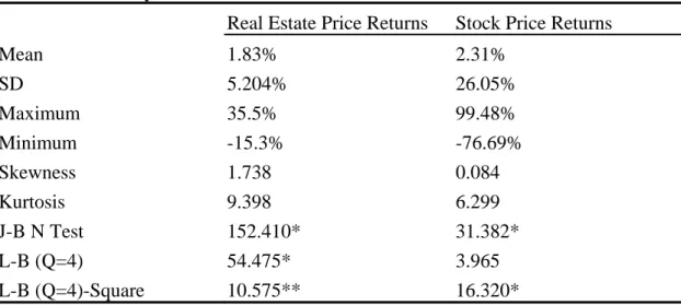
(3) price indexes are obtained from the AREMOS database of the Ministry of Education of Taiwan.. The real estate price index is collected and compiled by Hsin-Yi Real. Estate Inc.. An examination of the individual data series makes it clear that. logarithmic transformations are required to achieve stationarity in variance; therefore, all the data series are transformed to logarithmic form. Descriptive statistics for both real estate and stock markets returns are reported in Table 1.. We find that the sample means of the real estate price returns are. positive (1.83%) and the stock price returns are also positive (2.31%).. Both the. skewness and kurtosis statistics indicate that the distributions of the returns of both markets are non-normal.. The Ljung-Box statistics for 4 lags applied to the returns. and square returns indicate that significant linear and non-linear dependencies exist in the real estate market.. However, we only find significant non-linear dependencies in. the stock market. 「Insert Table 1 Here」. III METHODOLOGY AND EMPIRICAL RESULTS A. Unit Root Tests Recently, there is a growing consensus that stock price and real estate price might exhibit nonlinearities and that a conventional test such as the ADF unit root test has lower power in detecting its mean reverting tendency.. The finding of nonlinear. adjustment does not necessary imply nonlinear mean reversion (stationary).. As such,. formal stationary tests based on nonlinear framework much be applied.. In this. study, our major objective is to determine whether the stock price and real estate price are nonlinear stationary, based on a nonlinear stationary test advanced by Kapetanios et al. (2003) (henceforth, KSS test) Since it is a brand new test, we will briefly describe this test in the following. According to Kapetanois et al. (2003), their test is based on detecting the presence of non-stationarity against nonlinear but globally stationary exponential smooth transition autoregressive (ESTAR) process:. ∆Yt = γYt −1{1 − exp(−θYt −21 )} + ν t ,. [1]. where Yt is the data series of interest, vt is an i.i.d. error with zero mean and constant variance and θ ≥ 0 is known as the transition parameter of the ESTAR model that governs the speed of transition. We are now interested in testing the null hypothesis 3 第五屆全國實證經濟學論文研討會 The 5th Annual Conference of Taiwan's Economic Empirics.

(4) of θ = 0 against the alternative θ > 0 . Under the null Yt follows a linear unit root process, whereas it is nonlinear stationary ESTAR process under the alternative. However, the parameter γ is not identified under the null hypothesis. Following Luukkonen et al. (1988) and Kapetanios et al. (2003), we use a first-order Taylor series approximation to { 1 − exp(−θYt 2−1 ) } under the null θ = 0 and approximate. Equation [1] by the following auxiliary regression: k. ∆Yt = ξ + δYt 3−1 + ∑ bi ∆Yt −i +ν t , t = 1, 2,…., T. [2]. i =1. Then, the null hypothesis and alternative hypotheses are expressed as δ = 0 (nonstationarity) against. δ < 0 (non-linear ESTAR stationarity). The simulated critical values for different K are tabulated at Kapetanios et al.’s (2003) Table 1 of their paper. Table 2 reports the Kapetanios et al. (2003) nonlinear stationary test results indicating that both two series are integrated of order one. For comparison, we also incorporate the PP, NP (Ng and Perron, 2001) and KPSS (Kwiatkowski et al., 1992) tests into our study. Panels A and B in Table 3 present the results of the non-stationary tests for the stock price index (lstkp) and real estate price index (lresp) from the PP, NP and KPSS tests. We find each data series is nonstationary in levels but stationary in first differences, suggesting that all the data series are integrated of order one. On the basis of these results, we proceed to test whether these two variables are cointegrated, and to do so, we used the recently developed threshold cointegration tests. 「Insert Tables 2 and 3 Here」. B. Threshold Cointegration Tests Based on Enders and Granger (1998) and Enders and Siklos’s (2001) Approach The Enders-Granger’s threshold cointegration test consists of a two-stage procedure. Following Enders and Granger (1998) and Enders and Siklos (2001), in the first stage, we estimate the cointegration equations as follows: Y1t = α + βY2t + u t. [3]. where Y1t and Y2t are stock price index and real estate price index, respectively, and both are integrated of order 1 or I(1).. α and β are estimated parameters, and u t 4. 第五屆全國實證經濟學論文研討會 The 5th Annual Conference of Taiwan's Economic Empirics.

(5) is the disturbance term that may be serially correlated. The second stag focuses on the OLS estimates of ρ1 and ρ 2 in the following regression: l. ∆u t = I t ρ1u t −1 + (1 − I t ) ρ 2 u t −1 + ∑ γ i ∆u t −i + ε t. [4]. i =1. where ε t is a white-noise disturbance and the residuals( µ t ) from [3] are used to estimate [4].. I t is the Heaviside indicator function such that I t = 1 if u t −1 ≥ τ ,. I t = 0 if u t −1 ≤ τ and τ = the value of threshold. A necessary condition for { µ t } to be stationary is: − 2 < ( ρ1 , ρ 2 ) < 0 . If the variance of ε t is sufficiently large, it is also possible for one value of ρ j to between –2 and 0 and for the other value to equal zero. Although there is no convergence in the regime with the unit-root (i.e., the regime in which ρ j = 0 ), large realization of ε t will switch the system into the convergent regime.. Enders and Granger (1998) and Enders and Siklos (2001) both. point out in either case, under the null hypothesis of no convergence, the F-statistic for the null hypothesis ρ1 = ρ 2 = 0 has a nonstandard distribution. The critical values for this non-standard F-statistic are tabulated in their paper.. Enders and. Granger (1998) also show that if the sequence is stationary, the least squares estimates of ρ1 and ρ 2 have an asymptotic multivariate normal distribution. Model using [4] is referred to as Threshold Autoregression Model (TAR), where the test for threshold behavior of the equilibrium error is termed threshold cointegration test.. Assuming the system is convergent, µ t = 0 can be considered. as the long-run equilibrium value of the sequence. If µ t is above its long-run equilibrium, the adjustment is ρ1 µ t −1 and if µ t is below its long-run equilibrium, the adjustment is ρ 2 µ t −1 . autoregression.. The equilibrium error therefore behaves like a threshold. Thus, if the null hypothesis ρ1 = ρ 2 = 0 is rejected, it is possible. to test for symmetric adjustment (i.e., ρ1 = ρ 2 ) using a standard F-test.. Since. adjustment is symmetric if ρ1 = ρ 2 , the Dickey-Fuller test is a special case of [4]. Rejecting both the null hypothesis of ρ1 = ρ 2 = 0 and ρ1 = ρ 2 imply that the residuals in [3] are stationary and the existence of threshold cointegraiton. Instead of estimating [4] with the Heaviside indicator depending on the level of. µ t −1 , the decay could also be allowed to depend on the previous period’s change 5 第五屆全國實證經濟學論文研討會 The 5th Annual Conference of Taiwan's Economic Empirics.

(6) in µ t −1 .. The Heaviside indicator could then be specified as I t = 1 if ∆u t −1 ≥ τ ,. I t = 0 if ∆u t −1 ≤ τ and τ = the value of threshold.. According to Enders and. Granger (1998), this model is especially valuable when adjustment is asymmetric such that the series exhibits more ‘momentum’ in one direction than the other.. This. model is termed Momentum-Threshold Autoregression Model (M-TAR). The TAR model can capture ‘deep’ cycle process if, for example, positive deviations are more prolonged than negative deviations.. The M-TAR model allows the autoregressive. decay to depend on ∆µ t −1 . As such, the M-TAR representation can capture ‘sharp’ movements in a sequence. In the most general case, the value of τ is unknown, it needs to be estimated along with the value of ρ1 and ρ 2 . By demeaning the { µ t } sequence, the Enders and Granger (1998) test procedure actually employs the sample mean of the sequence as the threshold estimate of τ .. Nevertheless, the sample mean is a biased threshold. estimator in the presence of asymmetric adjustments.. For instance, if autoregressive. decay is more sluggish for positive deviations of µ t −1 from τ than for negative deviations, the sample mean estimator will be biased upwards.. A consistent estimate. of the threshold τ can be obtained by using Chan’s (1993) method of searching over possible threshold values to minimize the residual sum of squares form the fitted model. Enders and Siklos (2001) apply Chan’s methodology to a Monte Carlo study to obtain the F-statistic for the null hypothesis for ρ1 = ρ 2 = 0 when the threshold. τ is estimated using Chan’s procedure.. The critical values of this non-standard. F-statistic for testing the null hypothesis of ρ1 = ρ 2 = 0 are also tabulated in their paper. As there is generally no presumption as to whether to use TAR or M-TAR model, the recommendation is to select the adjustment mechanism by a model selection criterion such as the AIC or SBC. Table 4 reports the threshold cointegration test results. From the AIC and SBC, we find the most preferable model for our adjustment mechanism is TAR model (where the threshold value of τ = 0.32103 is also found based on the Chan’s (1993) method).. Since the null of no cointegration ( ρ1 = ρ 2 = 0 ) and symmetric. adjustment ( ρ1 = ρ 2 ) are both rejected, these imply the existence of threshold cointegraiton between the real estate and stock markets in Taiwan over this testing. 6 第五屆全國實證經濟學論文研討會 The 5th Annual Conference of Taiwan's Economic Empirics.

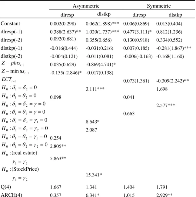
(7) period. 「Insert Table 4 Here」. C. Granger-Causality Tests Based on Threshold Error-Correction Model Given the threshold cointegration found in previous section, we proceed to test the price transmissions using threshold error-correction model (TECM).. The TECM. can be expressed as follows (Enders and Granger, 1998; Enders and Siklos, 2001): k1. k2. i =1. i =1. ∆Yit = γ 1 Z − plus t −1 + γ 2 Z − min us t −1 + ∑ θ i ∆Y1t −i + ∑ δ i ∆Y2t −i +vt. [5]. where Yit = (lrespt , lstkpt ) , Z − plus t −1 = I t uˆ t −1 , Z − min ust −1 = (1 − I t )uˆ t −1 such that I t = 1 if u t −1 ≥ 0.32103 , I t = 0 if u t −1 ≤ 0.32103 and vt is a white-noise disturbance.. From the system, the Granger-Causality tests are examined by testing. whether all the coefficients of ∆Y1,t −i or ∆Y2,t −i are statistically different from zero as a group based on a standard F-test and/or whether the ρ j coefficient of the error-correction are also significant.. Since Granger-Causality tests are very sensitive. to the selection of lag length, the lag lengths are determined using Hsiao’s (1979) sequential procedures, which are based on the Granger definition of causality. Based on this procedure, we find both lags length of k1 = k 2 = 2 . Table 5 presents the results from our Granger-Causality tests based on the corresponding threshold error-correction models (TECMs).. They clearly show that. unidirectional causality running from the real estate market to the stock market in the short-run.. This result is consistent with those found in Liu and Mei (1992),. Ambrose et al. (1992) along with Gyourko and Keim (1992).. In terms of long-run. situation, however, we find feedback exists between these two markets.. The. empirical results show unidirectional causality running from the real estate market to stock market when the threshold variable is above 0.32103. On the other hand, when the threshold variable is below 0.32103, we find unidirectional causality running from the stock market to real estate market.. These empirical results indicate. that the price transmissions between these two markets are asymmetric in the long run. It is interesting to note that the adjustment coefficients of Z − plus and Z − min us are markedly different for both markets. Focusing on adjustments of real estate market to restore equilibrium, the point estimates of adjustment coefficients given in 7 第五屆全國實證經濟學論文研討會 The 5th Annual Conference of Taiwan's Economic Empirics.

(8) Table 5 indicate that, within a quarter, real estate prices adjust so as to eliminate approximately 13.5% of a unit negative change in the deviation from the equilibrium relationship created by changes in stock prices.. On the other hand, real estate prices. adjust by only 3.5% of a positive change in deviation from the equilibrium created by changes in stock prices.. These findings indicate that adjustments towards the. long-run equilibrium relationship between the real estate and stock markets are faster when changes in deviation are negative than when they are positive. stock market, we find the reverse adjustment process.. In terms of. Within a quarter, stock prices. adjust so as to eliminate approximately 1.7% (86.9%) of a unit negative (positive) change in the deviation from the equilibrium relationship created by changes in real estate prices. These findings indicate that adjustments towards the long-run equilibrium relationship between the real estate and stock markets are faster when changes in deviation are positive than when they are negative. Indeed, F-statistic also indicates that the null hypotheses of γ 1 = γ 2 (the coefficients of Z − plus and Z − min us are equal) from both markets are rejected.. Further, we find that the. error-correction term is significant for the equation concerning for stock market when the threshold variable is above 0.32103, however when the threshold variable is below 0.32103, the error-correction term is significant for the equation concerning for real estate market.. Our interpretation is that, over time, as measured by the. error-correction term, in order to restore the long-run relationship within system, it is real estate (stock) prices that must bear the brunt of adjustment rather than stock (real estate) prices, when the threshold variable is below (above) the value of 0.32103. These empirical results further indicate that price transmissions between these two markets are asymmetric. By way of contrast, Table 5 also reports the estimates of symmetric error-correction model.. In the case of symmetric adjustment, only the. error-correction term on the stock market is significant at conventional levels. This result implies that the stock prices but not the real estate prices bear the brunt of adjustment process.. In spite of the extra coefficient appearing in each equation of. threshold model, the multivariate AIC selects threshold error-correction model over the symmetric error-correction model.. The multivariate AIC is 70.151 for the. threshold error-correction model and 81.295 for the symmetric error-correction model. 8 第五屆全國實證經濟學論文研討會 The 5th Annual Conference of Taiwan's Economic Empirics.

(9) 「Insert Table 5 Here」. IV. CONCLUSIONS In this study we investigate the relationship between the real estate and stock markets in the Taiwan context over the 1986Q1 to 2003Q2 period, using a recently developed threshold error-correction (TECM). Granger-Causality test results from the corresponding TECM clearly point to unidirectional causality running from the real estate market to stock market in the short run.. Furthermore, we find asymmetric. price transmissions between these two markets in the long run.. In terms of risk. diversification, the two assets should not have been included in the same portfolio in Taiwan during the 1986Q1 to 2003Q2 period. Consequently, these findings ought to be made readily available to individual investors and financial institutions holding long-term investment portfolios in these two asset markets for their likely implications today.. 9 第五屆全國實證經濟學論文研討會 The 5th Annual Conference of Taiwan's Economic Empirics.

(10) REFERENCES. Ambrose. B., Ancel, E. and Griffiths, M., (1992) “The Fractual Structure of Real Estate Investment Trust Returns: A Search for Evidence of Market Segmentation and Nonlinear Dependency”, Journal of the American Real Estate and Urban Economics Association, 20(1), pp25-54. Campbell, J and Perron, Peter., What Macroeconomists Should Know about Unit Roots, edited by O. Blanchard and S. Fish, NBER Macroeconomics Annual, MIT Press, Cambridge, MA. 1991. Chan, K.S. (1993) “Consistency and Limiting Distribution of the Least Squares Estimator of a Threshold Autoregressive Model”, The Annals of Statistics, 21, pp520-533. Dickey, David A., Bell, W. R., and Miller, R. B., (1986) “Unit Root in Time Series Models: Tests and Implications”, The American Statistician, 40, 1, 12-26. Enders, W., and Granger, C.W. F. (1998) “Unit-root tests and asymmetric adjustment with an example using the term structure of interest rates”, Journal of Business Economics & Statistics, 16, pp304-311. Enders, W. and Siklos, P.L., (2001) “Cointegration and Threshold Adjustmetn”, Journal of Business Economics & Statistics, 19, pp166-176. Engle, Robert and Granger, C. W. J., (1987) “Cointegration and Error Correction: Representation, Estimation, and Testing”, Econometrica, 55, 251-276. Geltner, D., (1990) “Return Risk and Cash Flow with Long Term Riskless Leases in Commercial Real Estate”, Journal of the American Real Estate and Urban Economics Association, 18, pp377-402. Goodman, A.C., (1981) “Housing Submarkets Within Urban Area: Definitions and Evidence”, Journal of Regional Science, 21(2), pp175-185. Gyourko, J and Keim, D., (1992) “What Does the Stock Market Tell Us About Real Returns”, Journal of the American Real Estate Finance and Urban Economics Association, 1992, 20(3), pp457-486. Hsiao, Cheng. (1979) Causality in econometrics, Journal of Economic Dynamics and Control, 4, 321-346. Kapetanios, G., Shin Yongcheol., and Snell, A. (2003) “Testing for a unit root in the nonlinear STAR framework”, Journal of Econometrics, 112, pp359-379. Kwiatkowski, Denis, Phillips, Peter, Schmidt, Peter and Shin, Yongcheol., (1992) “Testing the Null Hypothesis of Stationarity Against the Alternative of A Unit Root: How Sure Are We That Economic Time Series Have A Unit Root ?” Journal of Econometrics, 54, 159-178. Liu, C. and Mei, J., (1992) “The Predictability of Returns on Equity REIT’s and Their 10 第五屆全國實證經濟學論文研討會 The 5th Annual Conference of Taiwan's Economic Empirics.

(11) Co-movements With Other Assets”, Journal of Real Estate Finance and Economics, 5, pp401-418. Liu, C., Hartzell, D., Greig, D.W., and Grissom, T.V., (1990) “The Integration of The Real Estate Market and The Stock Market: Some Preliminary Evidence”, Journal of Real Estate Finance and Economics, 3, pp261-282. Luukkonen, R., Saikkonen, P., Terasvirta, T. (1988) “Testing Linearity against smooth transition autoregressive models”, Biometrika, 75, pp491-499. Mackinnon, James., Critical Values for Cointegration Tests in Long-Run Economic Relationships - Readings in Cointegration, edited by Engle and Granger, Oxford University Press.1991. Miles, M. Cole, R and Guikey., (1990) “A Different Look At Commercial Real Estate Returns”, Journal of the American Real Estate and Urban Economics Association, 18(4), pp403-430.. Newey, Whitney and West, Kenneth. (1994) “Automatic Lag Selection in Covariance Matrix Estimation”, Review of Economic Studies, 61, pp631-653. Ng, Serena., and Perron, Pierre. (2001) “Lag Length Selection and the Construction of Unit Root Tests with Good Size and Power”, Econometrica, 69, pp1519-1554. Okunew, J. and Wilson, P J., (1997) “Using Nonlinear Tests to Examine Integration Between Real Estate and Stock Markets”, Real Estate Economics, 25, 3, 487-503. Perron, P., (1989) “The Great Crash, The Oil Price Shock and The Unit Root Hhypothesis”, Econometrica, 57(6), 1361-1401. Perron, P., (1990) “Testing for A Unit Root in A Time Series with A Changing Mean”, Journal of Business Economics and Statistics, 8, 2, 153-162. Zivot, E., and Andrews, D.W.K., (1992) “Further Evidence on The Great Crash, The Oil Price Shock, and The Unit Root Hypothesis”, Journal of Business and Economic Statistics, 10, 251-270.. 11 第五屆全國實證經濟學論文研討會 The 5th Annual Conference of Taiwan's Economic Empirics.

(12) Table 1. Summary Statistics of Real Estate and Stock Markets Returns. Mean SD Maximum Minimum Skewness Kurtosis J-B N Test L-B (Q=4) L-B (Q=4)-Square. Real Estate Price Returns. Stock Price Returns. 1.83% 5.204% 35.5% -15.3% 1.738 9.398 152.410* 54.475* 10.575**. 2.31% 26.05% 99.48% -76.69% 0.084 6.299 31.382* 3.965 16.320*. Note: 1. SD denotes standard error. 2. The standard errors of the skewness and kurtosis are (6 / T ) 0.5 and (24 / T ) 0.5 , respectively. J-B N Test denotes the Jarque-Bera normality test. 4. L-B (Q=k) represents the Ljung-Box test for autocorrelation up to k lags. 5. *, ** and *** indicate significance at the 1%, 5% and 10%, respectively. 3.. Table 2. Unit Root Test based on KSS (2003) Approach. t Statistic on δˆ lresp lstkp. 0.308(1) -0.094(0). Note: The numbers in the parentheses are the appropriate lag lengths selected by MAIC (modified Akaike information criterion) suggested by Ng and Perron (2001).. Table 3. PP , NP and KPSS Unit Root Tests. Panel A: PP level. difference. Panel B: KPSS ( η µ ). Panel A: NP level. difference. level. difference. 0.126(6)** *. 0.074(6). -2.657(2)** 0.215(6)** *. 0.051(5). Lresp. -2.531(4) –5.051(3)* -2.922 (0) -9.517(0)*. Lstkp. –2.819(4) –9.605(3)* -1.932 (3). Note: 1. The number in the parentheses of NP are the appropriate lag lengths selected by MAIC (modified Akaike information criterion) suggested by Ng and Perron (2001), whereas the number in the parentheses of PP and KPSS are the optimal bandwidth decided by Bartlett kernel of Newey and West (1994). 2. *, **, and *** denote significance at the 1%, 5% , and 10% levels, respectively. 3. Critical values for the KPSS test are taken from Kwiatkowski et al. (1992). 4. The test statistic for NP is MZ t .. Table 4. Threshold Cointegration Tests Based on the Enders and Granger (1998) Approach (TAR model where the threshold value of τ = 0.32103 ) ρˆ 1 ρˆ 2 FˆC Fˆ A l. -0.646(5.109)*. -0.066(0.095). 13.296*. 13.429*. 0. Note: 1. *, **, and *** denote significance at the 1%, 5% , and 10% levels, respectively. Lag-length ( l ) selection is based on the procedure advanced by Perron (1989). 2. t statistics are in parentheses. FˆC and Fˆ A denote the F-statistics for the null hypothesis of 12 第五屆全國實證經濟學論文研討會 The 5th Annual Conference of Taiwan's Economic Empirics.

(13) no cointegraion and symmetry.. Critical values are taken from Enders and Siklos (2001). Table 5. Estimates of the Error-Correction Models. Asymmetric dlstkp dlresp Constant dlresp(-1) dlresp(-2) dlstkp(-1) dlstkp(-2) Z − plus t −1 Z − min ust −1 ECTt −1 H 0 : δ1 = δ 2 = 0 H 0 : θ1 = θ 2 = 0 H 0 : δ1 = δ 2 = γ = 0 H 0 : θ1 = θ 2 = γ = 0 H 0 : δ1 = δ 2 = γ 1 = 0 H 0 : δ1 = δ 2 = γ 2 = 0 H 0 : θ1 = θ 2 = γ 1 = 0 H 0 : θ1 = θ 2 = γ 2 = 0. 0.002(0.298). Symmetric dlresp. 0.062(1.898)*** 0.006(0.869). dlstkp 0.013(0.404). 0.388(2.637)** 1.020(1.737)*** 0.477(3.111)* 0.812(1.236) 0.092(0.681) 0.355(0.656) 0.130(0.918) 0.334(0.552) -0.016(0.444). -0.031(0.216). 0.007(0.185). -0.281(1.867)***. -0.004(0.121). -0.011(0.081). -0.006(-0.163) -0.168(1.160). 0.035(0.629). -0.869(4.741)*. -0.135(-2.846)* -0.017(0.138) 0.073(1.361) 3.111***. -0.309(2.242)** 1.698. 0.098. 0.041 2.577*** 0.663 8.643* 2.087. 0.254 2.805**. H 0 : (real estate). γ1 = γ 2. 5.863**. H 0 : (StockPrice) 15.341*. γ1 = γ 2 Q(4) ARCH(4). 1.667. 1.341. 1.404. 1.791. 0.357. 6.341*. 1.015. 2.929**. Note: 1. *, **, and *** denote significance at the 1%, 5% , and 10% levels, respectively. are in parentheses. 2. Threshold Error-Correction Model: k1. k2. i =1. i =1. t statistics. ∆Yit = γ 1 Z − plust −1 + γ 2 Z − min ust −1 + ∑ θ i ∆Y1t −i + ∑ δ i ∆Y2t −i +vt where Yit = (lrespt , lstkpt ) , Z − plus t −1 = I t uˆ t −1 , Z − min us t −1 = (1 − I t )uˆ t −1 such that I t = 1 if u t −1 ≥ 0.32103 , I t = 0 if u t −1 ≤ 0.32103 and vt is a white-noise disturbance. 3. Symmetric Error-Correction Model: ∆Yit = γuˆ t −1 +. k1. k2. i =1. i =1. ∑θ i ∆Y1t −i + ∑ δ i ∆Y2t −i +vt. 13 第五屆全國實證經濟學論文研討會 The 5th Annual Conference of Taiwan's Economic Empirics.

(14)