For Peer Review
A Robust TDT-Type Association Test under Informative Parental Missingness
Journal: Statistics in Medicine Manuscript ID: Draft
Wiley - Manuscript type: Paper Date Submitted by the
Author:
Complete List of Authors: Chen, Jin-Hua; China Medical University, Graduate Institute of Biostatistics
Cheng, K.F.; National Central University, Statistics(Biostatistics Branch); China medical University, Biostatistics Center and Department of Public Health
Keywords: Association test, Case-parents study, Informative missigness, Robustness, Transmission /disequilibrium test
For Peer Review
A Robust TDT-Type Association Test under Informative Parental
Missingness
J.H. Chena and K.F. Chengb,c
a
Biostatistics Center and Graduate Institute of Biostatistics, China Medical University,
Taichung, Taiwan (ROC) b
Biostatistics Center and College of Public Health, China Medical University, Taichung,
Taiwan (ROC) c
Graduate Institute of Statistics, National Central University, Chungli, Taiwan (ROC)
Short Title: Robust TDT-type Association Test
Correspondence to Professor: K.F. Cheng, Biostatistics Center, China Medical University,
Taichung, Taiwan (ROC). E-mail: [email protected].
Phone number: 886-4-2207-8539. Fax: 886-4-22078539.
3 4 5 6 7 8 9 10 11 12 13 14 15 16 17 18 19 20 21 22 23 24 25 26 27 28 29 30 31 32 33 34 35 36 37 38 39 40 41 42 43 44 45 46 47 48 49 50 51 52 53 54 55 56 57 58 59 60
For Peer Review
Many family-based association tests rely on the random transmission of alleles from parents
to offspring. Among them, the transmission/disequilibrium test (TDT) may be considered to
be the most popular statistical test. The TDT statistic and its variations were proposed to
evaluate nonrandom transmission of alleles from parents to the diseased children. However, in
family studies, parental genotypes are not always available. Quite often, the offspring
genotype affects the severity of offspring phenotype or/and the age at onset and in turn affects
the parental missingness. In such case, the nonrandom transmission of alleles may also occur
even when the gene and disease are not associated. As a consequence, the usual TDT-type
tests would produce excessive false positive conclusions in association studies. In this paper,
we propose a TDT-type association test which is not only simple in computation but also
robust to the joint effect of population stratification and informative parental missingness. The
test statistic does not rely on any model and also allows for having different mechanisms of
parental missingness across subpopulations. We use a simulation study to compare the
performance of new test and the TDT and point out the advantage of the new method.
Keywords: Association test; Case-parents study; Informative missigness; Robustness;
Transmission /disequilibrium test
3 4 5 6 7 8 9 10 11 12 13 14 15 16 17 18 19 20 21 22 23 24 25 26 27 28 29 30 31 32 33 34 35 36 37 38 39 40 41 42 43 44 45 46 47 48 49 50 51 52 53 54 55 56 57 58 59 60
For Peer Review
1. Introduction
Testing association between genetic markers and disease usually consists of a comparison of
genotypes from a sample of diseased individuals with those from a certain sample of
nondiseased individuals. The usual case-parents study suggests using genotype data of the
diseased children and their parents for making inference about gene-disease association. Well
known tests based on parental controls include the transmission/disequilibrium test (TDT)
proposed by Spielman et al. [1], and the conditional-on-parental-genotypes (CPG) tests
proposed by Schaid and Sommer [2] (see also [3]-[7]) for related approaches. The TDT and
the CPG tests are identical under additive genetic model. However, the CPG approach is
generally more powerful than the TDT approach under other genetic models.
In case-parents study, the cases and controls are matched in genetic ancestry. Thus, the
analysis based on the TDT or CPG tests is free of bias arising from population stratification.
This is an important property for valid association tests. However, these tests may still
produce biased results if informative parental missingness exists in the study. The effect of
missing parental genotype and its correction were studied by Clayton [8], Sun et al. [9],
Weinberg [10], Cervino and Hill [11], Allen et al. [12], and Chen [13] (see also Robinwitz and
Laird [14]; Robinwitz [15] for tests based on general families.) However, many of these
methods often require assumptions such as missing-at-random (MAR, conditional on
3 4 5 6 7 8 9 10 11 12 13 14 15 16 17 18 19 20 21 22 23 24 25 26 27 28 29 30 31 32 33 34 35 36 37 38 39 40 41 42 43 44 45 46 47 48 49 50 51 52 53 54 55 56 57 58 59 60
For Peer Review
offspring and available parent, the genotype frequencies among missing parents and among
observed parents are the same) or missing-independent-of-offspring-genotype (MIOG,
conditional on parental genotypes, the parental missingness is independent of offspring’s
genotype). Since there is no genotype information available on the missing parents, thus these
important assumptions are usually difficult to justify in real applications. Another assumption
also often required in some association tests is that the response probabilities of parents can be
modeled by the same parametric function across all families in the study sample. For example,
Allen et al. [12] required that the response-odds parameters satisfy relatively simple models
across all studied families. This assumption may not be credible either, if the overall
population consists of several subpopulations and response rates have different forms across
subpopulations.
In the paper, we first point out that when there is no disease-gene association, and both
parents are observed, the probability of offspring’s genotype conditional on the parental
genotypes (general CPG probabilities) are no longer the same as the usual Mendelian
proportions, if the parental missingness also depends on the offspring genotype. In this case,
many tests such as TDT or its variations, depending on using the properties of
Schaid-Sommer’s CPG probability, would produce biased association results. This particular
case may occur when, for example, the offspring genotype affects the severity of offspring
phenotype or/and the age at onset and in turn affects the parental missingness.
3 4 5 6 7 8 9 10 11 12 13 14 15 16 17 18 19 20 21 22 23 24 25 26 27 28 29 30 31 32 33 34 35 36 37 38 39 40 41 42 43 44 45 46 47 48 49 50 51 52 53 54 55 56 57 58 59 60
For Peer Review
According to the previous discussions, we find that in the literature, there exists no
association test which is simultaneously robust to the effects of population stratification and
general informative parental missingness. In this paper, we intend to propose a truly robust
association test based on case-parents data. The proposed test is novel, simple, and derived
from using the conditional probability of the offspring’s genotype given parental genotypes
when they are both observed. Thus, it is robust to the effect of population stratification. We
emphasize that the new test does not require any assumption or model for parental
missingness. That is, we let the probability of parental missingness simultaneously depend not
only on the parental genotypes but also the offspring’s genotype, and be model free. In the
case of population stratification, we also allow this probability depend on the ethnicity. Thus
the mechanism of the missingness considered in this note is the most general form of
informative parental missingness (GIPM), under which many important association tests may
become invalid. In this note, we also present simulation results to compare the performance of
the usual TDT test and the new test using only the complete case-parents data. Under some
scenarios where the MIOG condition fails, we show the TDT test tends to have excessive
false positive association results. This indicates that many approaches based on the
Schaid-Sommer’s CPG probability when both parental genotypes are observed [12, 13] may
be invalid too. In contrast, the new test has satisfactory performance in the sense that its type I
error can be approximately controlled at the desired significance level and its power is in
3 4 5 6 7 8 9 10 11 12 13 14 15 16 17 18 19 20 21 22 23 24 25 26 27 28 29 30 31 32 33 34 35 36 37 38 39 40 41 42 43 44 45 46 47 48 49 50 51 52 53 54 55 56 57 58 59 60
For Peer Review
general sufficiently large so that at least moderate genetic effect can be detected using
reasonable number of family data. In the simulation study, we consider scenarios where
conditions such as MAR, MIOG or GIPM are satisfied. We also consider the situation where
the general population consists of two subpopulations with different allele frequencies at the
candidate marker and different mechanisms for the parental missingness. Under all conditions
studied in the simulation, we find out that the new test is insensitive to the joint effect of
population stratification and GIPM.
2. Method
We assume that the candidate gene has two alleles, coded as a (normal allele) and A
(candidate disease allele), or can be divided into two groups of alleles. The genotype of the
diseased offspring is denoted by G0. The set of parental genotypes is denoted by (G Gm, f ), where Gm is the maternal genotype and Gf is the paternal genotype. G0 represents the number of copies of the A allele in the offspring genotype (taking the values 0, 1, and 2) with
the same convention for Gm and Gf . The missing pattern is denoted as (Rm,Rf), where Rm
(Rf) equals one if the maternal (paternal) genotype is available in the study and zero, otherwise.
In the following discussion, we focus on using complete family trios, where both parental
and maternal genotypes are observed. The probability of an offspring genotype G0
conditional on his/her parental genotypes(G Gm, f), parental missingness pattern (Rm,Rf) = (1,
3 4 5 6 7 8 9 10 11 12 13 14 15 16 17 18 19 20 21 22 23 24 25 26 27 28 29 30 31 32 33 34 35 36 37 38 39 40 41 42 43 44 45 46 47 48 49 50 51 52 53 54 55 56 57 58 59 60
For Peer Review
1), and offspring’s phenotypeD0 is given by0 0 0 2 0 0 ( , ) ( , ) [ | , ] , ( , ) [ | , ] m f G m f G m f g m f g m f g G G G G P G G G G G P G g G G γ ϕ γ ϕ = =
∑ ∑
(2.1) where 0 [ 0| 0] [ 0| 0 0] G P D G P D Gϕ = = are the genotype relative risk parameters, and
0( , ) [ 1, 1| 0, , , 0] [ 1, 1| 0 0, , , 0]
G G Gm f P Rm Rf G G Gm f D P Rm Rf G G Gm f D
γ = = = = = = is a ratio
of missingness probabilities under offspring genotype G0versus that under baseline. Note that the general CPG probability (1) is derived under the usual assumption that the offspring’s
phenotype and parental genotypes are independent conditional on the offspring’s genotype. If
the overall population consists of several subpopulations, we require this assumption to be
held within each subpopulation too. We point out that the general CPG probability can be
reduced to the Schaid-Sommer’s CPG probability [2], if
0( , )
G G Gm f
γ is a constant with
respect to G0. The latter condition holds when, for example, the MAR or MIOG condition holds. On the other hand, if
0( , )
G G Gm f
γ is not a constant, then any test based on the
Schaid-Sommer’s CPG probability may be invalid.
The general CPG probability depends on the relative risk parameters, ratios of missingness
probabilities, and Mendelian proportions. If we define εg(G Gm, f)
0(G Gm, f) g(G Gm, f) 1 g(G Gm, f)
γ γ γ
= − = − and assume that with respect to g,
( , ) g G Gm f
ε are small and approximately equal (denoted asε(G Gm, f) ) for each fixed
(G Gm, f), then the general CPG probabilities can be greatly simplified after applying Taylor’s expansion. Note that this assumption essentially requires that the probability of parental
3 4 5 6 7 8 9 10 11 12 13 14 15 16 17 18 19 20 21 22 23 24 25 26 27 28 29 30 31 32 33 34 35 36 37 38 39 40 41 42 43 44 45 46 47 48 49 50 51 52 53 54 55 56 57 58 59 60
For Peer Review
missingness do not deviate too much under different offspring’s genotypes. Simulation results
presented in this paper confirm that even the differences are moderate
( εg(G Gm, f)−ε(G Gm, f) <0.1 ), the test proposed in this paper still has satisfactory
performance. In contrast, the usual TDT has type I errors seriously inflated under this scenario.
In our formulation of the testing procedure we consider approximations of the general CPG
probabilities by ignoring all terms involving εg(G Gm, f) ,a a≥2 in their Taylor’s expansions.
Under the null hypothesis of no gene-disease association, the first-order approximations of the
general CPG probabilities are given in Table I.
In view of the approximation results of Table I, we consider association analysis using only
the informative family data. Let Pˆ2 3+ ( )i denote the sample proportion of an offspring carrying i risk alleles under parental mating types 2 or 3. Pˆ7 8+ ( )i and P iˆ ( )6 represent similar sample proportions under parental mating types 7 or 8 and mating type 6, respectively. The results in
Table I imply that
2 3 2 3 6 6 7 8 7 8
2 3 (2) (1) 6 2 (2) (1) 7 8 (0) (1) 0,
S =N + P + −P + +N P −P +N + P + −P + ≈ (2.2) under null association. The variance estimate of Sis given by
2 3 2 3 2 3 6 6 6 6 6 6 6 7 8 7 8 7 8 = 4 (1)(1 (1)) 4 (2)(1 (2)) (1)(1 (1)) 4 (2) (1) 4 (1)(1 (1)) Var P P N P P P P P P N P P N + + + + + + − + − + − + + −
where N Nk( k+j)is the number of complete families with mating type k (mating types kor
3 4 5 6 7 8 9 10 11 12 13 14 15 16 17 18 19 20 21 22 23 24 25 26 27 28 29 30 31 32 33 34 35 36 37 38 39 40 41 42 43 44 45 46 47 48 49 50 51 52 53 54 55 56 57 58 59 60
For Peer Review
).
j Thus, a simple TDT-type association test can be defined as 2
/ .
T =S Var The P-value of
the test is given by 2 1
Pr[χ ≥T],where 2 1
χ is a chi-square random variable with one degree of
freedom. We point out that the test is still valid under population stratification, where the
probability function of parental missingness differs in subpopulation.
3. Simulation Results
We have conducted a simulation study to investigate the performance of the new association
test Tand compared the results with those for the traditional TDT based on the complete trios.
According to Chen [13], the methods of Allen et al. [12] and Chen [13] had the best overall
performance under various missingness models satisfying MIOG condition. However, under
complete trios, the methods of Allen et al. and Chen are the same as or variations of the
traditional TDT, thus we excluded their methods in our simulation study. To study the
performance of type I error, we assumed the relative risks satisfied ϕ1=ϕ2 = in the 1
simulations. To study the power performance, we considered three genetic models: dominant
model with ϕ1 =ϕ2 =5 , recessive model with ϕ1 =1,ϕ2 =5 and additive model
withϕ1=5,ϕ2 = . 9
In the simulation study, we considered three missingness models satisfying MAR, MIOG,
or GIPM condition, respectively. We assumed that the joint missingness probability was the
product of maternal and paternal missingness probabilities:
( 1, 1| , , , 1) ( 1| , , 1) ( 1| , , 1). m f m m f f c c P R R G g G g G g D P R G g G g D P R G g G g D = = = = = = = = = = = × = = = = 3 4 5 6 7 8 9 10 11 12 13 14 15 16 17 18 19 20 21 22 23 24 25 26 27 28 29 30 31 32 33 34 35 36 37 38 39 40 41 42 43 44 45 46 47 48 49 50 51 52 53 54 55 56 57 58 59 60
For Peer Review
We also assumed that each marginal missingness probability satisfied a logistic regression
model: 1 ( 1| , , 1) 1 exp( ) m m m c c m m m c m P R G g G g D g g α β γ = = = = = + − − − and 1 ( 1| , , 1) . 1 exp( ) f f f c c f f f c f P R G g G g D g g α β γ = = = = = + − − −
Under MAR condition, we assumed αm=1.7346, αf =1.0986, and the remaining parameter values were zeroes. This is equivalent to assuming maternal response rate equal to a constant
0.85 and paternal response rate equal to 0.75. Under MIOG condition, we assumed
m
α = 1.3863, βm = −0.5390 , αf =0.8473 , βf = −0.4418 , and γm =γf =0. This is equivalent to having maternal response rate ranging from 0.5765 to 0.8000 and paternal
response rate ranging from 0.4909 to 0.7000. Two models satisfying GIPM condition were
assumed in the study. GIPM (1) model assumedαm =1.7346, βm = −0.2183, γm = −0.3445,
1.3863, f
α = βf = −0.1206, and γf = −0.2559. This is equivalent to assuming maternal response rate ranging from 0.6523 to 0.8500 and paternal response rate ranging from 0.6532
to 0.8000. Note that this is a weak GIPM model. GIPM (2) model assumed
0.8473,
m
α = βm =0.2513, γm =0.3466,αf =0.4055, βf =0.0827,and γf =0.1614. In this case, the range of maternal response rate is (0.5400, 0.7000) and that for the paternal response
rate is (0.4800, 0.6000). This is a moderate GIPM model.
We also studied the effect of population stratification. We assumed that the studied
3 4 5 6 7 8 9 10 11 12 13 14 15 16 17 18 19 20 21 22 23 24 25 26 27 28 29 30 31 32 33 34 35 36 37 38 39 40 41 42 43 44 45 46 47 48 49 50 51 52 53 54 55 56 57 58 59 60
For Peer Review
population consisted of two subpopulations with high risk allele frequencies p1 =0.4, and
2 0.2,
p = respectively, and each subpopulation satisfied Hardy-Weinberg equilibrium condition. We assumed the total complete trios for study is 300 and the proportion pof the
family trios is from subpopulation 1. If p= 1( p= 0) then the studied population was
subpopulation 1 (2) with allele frequency 0.4 (0.2). The simulation results reported in the
tables are based on 10,000 replications. Each size (or power) is the proportion of times that
10,000 simulated p-values<0.05.
In Tables II and III, we report the simulated sizes and powers of the association tests Tand
TDT under different combinations of missingness model and population structure. The results
in Table II were based on one population and therefore there was no effect of population
stratification. Under this case, the range of the size of the Ttest was (0.0506, 0.0565) and
that of the TDT was (0.0519, 0.2685), when the risk allele frequency was 0.4. On the other
hand, when the risk allele frequency became 0.2, the corresponding ranges changed to
(0.0534, 0.0762) and (0.0491, 0.1807), respectively. These results showed that the size of the
new test was basically consistent with the nominal value of 5% under most simulation
conditions. The exceptional case occurred when the allele frequency was small and GIPM
level was moderate. In contrast, the size of the TDT tended to be inflated under GIPM models.
The amount of increase in size also depends on the GIPM level. Under the same case, the
powers of the T test were in general greater than 0.9800. The exceptional cases occurred
3 4 5 6 7 8 9 10 11 12 13 14 15 16 17 18 19 20 21 22 23 24 25 26 27 28 29 30 31 32 33 34 35 36 37 38 39 40 41 42 43 44 45 46 47 48 49 50 51 52 53 54 55 56 57 58 59 60
For Peer Review
when the allele frequency was high and the genetic model was additive or allele frequency
was low and genetic model was recessive. However, we pointed out that the power of the new
test was at least 0.70 under combinations of any genetic model and GIPM model. This
indicates that the new test is rather efficient. The results in Table III were derived under two
subpopulations with identical or different missingness models. Under these cases, the effects
of population stratification were present. Therefore, from Table III one can study the joint
effects of population stratification and GIPM when the new test T or TDT were used.
According to Table III, we first found out that the size of the new test ranged from 0.0530 to
0.0586 and that of TDT ranged from 0.0528 to 0.2075 under all study conditions. This means
that using the new test, we were able to control its type I error at the predetermined
significance level, while the TDT cannot. It is also of interest to point out that the new test
seems to have better power performance when there is population stratification, comparing
with that under no population stratification. Table III showed that the power of the new test
were in general greater than 0.900. The exceptional case happened under MAR and additive
genetic model where the smallest power was 0.7782. These results concluded that the new test
was efficient in detecting true associations under population stratification and any missingness
4. Real data analysis
We considered a real study to investigate the performance of the TDT and new association
test under null association. The study was to examine transforming growth factor beta-1 SNPs
3 4 5 6 7 8 9 10 11 12 13 14 15 16 17 18 19 20 21 22 23 24 25 26 27 28 29 30 31 32 33 34 35 36 37 38 39 40 41 42 43 44 45 46 47 48 49 50 51 52 53 54 55 56 57 58 59 60
For Peer Review
in relation to asthma risk and degree of atopy among 546 case-parent triads ( Li et al.[16] ),
consisting of asthmatics aged 4-17 years and their parents in Mexico City. Five SNPs were
considered in the study. Here, we focus only on SNP rs8179181. Both TDT and the new test
showed that no statistically significant association exists between this SNP and asthma risk
(P-value=0.457901, and 0.797963, respectively). We used GIPM model
(αm =1.9924,βm = −0.2578,γm = −0.3180αf =1.7346, βf = −0.3483,and γf = −0.2685.) as described above to randomly generate incomplete family triads. Figure 1 shows the p-value
histograms for the TDT and the new test based on 10,000 replications. The original study
has136 informative families (consisting of at least one heterozygous parent) . Under our
missingness model, the averaged number of informative and complete families is 92. That is,
about 1/3 of the informative families have missing parental genotypes. The figure shows that
the TDT has excessive number of small p-values, indicating that the analysis based on the
TDT has produced too many false positive results. In contrast, the new association test still
maintains satisfactory performance under complicated missigness scenario.
5. Discussion
Several family-based tests of association or linkage of genetic marker and a diseases
susceptible locus have proposed in the literature. These tests have gained popularity because
of their insensitivity to population stratification. However, these tests may still be biased
because of missing parental information, which would be typical for diseases of old age.
3 4 5 6 7 8 9 10 11 12 13 14 15 16 17 18 19 20 21 22 23 24 25 26 27 28 29 30 31 32 33 34 35 36 37 38 39 40 41 42 43 44 45 46 47 48 49 50 51 52 53 54 55 56 57 58 59 60
For Peer Review
Some of these tests accommodate missing parental information, but they also require
important assumptions such as MAR or MIOG. Unfortunately, these assumptions are difficult
to justify based on the incomplete family data, particularly when the population under study is
heterogeneous. Under our simulation settings, we found that if the parental missingness also
depended on the genotypic outcome of the diseased offspring, then the largest empirical type I
error rate of the usual TDT, based on using 300 complete trios, would be 0.2685, when in fact
the predetermined significance level was only 0.0500. Since many recently proposed tests for
correcting bias in case-parents studies, by Allen et al. [12], or Chen [13] for examples, were
the same as or a variation of the TDT under complete trios, therefore, one needs to be cautious
in using these tests. Guo et al. [16, 17] considered the missing parental haplotype problem
based on the EM algorithm approach. However, they also assumed that MAR or MIOG
conditions were satisfied.
We note that under general parental missingness, Rabinowitz [15] also developed an
analysis based on a regression-adjusted score statistic to adjust for population heterogeneity.
The proposed method provided a general framework for developing valid association tests
with incomplete family data. However, the test depends on the choice of score vector and
specification of the conditional probability of the missing genotype(s). Guidance on the
choice of these important functions and the related sensitivity analysis so far remain unsolved.
In this paper, we consider a simple TDT-type test based on complete families with at least
3 4 5 6 7 8 9 10 11 12 13 14 15 16 17 18 19 20 21 22 23 24 25 26 27 28 29 30 31 32 33 34 35 36 37 38 39 40 41 42 43 44 45 46 47 48 49 50 51 52 53 54 55 56 57 58 59 60
For Peer Review
one heterozygous parent. The test statistic depends on the proportions of the transmission of
the risk allele from parents to their diseased children. Thus it is simple in computation and
robust to the effect of population stratification. The test allows the parental missingness
depending on all genotype information of the family and the subpopulations involved in the
study. It is also nonparametric in the sense that there is no model ever being used in the
analysis. We remark that our analysis is based on using those family data where both parents
respond to the study. In the development of the new test we have used a Taylor’s expansion
for the joint response probability conditional on the offspring’s genotype, with the
requirement that the conditional probability does not deviate too much with respect to the
offspring’s genotype. Thus, theoretically speaking, if the offspring’s genotypic outcome
would greatly influence the parental missingness, then the approximation used in the analysis
may not be valid and the new test could be biased too. However, according to our simulation
results, if the differences of these conditional response probabilities are less than 10%, the
performance of our new test is still satisfactory. We consider such differences to be rather
reasonable in practical applications, especially when the parental response rates are moderate
or high.
Many family-based association tests also include incomplete trios, such as dyads or monads,
in their analysis. However, the trade-off is that they also require strong assumptions such
MAR or MIOG be satisfied. To keep full robustness and model-free in our association
3 4 5 6 7 8 9 10 11 12 13 14 15 16 17 18 19 20 21 22 23 24 25 26 27 28 29 30 31 32 33 34 35 36 37 38 39 40 41 42 43 44 45 46 47 48 49 50 51 52 53 54 55 56 57 58 59 60
For Peer Review
analysis, we find that the genotype data from incomplete families contribute no additional
information, if the approach for analyzing complete data was modified for incomplete data.
This is because that the probability of the offspring’s genotype conditional on the (one)
observed parent’s genotype still has two unknown parameters under the null hypothesis. So
far, it is not clear if there exists such a method that includes incomplete trios in the analysis
without making any assumption about the probability of missingness. It is of interest to
investigate this issue in the future.
Acknowledgements
This research was supported in part by a grand from National Science Council and a joint
research grand from China Medical University and Asia University.
References
1. Spielman, R. S., McGinnis, R. E. AND Ewens, W. J.. Transmission test for linkage
disequilibrium: the insulin gene region and insulin-dependent diabetes mellitus (IDDM).
American Journal of Human Genetics 1993; 52: 506–516.
2. Schaid, D. J. AND Sommer, S. S. Genotype relative risks: methods for design and
analysis of candidate-gene association studies. American Journal of Human Genetics
1993; 53: 1114–1126.
3. Ott, J. Statistical properties of the haplotype relative risk. Genetic Epidemiology 1989; 6:
127–130. 3 4 5 6 7 8 9 10 11 12 13 14 15 16 17 18 19 20 21 22 23 24 25 26 27 28 29 30 31 32 33 34 35 36 37 38 39 40 41 42 43 44 45 46 47 48 49 50 51 52 53 54 55 56 57 58 59 60
For Peer Review
4. Terwilliger, J. D. AND Ott, J. A haplotype-based “halotype relative risk” approach to
detecting allelic associations. Human Heredity 1992; 42: 337–346.
5. Ewens, W. J. AND Spielman, R. S. The transmission /disequilibrium test: history,
subdivision and admixture. American Journal of Human Genetics 1995; 57: 455–464.
6. Thomson, G. Analysis of complex human genetic traits. An ordered-notation method and
new tests for model of inheritance. American Journal of Human Genetics 1995a; 57:
474–486.
7. Thomson, G. Mapping disease genes: Family-based association studies. American
Journal of Human Genetics 1995b; 57: 487–498.
8. Clayton, D. A generalization of the transmission/disequilibrium test for uncertain
haplotype transmission. American Journal of Human Genetics 1999; 65: 1170–1177.
9. Sun, F., Flanders, W. D., Yang, Q. AND Khoury, M. J. Transmission disequilibrium test
(TDT) when only one parent is available: the 1-TDT. American Journal of Epidemiology
1999; 150: 97–104.
10. Weinberg, C. R. Allowing for missing parents in genetic studies of case-parent triads.
American Journal of Human Genetics 1999; 64: 1186–1193.
11. Cervino, A. C. AND Hill, A. V. Comparison of tests for association and linkage in
incomplete families. American Journal of Human Genetics 2000; 67: 120–132.
12. Allen, A. S., Rathouz, P. J. AND Satten, G. A. Informative missingness in genetic
3 4 5 6 7 8 9 10 11 12 13 14 15 16 17 18 19 20 21 22 23 24 25 26 27 28 29 30 31 32 33 34 35 36 37 38 39 40 41 42 43 44 45 46 47 48 49 50 51 52 53 54 55 56 57 58 59 60
For Peer Review
association studies: case-parent designs. American Journal of Human Genetics 2003; 72:
671–680.
13. Chen, Y. H. New Approach to association testing in case-parent designs under
informative parental missingness. Genetic Epidemiology 2004; 27: 131–140.
14. Rabinowitz, D. AND Laird, N. A unified approach to adjusting association tests for
population admixture with arbitrary pedigree structure and arbitrary missing marker
information. Human Heredity 2000; 50: 211–223.
15. Rabinowitz, D. Adjusting for population heterogeneity and misspecified haplotype
frequencies when testing nonparametric null hypotheses in statistical genetics. Journal of
the American Statistical Association 2002; 97: 742–758.
16. Li, H., Romieu, I., Wu, H., Sienra-Monge, J.J., Ramírez-Aguilar, M., del Río-Navarro, B.E., del Lara-Sánchez, I.C., Kistner, E.O., Gjessing, H.K., London, S.J. Genetic
polymorphisms in transforming growth factor beta-1 (TGFB1) and childhood asthma and atopy. Human Genetics 2007; 121: 529–538.
17. Guo, C.Y., DeStefano, A.L., Lunetta, K.L., Dupuis, J., and Cupples, L. A. Expectation
maximization Algorithm based haplotype relative risk (EM-HRR) test of linkage
disequilibrium using incomplete case-parents trios. Human Heredity 2005; 59: 125-135.
18. Guo, C.Y., Gui, J., and Cupples, L. A. Impact of non-ignorable missingness on genetic
tests of linkage and/or association using case-parent trios. BMC Genetics 2005; 6: (Suppl
1):S90. 3 4 5 6 7 8 9 10 11 12 13 14 15 16 17 18 19 20 21 22 23 24 25 26 27 28 29 30 31 32 33 34 35 36 37 38 39 40 41 42 43 44 45 46 47 48 49 50 51 52 53 54 55 56 57 58 59 60
For Peer Review
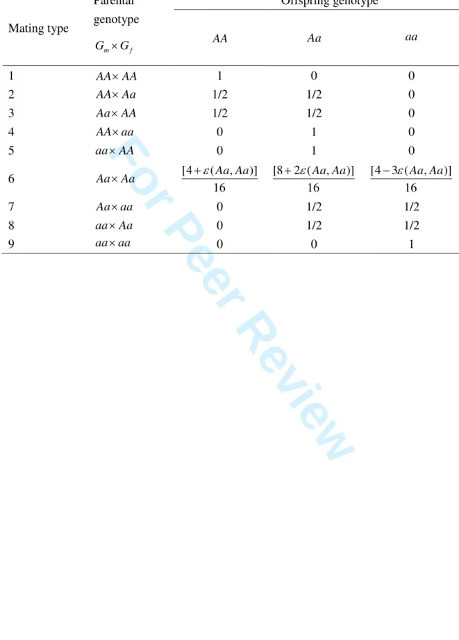
Table I. First-order approximations of the general CPG probabilities for the complete trio
under the null hypothesis of no association
Offspring genotype Mating type Parental genotype m f G ×G AA Aa aa 1 AA AA× 1 0 0 2 AA Aa× 1/2 1/2 0 3 Aa×AA 1/2 1/2 0 4 AA aa× 0 1 0 5 aa×AA 0 1 0 6 Aa×Aa [4 ( , )] 16 Aa Aa ε + [8 2 ( , )] 16 Aa Aa ε + [4 3 ( , )] 16 Aa Aa ε − 7 Aa aa× 0 1/2 1/2 8 aa×Aa 0 1/2 1/2 9 aa aa× 0 0 1 3 4 5 6 7 8 9 10 11 12 13 14 15 16 17 18 19 20 21 22 23 24 25 26 27 28 29 30 31 32 33 34 35 36 37 38 39 40 41 42 43 44 45 46 47 48 49 50 51 52 53 54 55 56 57 58 59 60
For Peer Review
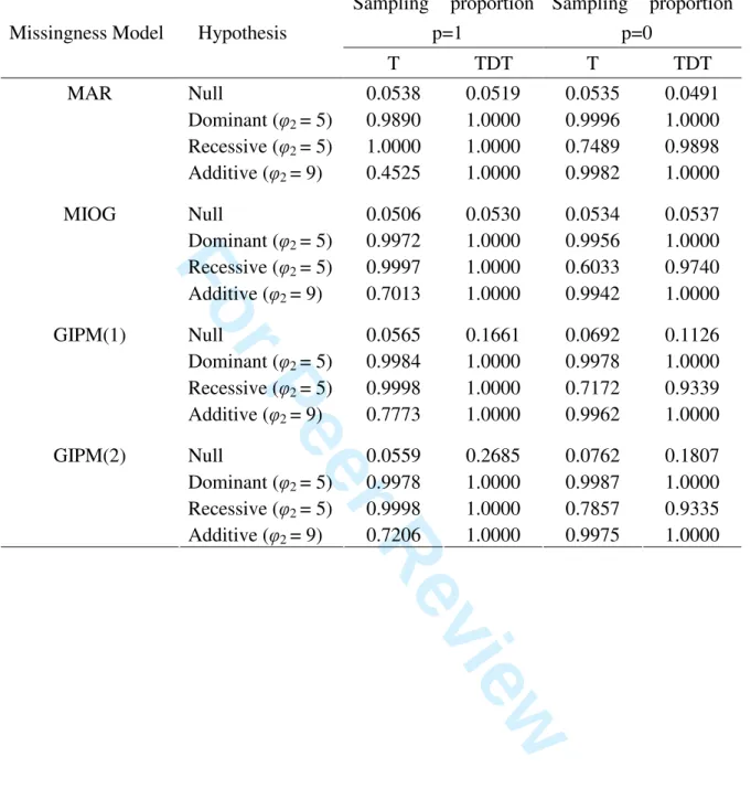
Table II. Sizes and Powers of the Association Tests Under One Population
Sampling proportion p=1
Sampling proportion p=0
Missingness Model Hypothesis
T TDT T TDT Null 0.0538 0.0519 0.0535 0.0491 Dominant (φ2 = 5) 0.9890 1.0000 0.9996 1.0000 Recessive (φ2 = 5) 1.0000 1.0000 0.7489 0.9898 MAR Additive (φ2 = 9) 0.4525 1.0000 0.9982 1.0000 Null 0.0506 0.0530 0.0534 0.0537 Dominant (φ2 = 5) 0.9972 1.0000 0.9956 1.0000 Recessive (φ2 = 5) 0.9997 1.0000 0.6033 0.9740 MIOG Additive (φ2 = 9) 0.7013 1.0000 0.9942 1.0000 Null 0.0565 0.1661 0.0692 0.1126 Dominant (φ2 = 5) 0.9984 1.0000 0.9978 1.0000 Recessive (φ2 = 5) 0.9998 1.0000 0.7172 0.9339 GIPM(1) Additive (φ2 = 9) 0.7773 1.0000 0.9962 1.0000 Null 0.0559 0.2685 0.0762 0.1807 Dominant (φ2 = 5) 0.9978 1.0000 0.9987 1.0000 Recessive (φ2 = 5) 0.9998 1.0000 0.7857 0.9335 GIPM(2) Additive (φ2 = 9) 0.7206 1.0000 0.9975 1.0000 3 4 5 6 7 8 9 10 11 12 13 14 15 16 17 18 19 20 21 22 23 24 25 26 27 28 29 30 31 32 33 34 35 36 37 38 39 40 41 42 43 44 45 46 47 48 49 50 51 52 53 54 55 56 57 58 59 60
For Peer Review
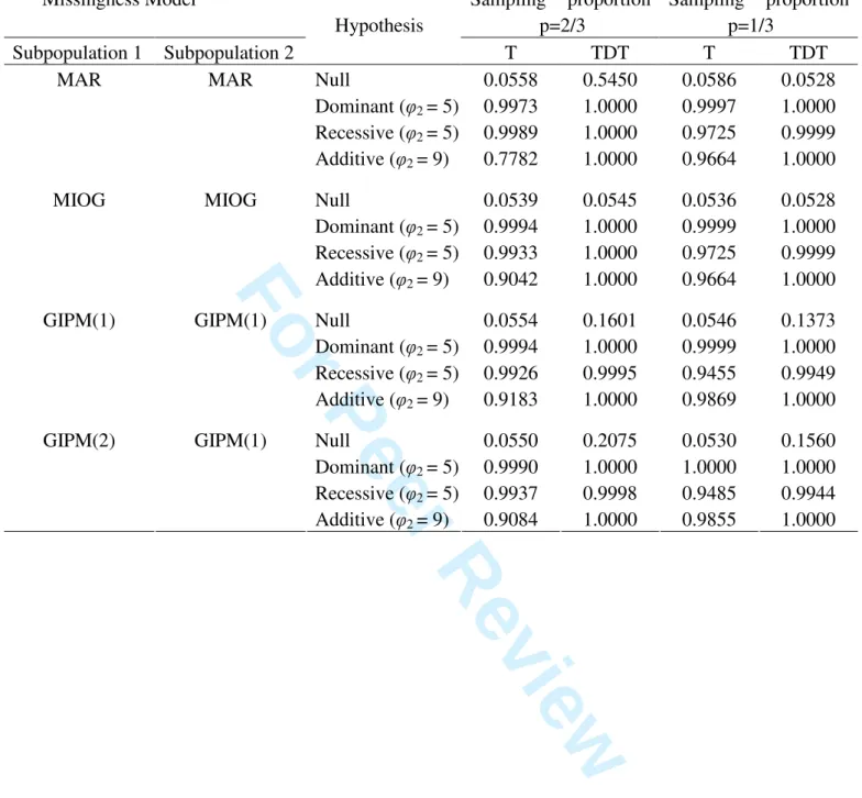
Table III. Sizes and Powers of the Association Tests Under Two Populations
Missingness Model Sampling proportion
p=2/3 Sampling proportion p=1/3 Subpopulation 1 Subpopulation 2 Hypothesis T TDT T TDT Null 0.0558 0.5450 0.0586 0.0528 Dominant (φ2 = 5) 0.9973 1.0000 0.9997 1.0000 Recessive (φ2 = 5) 0.9989 1.0000 0.9725 0.9999 MAR MAR Additive (φ2 = 9) 0.7782 1.0000 0.9664 1.0000 Null 0.0539 0.0545 0.0536 0.0528 Dominant (φ2 = 5) 0.9994 1.0000 0.9999 1.0000 Recessive (φ2 = 5) 0.9933 1.0000 0.9725 0.9999 MIOG MIOG Additive (φ2 = 9) 0.9042 1.0000 0.9664 1.0000 Null 0.0554 0.1601 0.0546 0.1373 Dominant (φ2 = 5) 0.9994 1.0000 0.9999 1.0000 Recessive (φ2 = 5) 0.9926 0.9995 0.9455 0.9949 GIPM(1) GIPM(1) Additive (φ2 = 9) 0.9183 1.0000 0.9869 1.0000 Null 0.0550 0.2075 0.0530 0.1560 Dominant (φ2 = 5) 0.9990 1.0000 1.0000 1.0000 Recessive (φ2 = 5) 0.9937 0.9998 0.9485 0.9944 GIPM(2) GIPM(1) Additive (φ2 = 9) 0.9084 1.0000 0.9855 1.0000 3 4 5 6 7 8 9 10 11 12 13 14 15 16 17 18 19 20 21 22 23 24 25 26 27 28 29 30 31 32 33 34 35 36 37 38 39 40 41 42 43 44 45 46 47 48 49 50 51 52 53 54 55 56 57 58 59 60
For Peer Review
317x171mm (96 x 96 DPI) 3 4 5 6 7 8 9 10 11 12 13 14 15 16 17 18 19 20 21 22 23 24 25 26 27 28 29 30 31 32 33 34 35 36 37 38 39 40 41 42 43 44 45 46 47 48 49 50 51 52 53 54 55 56 57 58KF Chenga,b, JY Leeb, and JH Chenc a
Biostatistics Center and Department of Public Health, China Medical University,bGraduate Institute of
Statistics, National Central University, Taiwan(ROC), andcBiostatistics Center and Graduate Institute
of Biostatistics, China Medical University, Taichung, Taiwan (ROC)
Short title: Assessing the Joint Effects of Population stratification and Sampling
Correspondence to: Professor KF Cheng, Biostatistics Center, China Medical University, Taichung,
Taiwan 40402, e-mail:[email protected], phone number: 886-4-2207-8539, fax number:
case-control studies producing spurious gene-disease associations. However, its impact on the study
of interactions is not clear. In this paper, we investigate the joint effect of population stratification
and sampling in case-control study of gene-gene or gene-environment interactions. We show that
the level of the PS bias in testing null interaction depends not only on the variations of the baseline
genotype (exposure) frequency, disease risk, and gene-gene (environment) odds ratio, levels of the
main effects, but also the sampling of the study. Using this result, we point out that the PS bias may
still exist even when the case and control data were matched in ethnicity. We also give general
conditions under which the PS bias is null and derive bounds for the bias when the structure of the
population is not known. The information about these bounds can be used to define conservative
tests. In this paper, we also quantify the PS bias to the genetic main effect and show how the bias is
modified by the presence of another factor. Finally, the performance of the usual tests is studied by
numerical examples.
Key words: bias; environmental risk factors; genes; interactions; population stratification; sampling
have been identified. Overwhelming evidence indicates that there are reasons to believe that relative
common polymorphisms in a wide spectrum of genes may modify the effect of environmental
agents [1, 2]. Several studies also have demonstrated the presence of gene-gene interaction in
complex human diseases [3-7]. Gene-gene interaction, epistasis, is also considered as a basic
genetic concept which has been widely used by biologists for a long time [8].
Many association designs have been proposed for studying gene-environment or gene-gene
interactions. Recently, Wang and Zhao [9] found that in the study of gene-gene interactions, the
unmatched case-control association design is more powerful than both the matched case-control
design and case-parents design. They also found that when a logistic regression model is fitted for
assessing gene-environment interactions based on case-parents sample [10], the approach may be
susceptible to the PS bias. However, case-control design is also well known to be susceptible to the
PS bias in the study of genetic effect, if the gene under study shows marked variation in allele
frequency across subgroups of the population and if these subgroups also differ in their base-line
disease risks [11-17]. Wang, et al. [18] recently provided numerical examples showing that when
the correlation between genetic and environmental factors is small or the linkage disequilibrium is
weak, and case-control data were collected according to a simple random sampling (SRS) scheme,
the PS biases in testing null interaction odds ratios are also small. However, the SRS scheme is
testing null interaction. We quantify the magnitude of the PS bias in terms of the baseline disease
risks, genotype frequencies (or exposure rates), their odds ratios (linkage disequilibrium
coefficients), the levels of the main effects, and sampling design used in the study. Based on this
result we are able to derive many important conditions under which the PS bias is null. We point out
that if the study does not follow an SRS design, the PS bias may be large even the genetic factors
under study are in linkage equilibrium. We also show that matching in ethnicity between case and
control samples cannot always eliminate the PS bias. However, our numerical examples indicate
that the biases are generally small when the genetic factors are in linkage equilibrium.
The PS bias often cannot be estimated, since wedon’tknow how many importantsubpopulations
involved in the studied population and/or which subpopulation a person belongs to. In this paper,
however, we are able to derive useful bounds to measure the maximal impact of the PS when the
structure of the population is not known. Sometimes, these bounds can be estimated so that more
careful conclusion about the significance of the test can be made; see Lee and Wang [19] for similar
suggestion in studies of gene-disease association. We give many numerical examples to show the
general performance of the usual tests.
In addition to the discussion about the PS bias in the study of interactions, we also discuss the
impact of the PS effect in testing the null genetic main effect when another genetic (environmental)
Methods
The Magnitudes of the Biases
We begin this section with the notation that will be used throughout this work. Disease status is
denoted as D with levels d=1, 0, indicating the presence and absence of the disease, respectively.
G=1 (0) represents the presence (absence) of the genotype of interest. H=1 (0) represents the
presence (absence) of the environmental exposure or another genotype of interest. All results shown
in this paper can be extended to any risk factor with finite number of levels. We let S denote a
general stratification variable with values s=1,…,K, representing K strata. S is not observable in
discussion of the effects of PS. In the subpopulation level, we assume that the risk model is given
by
logitP D( 1|Gg H, h S, s) s g h gh.
s=1, g=0, and h=0 represent the referent subpopulation, genotype and environmental exposure,
respectively. For identifiability purpose, we define 1 =0. s,s 1,...,K, are the subpopulation-specific parameters representing the potential heterogeneity of disease risk across
subpopulations. In this model, log-odds-ratio measures the association between the genotype
and risk of disease, log-odds-ratio measures the association between the environmental
s
OR to represent the corresponding baseline G H odds ratio (givenD0), G Hs( s)to represent the baseline G H( )-frequency odds (givenD0, andH G( )0), D to represent the baselines
disease frequency odds (givenH 0,andG0) and
* * ( | 1) ( | 0) ( | 1) ( | 0) s P S s D P S s D DS P S s D P S s D to
represent the deviation of the true sampling scheme of the study and the usual SRS scheme. Here
*
( | 1)
P S s D ( P S*( s D| ) is the true sampling proportion of the subjects from0) subpopulation s in the cases (controls), and P S( s D| 1) ( P S( s D| 0) ) are the corresponding proportions under SRS scheme.
Since in the population level we only observe factors G and H in a case-control study, we show in
the Appendix that the main effects and interaction are given by
D G odds-ratio =exp( *), DH odds-ratio =exp( ,*) G H interaction =exp( *), where * (1, 0) log (0, 0) K K , * (0,1) log (0, 0) K K , and * (1,1) (0, 0) log , (1, 0) (0,1) K K K K and * 1 * 1 ( 0, 0 | , 0) ( | 0) ( , ) . ( 0, 0 | , 0) ( | 0) k g h g h s s s s s s k g h g h s s s s OR G H D DS P G H S s D P S s D K g h OR G H P G H S s D P S s D
We note that if DsDSsis constant across subpopulations then there is no PS bias of any kind. A sufficient condition for this to hold is when the baseline disease risk is identical across all
The maximal impact of the PS bias to the genetic main effect and conditions for the null bias
The maximal PS bias to the genetic main effect depends on the variation of the baseline* genotype frequency odds, * max s min s,
s s
G G G variation of the sampling
deviation * max s min s s s
DS DS DS and variation of the baseline disease odds
*
max s min s s s
D D D . In the Appendix, we also showed that the bias can be expressed as
* exp( =)
1 1 1 k s s s s s k k s s s s s s s G D DS w G w D DS w
* * * * * * (1 ) , ( (1 ) )( (1 ) ) M M M m m m M m M M m m w G D DS w G D DS w G w G w D DS w D DS where w ands w* are some constants satisfying 0w*, ws 1and
1 1 K s s w
. The inequality shows that the bias is the greatest when the number of subpopulations is 2. Note that the value ofconstant w* is generally unknown, however, using the above inequality the bias can be shown to
be bounded above by
2 * * * * * * * * * * * * * * * 1 G D DS G D DS U G D DS G G D DS D DS .The bias is also bounded below byLU1. These bounds give the maximal impact of the PS in making inference about the genetic main effect. Under rare disease, the background disease rate is
if the data observed in the study follow an SRS scheme (DS*=1), and the disease risk is constant,
then the PS bias is also null. (However, if the sampling is not SRS, the results in Tables 1-2 show
that the PS bias may be non-null even when the subpopulations have constant disease risk); (3) if
the case and control data were matched in ethnicity, and H-main effect and interaction are null,
then there is the PS bias is null. (However, if there is non-null H-main effect (or non-null
interaction), the results in Tables 1-2 show that the PS bias is non-null)
The maximal impact of the PS bias to the interaction and conditions for the null bias
The PS bias to the interaction effect also depends on the variation of the baseline odds ratio*
*
max s min s.
s s
OR OR OR We point out that OR* is not necessary to be 1 even the two genetic factors are in linkage equilibrium within each subpopulation. In fact, if the latter condition holds,
one can show
1 exp(1 exp() 1 exp(
) 1 exp( ) )
,s s s s s OR where ( 0 | ) log . ( 0 | ) s s P D S s P D S s
Thus, OR* also depends on the levels of the main effects and interaction. In the Appendix, we
showed that under SRS, the bias was bounded above by (1) *2
U D and bounded below
(1) *2 1
( )
L D . These are the same bounds derived by Wang et al. [18]. Unfortunately, these bounds are not valid if the SRS condition is not satisfied. Under general sampling design, we showed that
and bounded below by 1 U(2) L(2) . We note that if the genetic factors are in linkage equilibrium within each subpopulation, and the G(orH)-main effect is null, then OR* 1in testing null interaction. Under this scenario, if the variation of the G(orH) frequency odds is small, the above
bounds show that the bias of the test cannot be expected to be large.
Using these bounds, some interesting conclusions about the PS bias can be reached: (1) if the
baseline G H odds ratio and G(orH)- frequency odds are constant across subpopulations then the PS bias is null; (2) if the sampling of the study is SRS, and the disease risk is constant, then* the PS bias is also null. (However, if the SRS condition does not hold, the latter conclusion is not
necessary valid; see Tables 1-2 for more results.)
RESULTS
True type I errors
In case-control studies, one often expects that the type I errors of the association tests can be
approximately controlled at some predetermined level. However, in the presence of PS, the usual
test statistic does not have a chi-square distribution under null hypothesis. Instead, it has a
non-central Chi-square distribution, with non-centrality parameter depending on the level of the PS
bias. Thus, the usual chi-square test tends to have inflated type I errors.
Suppose that the intended type I error rate of the chi-square test is and let 1;12represent
given by
2 * (1) (1) (1) (1) (0) (0) (0) (0) 11 01 10 00 11 01 10 00 . 1 1 1 1 1 1 1 1 ( ) ( ) n n n n n n n n where n( )ghd is number of observations with outcome Gg H, h and disease status d. Then the true type I error of the usual chi-square test of null interaction is given by P(12( ) 1;12), which is always greater than or equal toIn the case of testing null genetic main effect, the.
non-centrality parameter is given by
2 * (1) (1) (0) (0) 10 00 10 00 log( ) . 1 1 1 1 ( ) n n n n The corresponding true type I error of the chi-square test is given by P(12( ) 1;12), which is also.
Tables 1 and 2 show values of the PS bias, bias* and true type I errors of the usual* chi-square tests when the significance level is 0.05. We assumed that there are two subpopulations
(K 2), 0,0or 1 (thus OR =1 under linkage equilibrium),s G(H) frequency of the first subpopulation was given by P G( 1|S 1) 0.51 ( P H( 1|S 1) 0.19) , the first subpopulation disease risk was P D( 1|S 1) 0.05, the proportion of subpopulation 1 in the overall population was 0.7, and case and control sample sizes both equaled to n= 500. We defined
1 2
( , ),
parameter values were determined from the variations G H D and*, *, * DS*given in the tables with the assumption that subpopulation 2 has the maximal baseline G(orH) frequency odds, disease
risk, and sampling deviation (this implies that P S*( 2 |D ranges from 0.0585 to o.7163).0) Finally, we note that in computing the non-centrality parameters, the sample frequencies d
gh
n were
replaced byn P G ( g H, h D| .d)
According to the results in Table 1, the true type I error ranges from 0.05 to 0.9998 under linkage equilibrium. If the SRS condition holds and0, the true type I error ranges from 0.05 to 0.9602 with mean 0.4377 and standard error 0.3298. Under the same scenario but1, the corresponding range becomes (0.05, 0.9326) with mean 0.3822 and standard error 0.2969. On the
other hand, if the sampling is not SRS (DS*=3 or 5) and0, the range of is (0.05, 0.9998) with mean 0.4747 and standard error 0.3978. Under non-SRS but 1, the corresponding range becomes (0.05, 0.9992) with mean 0.4425 and standard error 0.3678. These summarized results
indicate that the PS bias can be quite large and its level may be modified by the sampling design
and the level of H-main effect. In general, the PS bias is smaller when 1. We also observed that the PS bias may be non-null under perfect matching. For example, if the matching is perfect* and H-main effect 1, the largest true type I error is 0.1064, which occurs at the case with
* * *
5.
G H This is contrary to our usual believe that matching between cases and controlsD
disequilibrium coefficient is small and the sampling is SRS. Our Table 1 also shows that under SRS
and linkage equilibrium, the true type I error in testing null interaction ranges from 0.05 to 0.0659. This agrees with the finding by Wang et al. However, if the sampling is not SRS (DS*=3 or
5), has range (0.05, 0.2656), mean 0.0840, and standard error 0.0516 when 0, and range (0.05, 0.2750), mean 0.0871, and standard error 0.0550 when1. These results indicate that PS also can cause serious problem in case-control study of gene-gene interactions even the two genes
are in linkage equilibrium. Under this scenario, the best way of reducing the bias is to match cases
and controls in ethnicity. We note that under perfect matching and linkage equilibrium, the range of
is only between 0.05, and 0.0541.
Linkage disequilibrium between two genes or correlation between genetic and environmental
factors also play important role in determining the PS level in the studies of interaction. According
to results presented in Table 2, we find that the bias to the genetic main effect becomes smaller
when the linkage disequilibrium coefficient increases to 0.05. When 0, the mean of is 0.3377 under SRS and 0.3843 under non-SRS, and when 1 the mean becomes 0.2716 and 0.3351, under SRS and non-SRS, respectively. On the contrary, the bias to the interaction effect
increases when the linkage disequilibrium coefficient increases to 0.05. Our results show that
when0, the mean of is 0.1642 under SRS and 0.3841 under non-SRS, and when 1, the mean becomes 0.1706 and 0.3906, under SRS and non-SRS, respectively. In all, the PS bias *
perfectly matched.
Discussion
The impact of population stratification is considered by many to be important in case-control
studies of gene-disease association. Many authors have suggested quantitative methods to control
type I errors of the usual association test. The most popular treatments include the “genomic control” method [17, 21-26] and the “structure association” method [20, 27- 30]. Each of the
proposed methods requires typing extra polymorphic markers to generate an estimate of PS bias
which can be used to adjust the test statistic. The impact of PS in case-control studies of gene-gene
(environment) interaction is considered to be less important, when the genes under studied are in
linkage equilibrium or when the gene-environment correlation is weak [18, 31]. However, this
conclusion holds only when the sampling of the case and control data follows a simple random
sampling design. Unfortunately, there exists no formal test for testing the validity of the SRS
condition when the PS is present.
In practical applications, the SRS condition is rarely satisfied. For examples, when the
hospital-based cases (controls) are used in the study and they are not representative of the
population-based cases (controls) or when the non-response of the cases or/and controls occur in the
study, then the SRS condition may fail. In this paper, we show that under slight deviation of the
genetic factors are in linkage equilibrium or when the genetic and environmental factors are
uncorrelated. Large correlation or strong linkage disequilibrium could make the PS bias become
even larger. Also, small variation in disease risk cannot guarantee small PS bias to the interaction,
unless the sampling of the study follows an SRS design. Therefore, in applications, it is also
important to be able to measure the maximal impact of the PS bias. In this paper, we drive bounds
for the PS bias. If the bounds are estimable, then they can be used for making more conservative
inference.
We note that matching in ethnicity between cases and controls has been suggested by the
epidemiologists to control the PS bias in case-control gene-disease association study. However, the
PS bias () to the genetic main effect also depends on the sampling design and levels of another* main effect (value) or interaction effect. We found that if 0 then the residual bias to the main effect after matching is zero. However, if1, and0, the residual bias may still be substantial. Tables 1-2 also show that matching cannot remove the PS bias to the interaction effect.
However, under the cases considered, the biases are small.
Since the presence of PS may cause unacceptable bias to the usual interaction analysis, it is of
importance to have an efficient method to control the bias. Unfortunately, so far there exists no
effective method for controlling the PS bias in the studies of interaction. The major difficulty is that
wishes to test the significance of the gene-gene interaction, the genomic control method may be
applied to control for the PS bias. One can follow the idea of genomic control to type extra pairs of
null markers and apply the computed interaction levels to control the PS bias. In principle, if the
candidate markers are in linkage equilibrium, the selected pairs of null markers also need to be in
linkage equilibrium so that the important characteristics of the PS bias can be captured. On the other
hand, if the candidate markers are in linkage disequilibrium, the paired null markers also need to be
correlated. We are currently working on this important problem. Another approach is to reduce the
PS bias by matching the cases and controls in the study. We find that under perfect matching and
linkage equilibrium, the PS biases to the interaction effect are small in the discussed cases. More
study is needed in order to understand the impact of the residual bias when matching is not perfect.
Finally, we point out that one may also use extra null markers to determine the number of
subpopulations involved in the study and identify which subpopulation a person belongs to and use
this information to fit the risk model. However, the success of this approach also heavily depends
on the selection of the null markers.
Appendix
Following the usual Bayesian argument, the disease-risk model implies that
Pr Gg H, h S| s D, 1 Pr Gg H, h S| s D, 0 exp
s g e ge
, where s slog Pr
D0,S s
Pr D1,S s
, s=2,…,k. As a consequence,On the other hand, the joint frequency distribution of G and H in the control population is given by
*
1 Pr , | 0 Pr , | , 0 P | 0 . k s G g H h D G g H h S s D S s D
Thus their ratio is given by
* * * * * Pr , | 1 Pr , | 0 exp , exp . G g H h D G g H h D g h gh K g h g h gh Here, we define *
*
log K 0, 0 ,
* * * 1, 0 log 0, 0 K K ,
* * * 0,1 log 0, 0 K K and
* * * * * 1,1 0, 0 log 0,1 1, 0 K K K K , where
* * 1 * 1 Pr , | , 0 P | 1 exp , . Pr , | , 0 P | 0 k s s k s G g H h S s D S s D K g h G g H h S s D S s D
It can be shown that *
represents the PS bias to the genetic (environmental) main effect,* and is the PS bias to the interaction effect. We note that*
( 0 | 1, ) exp ( 0 | 0, ) s P G H D S s P G H D S s ( 1| 0, ) ( | 0) ( 0 | 0, ) ( | 1) P D G H S s P S s D P D G H S s P S s D ( 0) , ( 1) P D P D thus one can re-write *
, ( , ) ( 0). ( 1) P D K g h K g h P D where * * 1 ( 0, 0 | , 0) ( | 0) ( 0, 0 | , 0) ( | 0) s k s P G H S s D P S s D w P G H S s D P S s D
.Simple algebra shows that thereexists some constant w*such that the bias is bounded above by
* * * * * * (1 ) ( (1 ) )( (1 ) ) M M M m m m M m M M m m w G D DS w G D DS w G w G w D DS w D DS 0 1 (1 ) max ( (1 ) )( (1 ) ) M M M m m m w M m M M m m wG D DS w G D DS wG w G wD DS w D DS
2 * * * * * * * * * * * * * * * 1 . G D DS G D DS G D DS G G D DS D DS Also note that under SRS, DSs and therefore according to the definition of1 exp( , we*)
easily show that it is bounded above by D*2and bounded below byD* 2. However, under general sampling design, the bias is expressed as
* 1 1 1 1 1 1 exp( ) , k k k s s s s s s s s s s s k k k s s s s s s s s s s s OR G H w G w H w G w H w OR G H w
where * * 1 ( | 0) ( | 0) s s s k s s s D DS P S s D w D DS P S s D
, * * 1 ( | 0) ( | 0) s k s P S s D w P S s D
. By applying the sameapproach for deriving bounds forexp( , we also can derive bounds for*) exp( .*)
Acknowledgements
This research was supported in part by a grand from National Science Council and a joint research
grand from China Medical University and Asia University.