Nonlinear adaptive control of a flexible manipulator for automated deburring

Proceedings of the 1997 IEEE

International Conference on Robotics and Automation Albuquerque, New Mexico - April 1997

NONLINEAR ADAPTIVE CONTROL

O F

A FLEXIBLE

MANIPULATOR FOR AUTOMATED DEBURRING

Ling-Hui Chang and Li-Chen

Fu

‘9’

Department

of

Electrical Engineering’

Department of Computer Science and Information Engineering’ National Taiwan University

Taipei, Taiwan, Republic

of

China

Abstract: The goal of the automated deburring can be achieved by maintaining a constant force on the grinding tool in the direction normal to the constraint surface while following the positional trajectory in the direction tangential to the surface. In this thesis, the dynamics of both the deburring process and the flexible manipulator will be investigated in detail, and a singular perturbation technique is then utilized to separate the system into a slow subsystem and a fast subsystem, whereby an adaptive hy- brid position/force controller is derived for the slow subsystem whereas a dynamic feedback controller is developed for the fast subsystem. It is shown that the motional tracking error and the force regulation error will both converge to a small residual set. Finally, the computer simulations and experiments of a 2-link flexible manipulator confirm the effectiveness of the proposed controller.

1.INTRODUCTION

In most occassions, where parts need to be assembled properly and safely, the burrs on the part’s edge must be removed. However, the manual deburring process is a costly and time-consumming operation. For reducing the manufacturing cost efficiently, automated robotic deburring systems will naturallly be considered as a good solution and, hence, is investigated thoroughly in this thesis.

In an automated robotic deburring process, the grinding tool mounted onto the end-effector must make a contact with the part’s edge. Since both the robot manipulator and the part are mostly rigid, the impact from the manipulator to the part will frequently cause damage to each other. Besides, due to the shortcomings of applying conventional rigid robot manipulators, such as high-power consumption, low motion speed and low payload ratio, the research on controlling the flexible manipulators has attracted more and more attention nowadays.

In recent years, there have been many reaserch re- sults on the automated robotic deburring reported. In [ 2 ] , the control approach proposed there is to main- tain constant normal force and tangential force by the impedance control. An alternative approach is to con- trol the chamfer depth with the minimal surface by minimizing the normal cutting force [3].

From a different view-point, a more advanced control method, teaching and learning of adaptive control has been proposed for automated deburring [4]. In [5], the sensing system combines the information from foece

and vision sensors to measure the chamfer depth, and the chamfer depth is controlled based on an adaptive predictive learning control stratege.

However, for constrained flexible manipulators, there are some results which have been presented. Mat- sun0 et al. [7] have proposed a hybrid position/force controller based on the quasi-static equations. Lian et al. [l] proposed an adaptive hybrid position/force controller based on singular perturbation theory for flexible manipulators in Cartesian space. Rocco and Book [8] presented a reduced order model of a flexible robot and a sigular perturbation vesion of the model is also given, whcih shows some differences from pre- vious results. Kim et al. [9] presented a hybrid po- sition/force control scheme to a flexible manipulator using a lumped-parameter modeling.

In this thesis, a deburring process model is presented, and a reduced model in Cartesian space is derived due to the constraints imposed on the end effector. Base on sigular perturbation theory, an nonlinear adaptive controller is designed for the system. In our Advanced Control Laboratory (ACL) at National Taiwan Uni- versity (NTU), a 2-link planar flexible manipulator equipped with a grinding tool has been built to demon- strate the performance of the proposed controller.

This thesis is organized as follows : Section 2 present the model of the deburring process and the dynamic model in task space of a constrained flexible manipu- lator. Further by applying the singular perturbation technique, the original system is decomposed into a slow subsystem and a fast subsystem. In Section 3, a nonlinear adaptive controller is developed based on the This research is sponsored by National Science Council, R 0 C , under the grant NSC 85-2212-E-002-078

Normal

Figure 1: T h e burr cross-section

formulation of the two subsystems derived previously. and the simulation result will be shown. In Section 4, the experimental result will demonstrate the real con- trolled performance. Finally, some conclusions will be given in Section 5.

2.PROBLEM FORMULATION

Deburring Model

In the process of deburring a part’s edge by a flexi- ble manipulator, the end-effector of the manioulator equipped with a grinding tool will remove the burrs by cutting at a constant chamfer depth into the nominal edge of the part while moving along the part’s actual edge under a feedrate. There exists an interaction force between the end-effector and the surface of the edge, called the cutting force, which can be decomposed into a force in the direction along the constraint surface and another in the direction normal to the constraint sur- face. According [2], we will introduce the model of the deburring process in the following.

First we give some general descriptions of the ge- ometric characteristics of burrs. Fig. l shows the cross-section of a burr, from which burr height, burr thickness, and the chamfer depth are clearly illustrated. Here, we assume that the average burr height is much greater than the average burr thickness [2].

A three-dimentional geometric model of a cutting surface is shown in Fig. 2. Let the cutting area be projected into the plane tangential to the constraint surface and another plane with a normal tangent to the same surface, respectively. We can see that each of the projected areas can, in fact, be decomposed into two parts, one from burr projection and the other from chamfer projection. According to the previous assump- tion, i.e., the burr height is much greater than the burr thickness and the chamfer depth is usually chosen to be greater than the maximum of the possible burr thick- ness, the normal projected area of the burr relative to the normal projection of the contact area can be very insignificant, but the tangential projected area of the burr relative to the tangential projection of the con- tact area becomes much more substantial. It means that the variation of the tangential projected area with the burr size is much greater than that of the normal projected area with burr size.

Figure 2: The 3D geometric model of the cutting sur- face

Intuitively, the cutting force is proportional to the contact area. Accordingly, it is sure that the tangential forcee varies much more significantly with the burr size, but the normal force maintains almost constant magni- tude regardless of the burr size. Therefore, a consistent chamfer depth can be obtained by controlling only the normal force.

In the following, we will derive the tangential cutting force in detail. According t o [2], the material removal rate M R R can be expressed as:

M R R

=

( A ,

+

Ab) x V t ₍₁₎ where A , and Ab denote the cross sectional area of the chamfer and of the burr, respectively, and vt is the velocity of the grinding tool along the part’s edge.

In the deburring process, the tangentail cutting force is proportional to M R R . Then, according to (l), the relationship between the tangential cutting force and the tangential velocity can be expressed as:

ft = ( k t

+

A h ) x U t ₍₂₎ where kt is a posive constant, and Akt is an uncertainty

from the variation of the burr size. For a large tangen- tial force, there may exist some problems, such as the grinding tool may be stalled and quickly wears out.

To avoid the above problems, for a given desired cut- ting chamfer depth, we can select a desired feedrate which does not yield a large tangential cutting force but makes the grinding tool work normally. If the burr size is much smaller than the chamfer depth, this ob- servation will be even more justified. Finally, it should be realized that one can use position control in the di- rection tangential t o the constraint surface and force control in the direction normal to the same surface in order to accomplish the above-mentioned control task in the deburring process.

Dynamic Model of

a

Deburring Flexible

Manipulator

in

Task Space

Recall the discussions in the previous section, con- cerning an end-effector of a flexible manipulator which

moves along the part's edge for deburring. There exists an interaction force called the cutting force between the end-effector and the surface. The dynamic model can be expressed as

where qr E R", (n

5

6) and qf E R " f , n

+

nf = N , X E R" is the vector of Lagrange multipliers assc- ciated with the geometric constraints @'(q) = O , @ : RN -+

R",

A1 =

e,

A2 =

E ,

and rt E

RN

denotes the tangential cutting force in joint-space coordinates. The subscript T and f denote the rigid mode part and flexible mode part, respectively.

Owing to task requirement, a dynamic model in Cartesian space would better be derived. First, we de- note I as the position of the end-effector in Cartesian space, and I can be expressed as I = X ( q ) , where

X

: RN --+ R", qT = [ q T , q 7 l T . Then,

and

[;;I=[

$ ] f t

ax

where Jr =

e,

JJ =

G,

and f t E

R"

is the tangen- tial cutting force in Cartesian space. Assume that the flexible manipulator is non-redundant with respect to the rigid part so t h a t Jr is insured to be invertible. As a result, we can obtain the dynamic equations in the task space as follows:

And the flexible part can be expressed in a more com- pact form as follows:

To tackle the problem with vibration suppression, we will apply the singular perturbation theory here and separate the flexible manipulator system into a slow subsystem and a fast subsystem. To that aim, we make the following definition first :

U = I C q f , and

k

= ICE',

where c2 is a common factor extracted from each entry

of the matrix IC', assumed to be small enough. Next, we define the state variables : 21 = v and 2 2 = c l j ,

y1 = I and y2 = i. so t h a t , acccording to (7) and (S),

the state space form of a singualr perturbed model can thus be derived as follows:

Y1 = Y2 (9)

€21 = 22 (10)

y2 = Diy2

+

E D Z ~ - ~ Z ~

+

0 3

+

0 4 2 1

+

D S T

+

D6

€22 = K ( E l y 2

+

€EZk-'zz

+

E3

+

E 4 Z 1

+

E57

+

E6)

For the extreme case where E + 0, we can obtain the following relation via (IO) :

zz

= 0

r1 =

-Eil[Eiyz

-I- E3 4- E57

+

EG],

(11) which can be subsituted into (9) with E = 0 t o yield the following set of equations :

Y 1 = Y2

5,

=

[Jr

-

&M;1Crr]J32

-

j r M ; l G 1

+

JrM,,'?

+

JrPMT;l(ATS;

+

J 7 5 )

(12)

where we have used the additional relation Mrr =

( H I 1

-

H~~H,;'Hz~)-', and all the variables and func- tions with overbar are used to denote those in (9), (10) in the situation when E = 0

.

This system will then be referred to as the slow subsystem.

For deriving the fast subsystem, we first define the fast time-scale as p

=

$

and then redefine the fast

variables as 71 = z1

-

21 and 72

=

zz

-

22.

As E --+ 0, we can obtain

9

=

%

= 0, which implies that y1 and yz are constants with respect to the fast time-scale p , i.e., within the boundary layer,

y1 and y2 are stationary. Therefore, the fast subsystem can be easily derived as

= 172

d7]1

dP

dP

d7]2

= -kHz271

+

R H ~ ~ ( T

-

T ) (13) Next, due to the existing constraints, W ( q ) = @(z) =

0, where @ : R" -+ R". Further, we will derive the original equations of motion into a reduced set of equa- tion. First, we separate the state 3, in the slow subsys- tem into two parts, namely, f l and 2 2 , where 21 E R" and 22 E R"-", so that the constraint can be further rewritten as: &(f) = 21

-

a(?,)

= 0, where

a

is a nonlinear map form R"-" to R". Of course, the total m constraint equations from @(I) = 0 are functionally

independent.

Then, we rewrite the state-space equation (12) into a set of differential equations, by premuliplying the equa- tions by

j;'Mrrj;'.

then the resulting equations be- come:

where

(15)

where F2 =

e,

$1 is the component of the tangential force in 5 1 direction, and f t 2 is the component of the tangential force in 22 direction.

Now, if (14) is used to replace 5 1 , &,

&,

and premul- tiply the second equation in (14) by

Fr

and add the result to the first equation in (14) to eliminate -F2x in the second equation, we can obtain the following set of equations:

fil&

+

CI&

+

GII = f1

+ +

ftl(l8) f i 2 &

+e&

+

F 2 G 1 1 + G I 2 = F:f1+ f2

+

I”ftl+

f12(19) Similarly, we can also refer the equations (18) and (19) as force part and motion part, respectively.

3.CONTROLLER DESIGN

Slow Subsystem Controller

Before we discuss the controller design, we will summa- rize some properties of the slow subsystem (18), (19) described in the previous chapter.

Proposition 3.1 : A?f2 is symmetric and positive def-

inite.

Proposition 3.2 : By a proper choice of C(q, q ) t o de- fine C 2 in (19), the matrix h2-2C2 is skew-symmetric.

Proposition 3.3 : There exist some constant system parameter vectors 8 1 and 82 such that

M 1 u + C 1 u - G 1 1

=

W T e , (20) B Z l F 2

+

&)U

-

G l 2 ( M 2 1 F 2

+

M 2 2 ) G

+

(MZlFZ

+

= w p 2 , - (21) Mzzi

+

C 2 u

+

F:&+

G I 2 =

{F:.T

69

[

;;

]

=

W T e , (22)

where U is a smooth variable with proper definition and

W l , Wz, and

w

are known functions matrix.

Proposition 3.4 : The uncertainty of the tangential force can be bounded as follows :

IIF2Tftl

-

F , T f t I

+

f t z

-

it211

<

P112;11

where

p

>

0 and 52 is the component of the velocity of the end-effector in x 2 direction.

Now, we are ready t o introduce the design of the hy- brid adaptive position/force controller in the following.

First, we define an error signal as

&

= 5 2

-

X 2 d . Then we define an auxiliary signal 3 as S

=

%Z

+

Kr&, where

Kr

>

0. Let the control law be designed as: fl =

-

w 1 0 1 - T -

+

IE

-

h l f2 = -wf8,-F:IC-KpS

- K ~ l l & l l s s n ( q - i t 2 (23) where n

=

K j ( x - A d )

-

x , K j

>

0, and K p

>

0,

K ,

>

0, and

8j

denotes the estimate of the vector of system parameters

8j,

i = 1 , 2 . Let the adaptation law be designd as:

where

r

>

0 and U

>

0.

According t o Proposition 3.1, 3.2 and 3.3, equation (18), (19) and the control law (23) the error dynamics involving i can be derived as follows :

M z k

+

f?23 = CTZ

+

FFftl- F T f t 1

+

$2

-

ft2 - K p 3

-

I‘,ll.&llsgn(S) (25)

MlS’+C,S =

w T i l + K f i + f i l - j t l ,

(26) where =

8

-

e

is the parameter estimation error and

=

x

-

A d is the force tracking error. The control

results of the slow subsystem are summarized in the following theorem.

Theorem 3.1: Consider the slow subsystem (18)-

(19) with the control law (23) and the adaptation law (24). Then, all signals inside the system remain bounded and both tracking errors in position and con-

tact force will converge into a residual set.

Proof: Let the Lyapunov function candidate as:

(27) and then take its time derivative along the trajectories of (25) to obtain

1 1

I

-Am(Kp)ll#

-

,ull~ll2

+

~“118112

5

-711k112 7 0 (28)

-

where ( = [I

81,

7 0 and 7 1 are positive constant, and Am(ZC,) and &(lip) denote the smallest and the

largest eigenvalues of IC,. Note that there exits K , such that A,(K,)

-

/3 is positive definite matrix.

Therefore, we can guarantee that S and

8

are bounded, and so are

&,

2 2 by use of a Lyapunov the- orem. Consider the closed-loop dynamical equation (25),

s'

is obviously bounded. According to (26), we get the force error

x

to be expressed as:

-

which readily implies that

i

is bounded. If K f is large enough, then the force error can even be made arbi-

trayrily small. 0

Fast Subsystem Controller

Now the fast subsystem (13) is rewritten in a very com- pact form as follows :

Within the boundary layer the system matrices

A

and

B

can be replaced by

A O

+

A& and

BO

+A&,, re-

spectively, where

&

and

&

are nominal matrices with known elements and there are availabe known bounds on llA&ll and llA&/l.

Here, after a careful study, a proper design of the aforementioned regulator is apparently a dynamic feed- back controller expressed as follows :

where the matrices

E

and G will be determined later. By adopting such control, the closed-loop fast subsys- tem becomes

where

6

= [qT,

T T ] ~ ,

A

=

,

and

B

=

[

1.

The following theorem summarizes

a condition under which the above design of the fast

subsystem controller may provide the desirable result.

Theorem 3.2: If and G are chosen such that A is Hurwitz and there ezist P,

Q

>

0 satisfying

1

j0 Bo

I

A T P

+

P A =

-&

(33)

and Amin(&)

>

~cYIIPII, where llBll

5

Q, then it is guar-

Proof: The proof is omitted here due to limited space. One can see [lo] for details.

anteed that

ll<ll

-* 0 ezponentially.

*

Composite Controller:

Consider the original system (7)-(8) with the control law r = ?

+

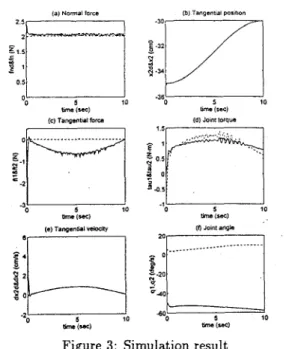
r f . The control results of such system are detailedly summarized in the following theorem.

(a) Normal force C . ... 0

!::m

10 OM IMI %

Figure 3: Simulation result

Theorem 3.3: Consider the system (9)-(10) with the composite control law (23), (31) and the adaptation law (24). Then, all signals inside the system remain bounded and both tracking errors in position and con-

t a c t force and link vibration will converge into a resid- ual set of a site which is an order of e , provided e is sufficiently small.

Proof: The proof is omitted here due t o limited space.

One can see [lo] for details.

Simulation Result

A computer simulation results of a case of a 2-link plan- nar flexible maipulator deburring system will be shown to verify the performance of the previous design of the composite controller. Assume that the gravitational force and the torsion effect of link can be neglected.

Here, we use 2 modes to describe each link's deforma- tion. The constaint surface is set as X I = 0.85m, and

the desired positional trajectory and force trajectory are chosen as follows :

The simulation results are shown in Fig. 3. Fig. 3

(a) (b) show the normal cutting force and tangential postional tracking trajectories, respectively, Fig 3 (c)

shows the tangential cutting force, and Fig. 3 (d) shows the input torques. From these figures of the simulation results we know that the tracking errors converge and all system states and control inputs are bounded simu- taneously. Therefore, the effectiveness of the composite controller is verified.

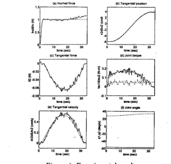
4 . E X P E R I M E N T A L RESULTS

~a [M) bnu (sec)

Figure 4: Experimental result

tem has been set up and experimented in Department of Electrical Engineering at National Taiwan Univer- sity (NTU). T h e 2-link flexible manipulator is drived by two revolute joints which are perpendicular to the motional plane. The first link is driven by a D.C. mo- tor with ratio 128:1, and the second link is driven by a

D.C. Brushless motor with gear ratio 1 O O : l . There is

a grinding tool equipped at the tip of the second link and the second joint of the manipulator is air-based in order to counteract the gravity. In the experiment, the flexible modes are measured using strain gauges. A PC

486-33 is used as the processor to implement the com- putation of the control law and the adaptation law, in which the sampling rate is set to be 300 Hz.

The workpiece chosen for deburring is a rectagulat steer slip, which is held paralel to the y-axis direction int the task space. The constraint surface of the work- piece can be mathematically represented as z = 0.9. The experimental results are shown in Fig. 4 , which are the control results with different feedrate. Fig. 4 (a) (b) show the normal cutting force and tangential pos- tional tracking trajectorie, respectively, Fig 4 (c) shows the tangential cutting force, and Fig. 4 (d) shows the input torques. From these figures of the experimental results, the preformance of the composite controller is verified.

6.CONCLUSION

In this thesis, the deburring model was presented and the dynamic model of an n-link constrained flexi- ble manipulator in task space was derived. A general method, namely, the singular perturbation method was utilized to formulate this problem into a two time-scale system in Cartesian coordinate. According to the nat- ural characteristics of the constrained system, we can further reduce its slow subsystem into an even simpler

one. Under this formulation, a nonlinear adaptive con- troller is then proposed. The tracking errors of position and force as well as the link vibrations can be shown

to converge to a small residual set.

To demonstrate the effectiveness of the nonlinear adaptive controller proposed, both computer simula- tions and the actual experiment were both performed. All the results obtained indeed manifest the promising potential of real application.

References

[I] Lian, F. L., J. H. Yang and L.

C.

Fu, “Adaptive hybrid position/force control for flexible manipu- lators in task space, ” Proc. National Symposium

on Automatic Control, pp. 210-214, 1995. [2] Kazerooni, H., J. J. Bausch and B. B. Kramer,

“An approach to automated deburring by robot manipulators, ” A S M E J. Dyna. Syst. Meas.

Contr., vol. 108, pp. 354-359, Dec. 1986.

[3] Bone G. M., M. A. Elbestawi, R. Lingarkar and L. Liu, “Force control for robotic deburring, ” A S M E

J. Dyna. Syst. Meas. Contr., vol. 113, pp. 395-400, Sep. 1991.

[4] Liu, S. and H. Asada, “Teaching and learning of deburring robots using neutal networks, ” Proc. of

1993 IEEE, pp. 339-345, 1993.

[5] Bone, G. M. and M. A. Elbestawi, “Sensing and control for automated robotic edge deburring, ”

IEEE Trans. Industrial Electronics, vol. 41, no. 2, pp. 137-146, April 1994.

[6] Matsuno, F., T. Asano and Y. Sakawa, “Modeling and quasi-static hybrid position/force control of

constrained planar two-link flexible manipulators,

” IEEE Trans. Robotics Automation, vol. 10, no.

3, pp. 287-297, June 1994.

[7] Matsuno F., T. Asano and Y. Sakawa, “Modeling and quasi-static hybrid position/force control of constrained planar two-link flexible manipulator,”

IEEE Trans. Robot. Automat., vol. 10, no. 3., pp. 287-168, June 1994.

[8] Rocco P. and W. J. Book, “Modeling for two-time scale force/position control of flexible robots,”

Proc. IEEE Int.

Conf.

on Rob. and Autom., pp.

1941-1946, 1996.

[9] Kim J.-S., K. Suzuki, A. Konno and M. Uchiyama, “Force control of constrained flexible manipula- tor,” Proc. IEEE Int. Conf. on Rob. and Autom.,

pp. 635-640, 1996.

[lo] Chang, L.-H, “Nonlinear adaptive control of a flex- ible manipulator for automated deburring,” Mas- ter Thesis, Institute of Electrical Engineering, Na- tional Taiwan University, Taiwan, R.O.C., 1995.