Dynamic response of soft poroelastic bed to nonlinear water waves — a boundary layer correction approach

(1)

D

YNAMIC

R

ESPONSE OF

S

OFT

P

OROELASTIC

B

ED TO

N

ONLINEAR

W

ATER

W

AVE

—B

OUNDARY

L

AYER

C

ORRECTION

A

PPROACH

By P. C. Hsieh,

1

L. H. Huang,

2

Associate Member, ASCE, and T. W. Wang

3 ABSTRACT: When an oscillatory water wave propagates over a soft poroelastic bed, a boundary layer exists within the porous bed and near the homogeneous water/porous bed interface. Owing to the effect of the boundary layer, the conventional evaluation of the second kind of longitudinal wave inside the soft poroelastic bed by one parameter,ε1 = k0a, is very inaccurate so that a boundary layer correction approach for a soft poroelastic

bed is proposed to solve the nonlinear water wave problem. Hence a perturbation expansion for the boundary layer correction approach based on two small parameters, ε1 and ε2 = k0/k2, is proposed and then solved. The

solutions carried out to the first three terms are valid for the first kind and the third kind of waves throughout the whole domain. The second kind of wave is solved systematically inside the boundary layer, whereas it disappears outside the boundary layer. The result is compared with the linear wave solution of Huang and Song in order to show the nonlinearity effect. The present study is very helpful to formulate a simplified boundary-value problem in numerical computation for soft poroelastic medium with irregular geometry.

INTRODUCTION

The dynamic action of a propagating water wave on coastal constructions is emphasized during the design work, especially in the analysis of seabed instability. The wave-induced varia-tion in pore pressure and effective stresses has been recognized as a major factor so that it is very important to correctly es-timate the stress and strain of the seabed. In general, the sea-bed is permeable and deforming, and the nonlinear water wave is very likely to happen. The study of the interaction between the seabed and the water wave becomes increasingly more complicated; thus it has been changed from linear water wave to nonlinear water wave and from rigid seabed material to poroelastic bed material.

Putnam (1949) began investigation on a linear water wave interacting with a porous bed. Then, Reid and Kajiura (1957) studied the porous bed problem by considering a linear wave in an inviscid, incompressible, irrotational fluid flow satisfying Darcy’s law interacting with a rigid, isotropic porous skeleton. Sleath (1970), Liu (1973), and Moshagen and Torum (1975) improved the studies of Putnam (1949) and Reid and Kajiura (1957), but all the earlier studies focused only on the rigid bed material.

In fact, fluid within porous material interacting with a de-forming solid skeleton becomes a more complicated two-phase problem for a realistic analysis. Biot (1962) developed a po-roelasticity theory to discuss an elastic wave in a fluid-satu-rated porous solid. Yamamoto et al. (1978) obtained governing equations of a water wave propagating over a porous bed un-der the assumption of existing double eigenvalues. These equations are exactly the same as the limiting equation of po-roelasticity [see discussions in Huang and Song (1993)]. By neglecting the inertial terms of the poroelasticity theory that is physically reasonable for rigid bed material, Madsen (1978) also applied Biot’s theory to investigate the effect of aniso-tropic permeability in a seabed by a numerical method that is only valid for a rigid porous bed. On the other hand, Mei and Foda (1981) proposed a boundary layer correction to simplify

1

Postdoctoral Res., Hydrotech Res. Inst., Nat. Taiwan Univ., Taipei 106, Taiwan.

2

Prof., Dept. of Civ. Engrg., Hydrotech Res. Inst., Nat. Taiwan Univ., Taipei 106, Taiwan.

3

Res., Hydrotech Res. Inst., Nat. Taiwan Univ., Taipei 106, Taiwan. Note. Associate Editor: Alexander Cheng. Discussion open until March 1, 2001. To extend the closing date one month, a written request must be filed with the ASCE Manager of Journals. The manuscript for this paper was submitted for review and possible publication on August 4, 1999. This paper is part of the Journal of Engineering Mechanics, Vol. 126, No. 10, October, 2000.䉷ASCE, ISSN 0733-9399/00/0010-1064– 1073/$8.00⫹ $.50 per page. Paper No. 21568.

the analysis; however, their approach was imperfectly assumed to be restricted to a low-frequency wave only and without systematic perturbation analysis. For Biot’s equation without simplifications, Huang and Chwang (1990) investigated Biot’s oscillatory equation for an acoustic problem and obtained three decoupled Helmoltz equations to represent each of the three kinds of wave. Huang and Song (1993) solved the problem of a linear water wave interacting with a deformable bed by treat-ing the bed as a poroelastic material and obtained some sat-isfactory results.

As to the nonlinear water wave problem, Mei (1983), Fen-ton (1985), and Dean and Dalrymple (1991) studied the non-linearly deep-water wave on an impermeable rigid bed by the Stokes expansion. Chen et al. (1997) also applied the conven-tional Stokes expansion of the deep-water wave based onε1=

k0a to investigate the dynamic response of a permeable bed

material. They found that the Stokes expansion used is only valid for hard poroelastic bed material but invalid for a soft one even though the Ursell parameter is small.

Based on the foregoing comments and because the wave-length of the second kind of longitudinal wave (with wave number k2) inside the porous bed is much shorter than that of

the water wave (with wave number k0) (i.e., 储k2储 > 储k0储 for

soft porous bed material), a two-parameter expansion based on

ε1 andε2 = k0/k2 instead of a one-parameter expansion based

on ε1 is proposed to investigate the problem of a nonlinear

water wave propagating over a soft poroelastic deforming bed. This approach will be more systematic than the approach of Mei and Foda (1981). Moreover, solving the interaction be-tween water and a soft porous bed is very hard even by a numerical method; thus the present study will propose a basic concept to formulate a simplified boundary-value problem of a soft poroelastic medium for numerical computation in the sequence research, whereas Madsen (1978) only discussed the problem of a rigid porous bed.

FORMULATION

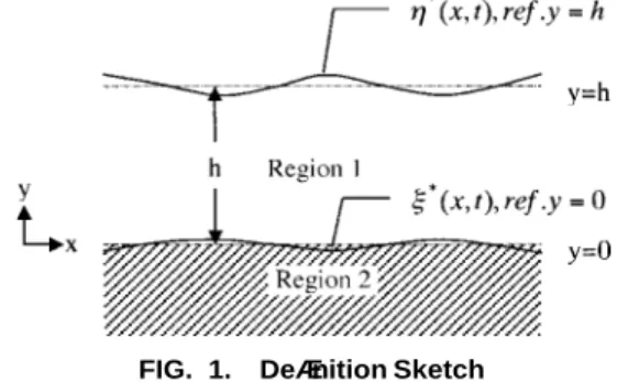
This study on a nonlinear water wave problem is defined in Fig. 1, which indicates that the plane wave propagates over a horizontally infinite thickness and homogeneous poroelastic bed saturated with water. Region 1 is homogeneous water processed as potential flow, and region 2 is a semi-infinite porous medium treated by Biot’s theory of poroelasticity (Biot 1962). The symbols␩* and ␰* in Fig. 1 represent the displace-ments of waves from the mean free surface ( y = h) and mean bed interface ( y = 0), respectively.

(2)

FIG. 1. Definition Sketch

Boundary-Value Problem

Assuming that homogeneous channel flow (region 1 of Fig. 1) is potential flow, the equations of continuity and momentum in terms of velocity potential_⌽*(1)become

2 (1) ⵜ ⌽* = 0 (1) 2 2 (1) (1) (1) ⭸⌽* ␳0 ⭸⌽* ⭸* (1) ␳0 _⭸t ⫹

再冋册冋册冎

⫹ ⫹ P* = 0 (2) 2 ⭸x ⭸y

where (1) = perturbed pressure; and␳0 = water density.

P *

Referring to Huang and Chwang (1990), the linear momen-tum equations of solid skeleton and fluid for the porous bed based on the theory of poroelasticity may be written as

2 2 ⭸ d* ⭸ D* ⭸d* ⭸D* ⵜ⭈␴* = ␳11 _⭸t2 ⫹ ␳12 _⭸t2 ⫹ b

冉

_⭸t ⫺ _⭸t

冊

(3) 2 2 ⭸ d* ⭸ D* ⭸d* ⭸D* ⵜ⭈S* = ␳12 _⭸t2 ⫹ ␳22 _⭸t2 ⫺ b

冉

_⭸t ⫺ _⭸t

冊

(4) with (2) ␴* = ␶* ⫺ (1 ⫺ n )P* I0 (5) ␶* = 2Ge* ⫹ ␭(ⵜ⭈d*)I (6) 1 _t e* = [ⵜd* ⫹ (ⵜd*) ] (7) 2 (2) S* =⫺n P* I0 (8) ␳ = (1 ⫺ n )␳ ⫹ ␳11 0 s a (9) ␳ = ⫺␳12 a (10) ␳ = n ␳ ⫹ ␳22 0 0 a (11) 2 b =␮n /k0 p (12)

where␴* = solid stress tensor, ␶* = effective stress tensor of solid; S* = normal stress tensor of fluid; d* and D* = solid and fluid displacement vectors, respectively; (2) = perturbed

P *

pore pressure inside the porous medium;␳s= solid density;␳a = mass coupling effect (neglected in this study); n0= porosity; ␮ = fluid viscosity; kp = specific permeability; G and ␭ = Lame’s constants of elasticity; I = identity matrix.

Combining continuity equations of solid and fluid with state equation of fluid and after linearization of porosity, one can find

(2)

⭸P* K ⭸d* ⭸D*

=⫺

冋

(1⫺ n )ⵜ⭈0

冉冊冉冊册

⫹ n ⵜ⭈0 (13)

⭸t n0 ⭸t ⭸t

for perturbed pore pressure (2) In (13), K is the bulk

mod-P * .

ulus of compressibility of fluid inside the porous bed. There are three boundaries that require boundary conditions in this study. They are (1) free surface [ y = h⫹ ␩*(x, t)]; (2) channel-bed interface [ y =␰*(x, t)]; and (3) deep far field of the porous bed [ yˆ→⫺⬁].

On the free surface, a kinematic boundary condition exists as

(1) (1)

⭸␩* ⭸⌽* ⭸⌽* ⭸␩*

⫺ ⫹ = (14)

⭸x ⭸x ⭸y ⭸t

and a dynamic boundary condition exists as

2 2

(1) (1) (1)

⭸⌽* 1 ⭸⌽* ⭸⌽*

⫹

再冋册冋册冎

⫹ ⫹ g␩* = 0 (15)

⭸t 2 ⭸x ⭸y

On the porous bed interface, the continuity of pressure gives

(1) (2)

P * = P * (16)

and the conservation of fluid flux gives

⭸d* ⭸D* (1)

* *

n2⭈ (1 ⫺ n )

冋

0 _⭸t ⫹ n0 _⭸t

册

= n2⭈ⵜ⌽* (17) where n*2 = unit normal vector of the porous bed interface. Considering the kinematics of the porous bed interface, one has

⭸␰* ⭸d* ⭸␰*

= ⭈ ⫺

冉冊

, 1 (18)

⭸t ⭸t ⭸x

and (18) will be used to solve␰*. The continuity of effective stresses of solid gives

*

n2⭈␶* = 0 (19)

At the far field of porous bed, y→⫺⬁, the boundary con-ditions are vanishing displacement vectors; that is

d*, D*→0 (20) If 兩␩*兩 and 兩␰*兩 are much smaller than the relative wave-lengths, it is more convenient to shift the boundary conditions at the free surface, y = h ⫹ ␩*(x, t), and the porous bed interface, y = ␰*(x, t), to y = h and y = 0 before solving the boundary-value problem. Conventionally, the Taylor series ex-pansions are applied to the boundary conditions at the free surface [(14) and (15)] and at the porous bed interface [(16), (17), (19), and (18)] by performing, respectively

⬁ m m ⬁ m m (␩*) ⭸ (␰*) ⭸ and

冘

m

冘

m m! ⭸y m! ⭸y m = 0 m = 0

As m = 0, the boundary-wave problem is linear, but as m

ⱖ 1, the problem becomes nonlinear. For nonlinear problems,

the above Taylor series expansions at the interface ( y = 0) are applicable for the first and third kinds of wave but are not applicable for the second kind of wave because there exists a boundary layer that will render errors of the partial derivative in the vertical direction for the second longitudinal wave. That is why Chen et al. (1997) failed to solve the nonlinear problem for soft porous material by only one length scale. To overcome the difficulty, another small parameter, ε2 = k0/k2, other than

ε1= k0a needs to be proposed. Thus, the vertical coordinate y

for the second kind of wave will be enlarged into y⬘ based on this small parameterε2 [see (35b)].

Referring to Huang and Song (1993) for the decoupling processes of Biot’s equations of poroelasticity (Biot 1962), the governing equations (3) and (4) can be rewritten into three decoupled scalar equations as

(2) (2) 2 _* 2 _*

ⵜ ⌽j ⫹ k ⌽j j = 0, j = 1, 2, 3 (21) Also, the perturbed pressure equation [(13)] gives

K (2) (2)

(2) 2 _* 2 _*

P * = [(1⫺ n ⫹ ␣ n )k ⌽0 1 0 1 1 ⫹ (1 ⫺ n ⫹ ␣ n )k ⌽ ]0 2 0 2 2 n0

(3)

where wave numbers kj and solid/fluid related parameters␣j are given as (8) – (20) in Huang and Song (1993). In (21), and are displacement potentials of the first kind and

(2) (2)

* *

⌽1 ⌽2

the second kind of longitudinal waves, respectively, and is the displacement potential of the third kind of

trans-(2)

*

⌽3

verse wave; that is

(2) (2) (2) * * * d* =ⵜ⌽1 ⫹ ⵜ⌽2 ⫹ ⵜˆ(⌽ e )3 Z (23) (2) (2) (2) * * * D* =␣ ⵜ⌽1 1 ⫹ ␣ ⵜ⌽2 2 ⫹ ␣ ⵜˆ(⌽ e )3 3 Z (24) Note that the governing equations (1) and (21) and the pres-sure and effective stresses (2), (22), and (6), together with boundary conditions (14) – (17), (19), and (20), form the com-plete boundary-value problem of the present study.

Nondimensionalized Governing Equations and Boundary Conditions

Huang and Song (1993) defined the following parameters in their solution of a linear water wave propagating over a poroelastic bed: m = (2G⫹ ␭)n /K0 (25) ε= n0␳ ␻/b0 (26) 2 n0␳ ⫹ (1 ⫺ n )␳ ␻0 0 s 2 ⌳ = 2 (27) 2G⫹ ␭ ⫹ (K/n ) k0 0 2 i(m⫹ 1) ␳ ␻0 2 ⌸ = ₂ (28) mε K k0 2 n0␳ ⫹ (1 ⫺ n )␳ ␻0 0 s 2 ⌿ = 2 (29) G k0

in which ε = penetrability parameter; ␻ = frequency; m = stiffness ratio of solid and fluid;⌳ and ⌿ are only functions of water wave speed and material (fluid and solid skeleton) properties, whereas⌸ is not only a function of the same var-iables for ⌳ and ⌿ but also depends on the permeability of porous medium.

For low penetrability (i.e., 储ε储 << 1), (27)–(29) could be simplified to 2 2 ⌳ ⱌ (k /k )1 0 (30) 2 2 ⌸ ⱌ (k /k )2 0 (31) 2 2 ⌿ ⱌ (k /k )3 0 (32)

Moreover, for soft solid skeleton, 储k2储 >> 储k0储 and such that

储⌸2

储 >> 1. Because 储⌳2

储 is always smaller than 储⌿2

储, one can

obtain

2 2 2

储⌳ 储 < 储⌿ 储 << 1 << 储⌸ 储 (33) After the analysis of order of magnitude for each dependent variable, the dimensionless variables are selected as

xˆ = k x0 (34)

yˆ = k y0 (35a)

y⬘ = yˆ/ε2 for the second longitudinal wave only (35b)

ˆt =兹gk t0 (36) ␩ˆ* = k ␩*0 (37) ␻ˆ = ␻/ gk兹 0 (38) 2 k0 (1) (1) ˆ ⌽* = ⌽* (39) gk 兹 0 (2) k h0 2 (2) ˆ * * ⌽1 = e k0⌽1 (40) 2 k h0 2 k2 e k0 (2) k h0 2 (2) (2) * * * ⌽2 = e k0_k2⌽2 = ε2_⌳2 ⌽2 (41) 1 2 (2) k h0 2 (2) * * ⌽3 = e k0⌽3 (42) k h0 k e0 ˆ ␰* = _⌿2 ␰* (43) k0 (1) (1) ˆ ˆ P * = P * (44) ␳ g0 k0 (2) (2) ˆ ˆ P * = P * (45) ␳ g0

All of the symbols of variables on the left-hand side of (34) – (45) are dimensionless, but those on the right-hand side are dimensional. Note that because the vertical length scales need multiple scales, yˆ and y⬘ are proposed for the boundary layer correction approach.

Applying the two-parameter perturbation expansion, veloc-ity potential of channel flow and displacement potentials of the three kinds of wave for the whole domain can be written

(1) 2 2 ˆ ˆ* ˆ* ˆ* ⌽* =ε1␾ ⫹10 ε ε1 2␾ ⫹11 ε1␾ ⫹ O(20 ε ε1 2, . . .) (46) (2) [ j ] [ j ] 2 [ j ] 2 ˆ* ˆ* ˆ ˆ ⌽j =ε1␾10 ⫹ε ε1 2␾*11 ⫹ε1␾20* ⫹ O(ε ε1 2, . . .), j = 1, 3 (47) Due to (33), the second kind of wave needs to be solved inside the boundary layer. The displacement potential of the second kind of wave inside the boundary layer is nondimensionalized specifically as (41) with a magnified length scale [see (35b)] and expanded as

(2) [2] [2] 2 [2] 2

ˆ* ˆ* ˆ* ˆ*

⌽2 =ε1␾10 ⫹ε ε1 2␾11 ⫹ε1␾20 ⫹ O(ε ε1 2, . . .) (48) if储ε2储 and 储ε1储 are smaller than unity. Also, the water wave at the free surface becomes

2 2

* * *

␩ˆ* =ε1␩ˆ ⫹10 ε ε1 2␩ˆ ⫹11 ε1␩ ⫹ O(20 ε ε1 2, . . .) (49) and the wave of the channel-bed interface becomes

2 2

ˆ ˆ_* ˆ_* ˆ_*

␰* =ε1␰ ⫹10 ε ε1 2␰ ⫹11 ε1␰ ⫹ O(20 ε ε1 2, . . .) (50) For a periodic motion with frequency␻, the aforementioned variables [ ]*(R, t) can be written as[ ](R)e⫺i␻t, where R is a position vector. Let the given incoming wave amplitude be-fore being disturbed by the porous bed be a, and if the wave number of this incoming wave is found to be k0 (it will be

found as complex), the Stokes expansion of two parameters based on ε1 andε2 will be carried out only to the first three

terms of the present nonlinear water wave problem to avoid the occurrence of secular terms. Thus, after the Taylor series expansions at the free surface and at the channel-bed interface, respectively, the boundary-value problem of each order, with-out the time factor, is obtained in the following.

Boundary-Value Problem for the First and Third Kinds of Wave O(ε1) Governing equations • Region 1: ⫺⬁ < xˆ < ⬁, 0 < yˆ < k0h 2 ˆ ˆ ⵜ ␾ = 010 (51) • Region 2: ⫺⬁ < xˆ < ⬁, ⫺⬁ < yˆ < 0 2 [3] 2 [3] ˆ ˆ ˆ ⵜ ␾ ⫹ ⌿ ␾ = 010 10 (53) Boundary conditions

(4)

• At the free surface: yˆ = k0h, ⫺⬁ < xˆ < ⬁

(a) Kinematic free surface boundary condition ˆ

␾10, yˆ=⫺i␻ˆ␩ˆ10 (54) (b) Dynamic free surface boundary condition

ˆ

⫺i␻ˆ␾ ⫹ ␩ˆ = 010 10 (55) • At the porous bed interface: yˆ = 0,⫺⬁ < xˆ < ⬁

(a) Continuity of pressure

2 k K0 ⌳ [1] ˆ ˆ ⫺i␻ˆ␾ ⫹10 _ek h0_n ␳ gq1␾ = 010 (56) 0 0 (b) Continuity of flux [3] k h0 [1] ˆ ˆ ˆ q3␾10, xˆ⫹ e ␾10, yˆ= 0 q1␾10, yˆ⫺ i␻ˆ i␻ˆ (57)

(c) Continuity of effective stress (only ␶xyˆ ˆⱌ 0

[1] [3] [3]

ˆ ˆ ˆ

2␾10, xyˆ ˆ⫹ ␾10, yyˆ ˆ⫺ ␾10, xxˆ ˆ= 0 (58) • At the deep far field: yˆ→⫺⬁,⫺⬁ < xˆ < ⬁

[ j ]

ˆ

␾10 →0, j = 1, 3 (59)

where

q = 1j ⫺ n ⫹ ␣ n , j = 1, 30 j 0 (60) Note that only one component of the above boundary condi-tion of continuity of effective stress is needed (i.e.,␶ˆ ˆxyⱌ 0), otherwise it will become overdetermined. (Another condition,

ⱌ 0, includes the effect of the second kind of wave and ␶yyˆ ˆ

will be adopted by the boundary layer correction for the sec-ond kind of wave later.)

O(ε1ε2)

The presentations are identical with those in O(ε1) except

subscripts are changed from 10 to 11.

2 O(ε1) Governing equations • Region 1: ⫺⬁ < xˆ < ⬁, 0 < yˆ < k0h 2 ˆ ˆ ⵜ ␾ = 020 (61) • Region 2: ⫺⬁ < xˆ < ⬁, ⫺⬁ < yˆ < 0 2 ˜k1 2 [1] 2 [1] ˆ ˆ ˆ ⵜ ␾ ⫹20 2⌳ ␾ = 020 (62) k1 2 ˜k3 2 [3] 2 [3] ˆ ˆ ˆ ⵜ ␾ ⫹20 2⌿ ␾ = 020 (63) k3 Boundary conditions

• At the free surface: yˆ = k0h, ⫺⬁ < xˆ < ⬁

(a) Kinematic free surface boundary condition

ˆ ˆ ˆ

␾20, yˆ⫹ 2i␻ˆ␩ˆ = ␩ˆ ␾20 10, xˆ 10, xˆ⫺ ␩ˆ ␾10 10, yyˆ ˆ (64) (b) Dynamic free surface boundary condition

1 ₂ ₂

ˆ ˆ ˆ ˆ

⫺ 2i␻ˆ␾ ⫹ ␩ˆ = i␻ˆ␩ˆ ␾20 20 10 10, yˆ⫺ (␾10, xˆ⫹ ␾ )10, yˆ (65) 2

• At the porous bed interface: yˆ = 0,⫺⬁ < xˆ < ⬁ (a) Continuity of pressure

2 k K0 ⌳ [1] 1 2 2 ˆ _˜ ˆ ˆ ˆ 2i␻ˆ␾ ⫺20 _ek h0_n ␳ gq1␾ = (␾20 ₂ 10, xˆ⫹ ␾ )10, yˆ 0 0 2_ˆ 2 2_ˆ i␻ˆ⌿ ␰10 _ˆ ⌿ k K⌳ ␰0 10 _ˆ[1] ⫺ _ek h0 ␾10, yˆ⫹ _e2k h0 _n␳ g q1␾10, yˆ 0 0 (66) (b) Continuity of flux k h0 ˆ _˜ ˆ[1] _˜ ˆ[3] 2ˆ ˆ e ␾20, yˆ⫹ 2i␻ˆ(q ␾1 20, yˆ⫺ q ␾ ) = ⌿ ␰ ␾3 20, xˆ 10, xˆ 10, xˆ 2ˆ ˆ 2 ⫺k h0 ˆ ˆ[1] ˆ[3] ⫺ ⌿ ␰ ␾10 10, yyˆ ˆ⫹ i␻ˆ⌿ e ␰ (q ␾10, xˆ 1 10, ˆx⫹ q ␾ )3 10, yˆ 2 ⫺k h0 ˆ ˆ[1] ˆ[3] ⫺ i␻ˆ⌿ e ␰ (q ␾10 1 10, yyˆ ˆ⫺ q ␾3 10, yxˆ ˆ) (67) (c) Continuity of effective stress (only␶ˆ ˆxyⱌ 0

[1] [3] [3] ˆ ˆ ˆ G(2␾20, xyˆ ˆ⫹ ␾20, yyˆ ˆ⫺ ␾20, xxˆ ˆ) 2 ⫺k h0 ˆ ˆ[1] ˆ[3] 2ˆ[1] =⌿ e ␰ [2G(␾10, xˆ 10, xxˆ ˆ⫹ ␾10, xyˆ ˆ)⫺ ␭⌳ ␾10 2 ⫺k h0 ˆ ˆ[1] ˆ[3] ˆ[3]

⫺ G⌿ e ␰ (2␾10 10, xyyˆ ˆ ˆ⫹ ␾10, yyyˆ ˆ ˆ⫺ ␾10, xxyˆ ˆ ˆ)] (68) • At the deep far field: yˆ→⫺⬁, ⫺⬁ < xˆ < ⬁

[ j ]

ˆ

␾20 →0, j = 1, 3 (69)

where_k_˜ and_␣_˜ ( j = 1, 3) in nonlinear orderε2 are given

j j 1

as eqs. (8) – (20) in Huang and Song (1993), and

˜ ˜

q = 1j ⫺ n ⫹ ␣ n , j = 1, 30 j 0 (70)

Boundary Layer Correction for Second Kind of Wave

The second kind of wave disappears outside the boundary layer, but it does exist inside the boundary layer; thus the complete solution needs to be corrected by further considering the second kind of wave inside the porous material bed. Be-cause a thin boundary layer exists within the porous bed near the water/porous bed interface, multiple scales are necessary to solve the nonlinear boundary-value problem for the second longitudinal wave. One therefore lets y⬘ = yˆ/ε2 to change the

scale from yˆ to the magnified scale y⬘ in (35b). The difficulty (i.e., the error due to the first partial derivative based on y of the displacement potential of the second longitudinal wave) that Chen et al. (1997) encountered is now overcome by pro-posing this double length scale in the vertical direction. After the coordinate transformation of (35b), the boundary-value problem of the displacement potential of the second longitu-dinal wave inside the boundary layer is as follows.

O(ε1) Governing equations [2] [2] ˆ ˆ ␾10, y⬘y⬘⫹ ␾ = 010 (71) Boundary Conditions: y⬘ = 0, ⫺⬁ < xˆ < ⬁

[2]

ˆ

␾ = 010 (72)

(b) Continuity of effective stress (only␶ˆ ˆyyⱌ 0)

2_ˆ[2] 2_ˆ[2] 2_ˆ[1] _ˆ[1] _ˆ[3]

2G⌳ ␾10, y⬘y⬘⫺ ␭⌳ ␾ = ␭⌳ ␾ ⫺ 2G(␾10 10 10, yyˆ ˆ⫺ ␾10, xyˆ ˆ) (73) Note that the boundary condition of continuity of flux is equiv-alent to (72), and the boundary condition of ␶xyˆ ˆ ⱌ 0 just sat-isfies_␾_ˆ[2] =_⫺␾_ˆ[2] (i.e.,_␾_ˆ[2] = 0). However,_␾_ˆ[2] = 0 at

ˆ ˆ ˆ ˆ

10, xy⬘ 10, y⬘x 10, xy⬘ 10, xy⬘

(5)

FIG. 2. Relation among Solutions of Each Order

one component of the effective stress boundary condition␶yyˆ ˆ

ⱌ 0 is needed to solve_{␾ .}_ˆ[2] 10

O(ε1ε2)

The presentations are identical with those in O(ε1) except

subscripts are changed from 10 to 11.

2 O(ε1) Governing equations [2] [2] ˆ ˆ ␾20, y⬘y⬘⫹ ␾ = 020 (74) Boundary conditions: y⬘ = 0, ⫺⬁ < xˆ < ⬁

2 k K0 ⌳ _˜q_{␾ = 2i␻ˆ␾ ⫺ (␾}_ˆ[2] _ˆ 1 _ˆ[2] _{⫹ ␾ )}_ˆ[2] ˆ ˆ 2 20 20 10, x 10, y k h0 e n0␳ g0 2 2 k K0 ⌳ _˜ ˆ[2] 2ˆ ⫺k h0 ⫺_ek h0_n ␳ gq1␾ ⫺ ⌿ ␰ e20 10 0 0 2 k K0 ⌳ [1] [2] ˆ ˆ ˆ ⭈ ⫺i␻ˆ␾

冋

10, yˆ⫹_ek h0_n ␳ g(q1␾10, yˆ⫹ q ␾2 11, y⬘)

册

0 0 (75)

(b) Continuity of effective stress (only␶yyˆ ˆⱌ 0)

2_ˆ[2] 2_ˆ[2] _ˆ[1] _ˆ[3] 2_ˆ[1]

2G⌳ ␾20, y⬘y⬘⫺ ␭⌳ ␾ = ⫺2G(␾20 20, yyˆ ˆ⫺ ␾20, xyˆ ˆ)⫹ ␭⌳ ␾20 2ˆ ⫺k h0 ˆ[1] 2ˆ[2] ˆ[3]

⫺ ⌿ ␰ e10 [2G(␾20, yyyˆ ˆ ˆ⫹ ⌳ ␾11, y⬘y⬘y⬘⫺ ␾10, xyyˆ ˆ ˆ)

2 _ˆ[1] _ˆ[2]

⫺ ␭⌳ (␾10, yˆ⫹ ␾11, y⬘)] (76)

SOLUTION

After omitting the time factore⫺i␻t,the given incoming wa-ter wave profile with magnitude a is

ik x0

␩ (x) = ae , 0 < x < ⬁10 (77) With the input of the incoming water wave, each order of the aforementioned boundary-value problem can be solved in se-quence as shown in Fig. 2. Fig. 2 indicates that one can first find the solution of order ε1 outside the boundary layer and

can subsequently match it with the inner expansion to com-plete the solution of orderε1. Then, the solution of orderε1is

provided to solve the higher orders in sequence as indicated by the solid arrows as shown in Fig. 2. Note that the problem of order ε1ε2 is solved simultaneously to find the unique

so-lution. Thus the dimensional solutions of the first kind of lon-gitudinal wave and the third kind of transverse wave through-out the entire domain are obtained as follows.

O(ε1) i g ␻ _{ik x} 0 ␾ = ⫺10

冋

cosh k (h0 ⫺ y) ⫺ sinh k (h0 ⫺ y) e

册

(78) k0 ␻ k0 i gk0 [1] K k y1 0⫹ik x0 ˆ ␾ =10 2

冋

cosh(k h)0 ⫺ 2 sinh(k h)0

册

e k (iq K0 1 1⫺ q L )3 1 ␻ (79) a3 [3] K k y3 0⫹ik x0 ˆ ␾ =10 _ek h0_k02e (80) with the dispersion relation of complex wave number k0as

2 T1␻ gk0 T1⫺ 1 =

冉

_gk ⫺ _␻2

冊

tanh(k h)0 (81) 0 where n0␳ g(q K ⫹ iq L )0 1 1 3 1 T =1 2 (82) k K0 ⌳ q1 O(ε1ε2) 2 gk ␻ 兹 0 ik x0 ␾ =11 2 E5

冋

cosh(k y)0 ⫺ sinh(k y)0

册

e (83) k0 gk0 c1 [1] K k y1 0⫹ik x0 ␾ =11 _ek h0 _k02e (84) c3 [3] K k y3 0⫹ik x0 ␾ =11 _ek h0_k2e (85) 0 i ␻ _{ik x} 0 ␩ =11 E e5 (86) k0兹gk0 2 O(ε1) gk 兹 0 2ik x0

␾ =20 2 [E cosh 2k (h3 0 ⫺ y) ⫹ E sinh 2k (h ⫺ y)]e4 0 (87)

k0 b1 [1] M k y1 0⫹2ik x0 ␾ =20 _ek h0_k02e (88) b3 [3] M k y3 0⫹2ik x0 ␾ =20 _ek h0_k2e (89) 0 g iE4 2ik x0 ␩ =20

冉

_␻2⫺_␻k 兹gk0

冊

e (90) 0

The dimensional solutions of the second kind of longitudi-nal wave obtained by the boundary layer correction approach are as follows. O(ε1) 2 a2 k1 y [2] ␾ =10 _{k e}2 k h0 _k2exp ik

TABLE 2. Variables of Very Soft Soil

Notation (1) Value (2) k0 0.245834E⫹01⫹i0.481295E-04 k1 0.238469E-02⫹i0.237891E-07 k2 0.318363E⫹02⫹i0.318331E⫹02 k3 0.808703E⫹00⫹i0.823670E-05 ˜k1 0.476939E-02⫹i0.952280E-07 ˜k2 0.450257E⫹02⫹i0.450166E⫹02 ˜k3 0.161741E⫹01⫹i0.329468E-04 a1 0.127676E⫹01-i0.674232E-03 a2 0.386868E-01-i0.221286E⫹02 a3 ⫺0.714250E-03-i0.134980E⫹01 b1 0.171970E⫹01⫹i0.707839E-03 b2 ⫺0.118767E-03-i0.341805E⫹00 b3 0.749158E-03-i0.181747E⫹01 c1 0.208305E-04-i0.189383E-04 c2 0.110643E⫹02⫹i0.284844E-02 c3 ⫺0.200597E-04-i0.836553E-08

TABLE 1. Material Properties of Very Soft Soil

Item (1) Notation (2) Value (3) Unit (4) (a) Water Density ␳0 1,000 kg/m 3 Bulk modulus K 2.3⫻ 109 N/m2 Dynamic viscosity ␮ 0.001 Ns/m2 Depth h 0.35 m Wave height a 0.0357 m Period T 1.55 s (b) Skeleton Density ␳s 2,650 kg/m 3 Lame’s constant G 5.0⫻ 104 N/m2 Lame’s constant ␭ 1.0⫻ 105 N/m2 Specific permeability kp 1.0⫻ 10⫺11 m 2 Porosity n0 0.4 —

FIG. 3. Schematic Diagram of Two-Parameter Expansion

␻ C gk0 0 ⫺k h ⫺10 _˜ 2k h0 2 2 b = e2 q2

再

2i r C e4 0 ⫺ ₂_␻2 (t1⫺ r )1 gk 兹 0 k h0 _˜ ⫹ (K a ⫺ ia )[C r ⫺ (q a K ⫺ iq c )] ⫺ e q b1 1 3 0 1 1 1 1 2 2 1 1

冎

(96) After solving the displacement potentials, all of the other variables can be obtained. The wave of the porous bed inter-face from (18) gives

ik x0⫺k h0 ik x0⫺k h0 2 ␰(x) = a(K a ⫺ ia )e1 1 3 ⫹ε2ae (c K1 1⫺ ia ⌳ ⫺ ic )2 3 a 2ik x0⫺2k h0 2 2 ⫹ε1 e {(K a1 1⫺ ia )[(K ⫹ 1)a ⫺ a ⌳ ⫺ 2iK a ]3 1 1 2 3 3 2 k h0 k h0 ⫹ 2b M e1 1 ⫺ 4ib e }3 (97)

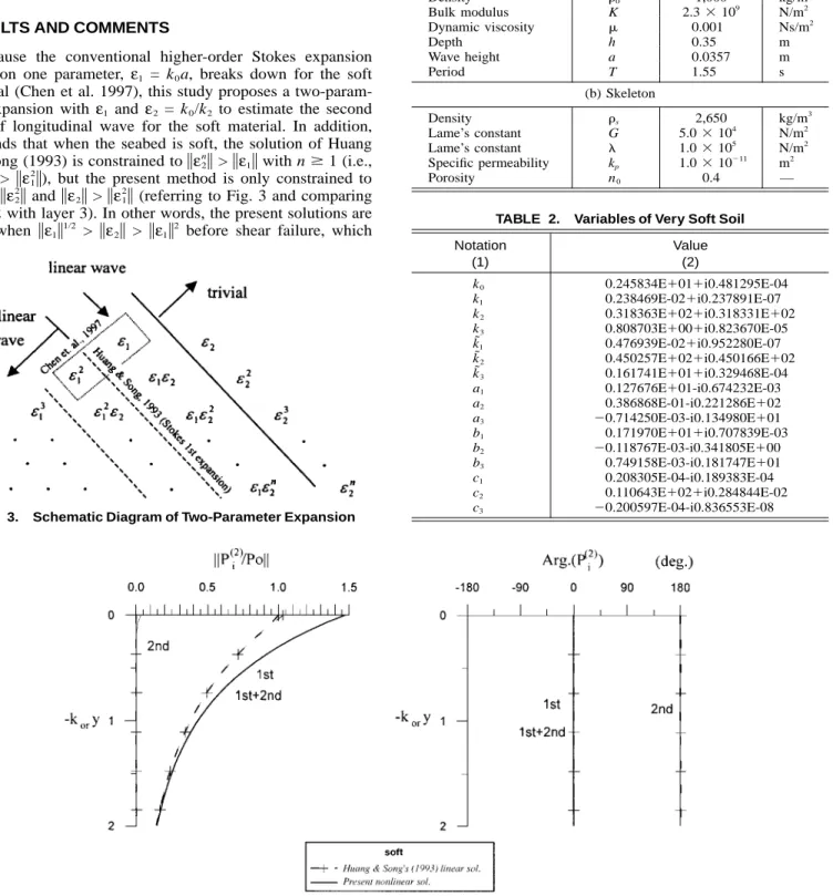
RESULTS AND COMMENTS

Because the conventional higher-order Stokes expansion based on one parameter, ε1 = k0a, breaks down for the soft

material (Chen et al. 1997), this study proposes a two-param-eter expansion with ε1 and ε2 = k0/k2 to estimate the second

kind of longitudinal wave for the soft material. In addition, one finds that when the seabed is soft, the solution of Huang and Song (1993) is constrained to_储εn_储>储ε1储 with n ⱖ 1 (i.e.,

2

> but the present method is only constrained to

n 2

储ε ε2 1储储ε1储),

储ε1储 >_储ε2_储and储ε2储 >_储ε2_储(referring to Fig. 3 and comparing

2 1

layer 2 with layer 3). In other words, the present solutions are valid when 储ε1储

1/2

> 储ε2储 > 储ε1储 2

before shear failure, which

indicates that the present solution is more accurate than the solution of Huang and Song (1993) in the same order of ε2

for soft material. This is indicated clearly in Fig. 3, the sche-matic diagram of the two-parameter expansion. Because the second longitudinal wave decays very quickly in the y-direc-tion near the homogeneous water/porous bed interface, Chen et al. (1997) failed to estimate accurately the first order of partial derivative with respect to y for the displacement poten-tial of the second longitudinal wave inside the boundary layer

(7)

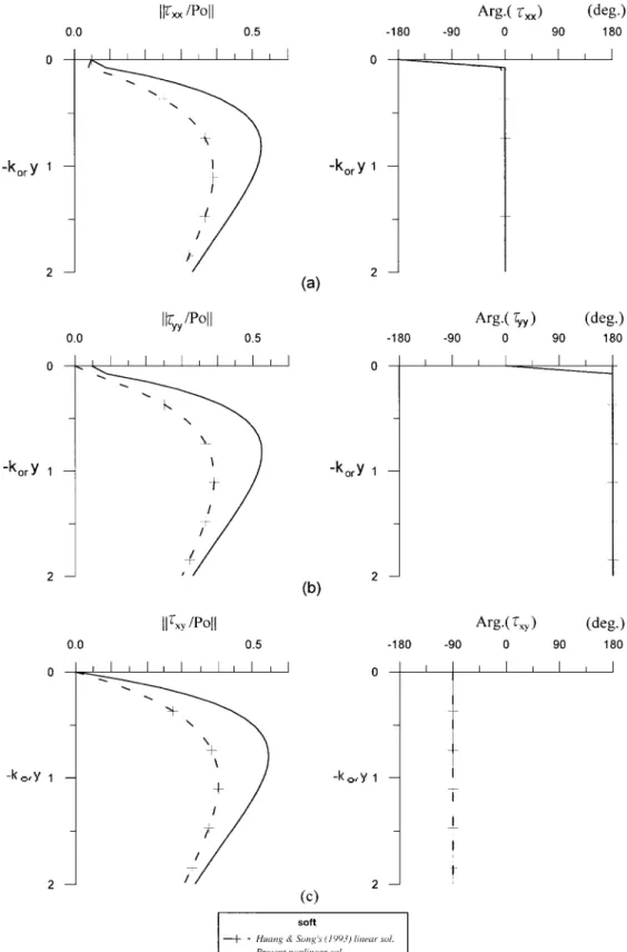
FIG. 5. Variation of Effective Stress for Very Soft Material: (a) xx-component; (b) yy-component; (c) xy-component (储␧1储 ⴝ0.0878,

储␧2储 ⴝ0.0546)

Therefore, one more length scale is needed to estimate

(2)

ˆ_* _.

⌽2

more accurately the first order of partial derivative for ˆ *(2) ⌽2

in the vertical direction by the transformation of y to y⬘ [see (35b)]. Because⌬y⬘ is much shorter than ⌬y, the length scale adopted by Chen et al. (1997) will overestimate the displace-ment potential of the second longitudinal wave. That is why the present method adopts two length scales to reformulate the boundary-value problem inside the boundary layer.

To confirm the validity of the proposed solution, some soft material and wave conditions are selected to compute pore

pressure and effective stresses inside the porous bed as well as the profiles of the channel bed and free surface. The results agree very well to the solutions of Huang and Song (1993). (Because the results are so close to those of Huang and Song’s solutions, the detailed figures will not be shown here to save space.) Because there is good agreement between the present solutions and those of Huang and Song (1993) for the soft porous bed as discussed, one may simply use the present so-lution to show the validity of Biot’s theory of poroelasticity (Biot 1962) in simulating a soft porous bed.

(8)

FIG. 6. (a) Free Surface Profiles; (b) Channel-Bed Interface Profiles of Wave Period 1.55 s with Respect to Time for Very Soft Material (储␧1储 ⴝ0.0878,储␧2储 ⴝ0.0546)

Table 1 shows the material properties of very soft soil, and Table 2 provides the simulation result. Comparing the present Table 2 with Table 2 of Chen et al. (1997), one can find that the unreasonable result — the coefficient of a higher-order term is much larger than that of the leading term (i.e.,兩b2兩 >> 兩a2兩) — does not exist in the present result.

The very soft soil case is illustrated to show the differences between the linear solution of Huang and Song (1993) and the present nonlinear solution, and the simulation results are plot-ted in Figs. 4 – 6. In Fig. 4, P0is the perturbed pressure on bed

at y = 0. In fact, the analytic solution proposed by Huang and Song (1993) failed in this case due to their constrain,_储εn_储 >

2 储ε1储, but the present method is still applicable. Note that the

Ursell number, Ur = Re(k0a)/[Re(k0h)] 3

, is 0.138. Moreover, referring to Fig. 6(a) the water profile is the same as that of Chen et al. (1997) while referring to Fig. 6(b), the soil profile is significantly different than that of Chen et al. (1997). This is because the solution of homogeneous water of Chen et al. (1997) is correct, but the solution of the second longitudinal wave inside the porous medium is wrong. Furthermore, refer-ring to Figs. 7(b – d) of Chen et al. (1997) the experimental data near the peaks and troughs are lower than their nonlinear solution, and the present solution in Fig. 6(b) also has the same tendency as the experimental data [i.e., the present nonlinear solution is lower than that of Chen et al. (1997) in the peaks

and the troughs]. Thus combining Figs. 4 – 6, it can be con-cluded that in simulating a soft porous bed it is proper to adopt a two-parameter expansion instead of the conventional one-parameter expansion.

CONCLUSIONS

When the bed material is soft, the higher-order Stokes ex-pansion of a water wave based on ε1 is invalid [i.e., the

one-parameter perturbation failed (Chen et al. 1997)]. This is be-cause a boundary layer exists inside the porous bed and near the homogeneous water/porous bed interface from the second longitudinal wave. Therefore, considering that the second length scale based on the second longitudinal wave number for the boundary-value problem is necessary, a two-parameter perturbation expansion based on ε1 and ε2 is proposed.

Be-cause the second kind of longitudinal wave vanishes outside the boundary layer, but exists inside the boundary layer, the complete solution of the displacement potential needs to be corrected inside the boundary layer. Hence the complete boundary-value problem is thus solved by the boundary layer correction approach in the present study. Referring to Chen et al. (1997), a nonlinear water wave is very likely to happen even when 储ε1储 and the Ursell parameter are very small, and this is proved again in the present study.

Moreover, due to the effect of the second longitudinal wave inside the soft porous bed, it is very difficult to compute the pore pressure, effective stresses, and bed form accurately near the interface by the numerical model. The numerical model will encounter a problem of convergence even by finding the meshes near the interface. Thus the concept of the present study is very helpful in formulating a simplified boundary-value problem in numerical computation for a soft poroelastic bed with irregular geometry.

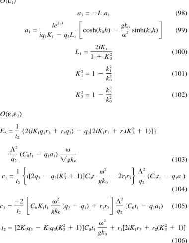
APPENDIX I. COEFFICIENTS OF SOLUTIONS

cosh(2k h)0 2 ␻ gk0兹gk0 (123) f31= 4GM1 (124) 2 f32=⫺iG(M ⫹ 4)3 (125) ⫺k h0 2 f33= e (K a1 1⫺ ia )[2iGa K ⫺ (2G ⫹ ␭⌳ )a ]3 3 3 1 ⫺k h0 2 3 ⫹ e Gi(K a1 1⫺ ia )(2ia K ⫹ a K ⫹ a K )3 1 1 3 3 3 3 (126) 2 ˜k1 2 M = 41 ⫺ 2 (127) k0 2 ˜k3 2 M = 43 ⫺_k2 (128) 0 ACKNOWLEDGMENT

This study is sponsored by National Science Council of the Republic of China under Grant NSC 87-2611-E-002-001.

APPENDIX II. REFERENCES

Biot, M. A. (1962). ‘‘Mechanics of deformation and acoustic propagation in porous media.’’ J. Appl. Phys., 33(4), 1482–1498.

Chen, T. W., Huang, L. H., and Song, C. H. (1997). ‘‘Dynamic response of poroelastic bed to nonlinear water waves.’’ J. Engrg. Mech., ASCE, 123(10), 1041–1049.

Dean, R. G., and Dalrymple, R. A. (1991). Water wave mechanics for

engineers and scientists, World Scientific, Singapore.

Fenton, J. (1985). ‘‘A fifth-order Stokes theory for steady waves.’’ J.

Wtrwy., Port, Coast., and Oc. Engrg., ASCE, 111(2), 216–234.

Huang, L. H., and Chwang, A. T. (1990). ‘‘Trapping and absorption of sound waves. II: A sphere covered with a porous layer.’’ Wave Motion, 12, 401–414.

Huang, L. H., and Song, C. H. (1993). ‘‘Dynamic response of poroelastic bed to water waves.’’ J. Hydr. Engrg., ASCE, 119(9), 1003–1020. Liu, L. F. (1973). ‘‘Damping of water waves over porous bed.’’ J. Hydr.

Div., ASCE, 99(12), 2263–2271.

Madson, O. S. (1978). ‘‘Wave-induced pore pressure and effective stress in a porous bed.’’ Geotech., 28, 377–393.

Mei, C. C. (1983). The applied dynamics of ocean waves, Wiley, New York.

Mei, C. C., and Foda, M. A. (1981). ‘‘Wave-induced responses in a fluid filled poroelastic solid with a free surface—a boundary layer theory.’’

Geophys., 66, 597–631.

Moshagen, H., and Torum, A. (1975). ‘‘Wave induced pressures in per-meable seabeds.’’ J. Wtrwy., Harb. and Coast. Engrg. Div., ASCE, 101(1), 49–57.

Putnam, J. A. (1949). ‘‘Loss of wave energy due to percolation in a permeable sea-bottom.’’ Trans. Am. Geophys. Union, 30, 349–356. Reid, R. O., and Kajiura, K. (1957). ‘‘On the damping of gravity waves

over a permeable sea bed.’’ Trans. Am. Geophys. Union, 30, 662–666. Sleath, J. F. A. (1970). ‘‘Wave induced pressure in bed of sand.’’ J. Hydr.

Div., ASCE, 96, 367–378.

Yamamoto, T., Koning, H. L., Sellmeijer, H., and Hijum, E. V. (1978). ‘‘On the response of a porous-elastic bed to water waves.’’ J. Fluid

Mech., Cambridge, U.K., 87, 193–206.

APPENDIX III. NOTATION

The following symbols are used in this paper:

a = amplitude of incoming water wave;

D* = displacement vector of fluid in porous medium; d* = displacement vector of solid skeleton;

G,␭ = Lame’s constants of elasticity; h = mean water depth of channel;

i = _兹⫺1;

K = bulk modulus of compressibility of fluid; kj = wave numbers in porous medium, j = 1, 2, 3;

kp = specific permeability;

k0 = wave number of incoming water wave;

n0 = porosity; (1)

P * = perturbed pressure in channel;

(2)

P * = perturbed pressure in porous medium;

P0 = perturbed pressure on bed;

(10)

ε1 = first expansion parameters of Stokes wave, k0a;

ε2 = second expansion parameters of Stokes wave, k0/k2; ␩* = displacement of wave deviated from mean free

sur-face;

⌳, ⌸, ⌿ = Mach numbers of two longitudinal waves and one transverse wave;

␮ = dynamic viscosity of fluid;

␰* = displacement of wave deviated from mean channel-bed interface;

␳s = density of solid;

␳0 = density of water; ␴* = solid stress tensor;

␶* = effective solid stress tensor; (1)

*

⌽ = velocity potential of channel flow;

(2)

*

⌽j = jth kind of displacement potentials of porous me-dium, j = 1, 2, 3; and

␻, ⍀ = angular frequencies of water wave, in O(ε1) and O(ε1ε2),⍀ = ␻; in ⍀ = 2␻.

2 O(ε1),

Dynamic response of soft poroelastic bed to nonlinear water waves — a boundary layer correction approach

D

YNAMIC

R

ESPONSE OF

S

OFT

P

OROELASTIC

B

ED TO

N

ONLINEAR

W

ATER

W

AVE

—B

OUNDARY

L

AYER

C

ORRECTION

A

PPROACH

By P. C. Hsieh,

L. H. Huang,

Associate Member, ASCE, and T. W. Wang

再冋 册 冋 册冎

冉

冊

冉

冊

冋

冉 冊 冉 冊册

再冋 册 冋 册冎

冋

册

冉 冊

冘

冘

冋

册

冋

册

冋

册

冉

冊

冋

册

冉

冊

冋 冉 冊册

冋 冉 冊册

冉

冊冒

冋 冉 冊册

再

冎

冋

册

再

冎

冋

册

冋

册

冋

册

冋

冉

冊册

冋

册

冉

冊

冋

册

冉 冊

再冋册冋册冎

冉冊冉冊册

再冋册冋册冎

冉冊

冋冉冊册

冋冉冊册

冋冉冊册

冉冊