以低狀態機率切換與可調變擷取長度為基礎之維特比解碼器

國立交通大學

電子工程學系 電子研究所碩士班

碩 士 論 文

以低狀態切換機率與可調變擷取長度為基礎之低功率

維特比解碼器

A Low-power Viterbi Decoder Based on Scarce State

Transition and Variable Truncation Length

學生 ： 林 大 嘉

指導教授 ：李鎮宜 教授

以低狀態切換機率與可調變擷取長度為基礎之低功率

維特比解碼器

A Low-power Viterbi Decoder Based on Scarce State

Transition and Variable Truncation Length

研 究 生：林大嘉 Student：Dah-Jia Lin

指導教授：李鎮宜 Advisor：Chen-Yi Lee

國 立 交 通 大 學

電子工程學系 電子研究所 碩士班

碩 士 論 文

Submitted to Department of Electronics Engineering & Institute of Electronics College of Electrical and Computer Engineering

National Chiao Tung University in Partial Fulfillment of the Requirements

for the Degree of Master of Science

in

Electronics Engineering July 2007

Hsinchu, Taiwan, Republic of China

以低狀態切換機率與可調變擷取長度為基礎之低功率

維特比解碼器

學生：林大嘉 指導教授：李鎮宜 教授

國立交通大學

電子工程學系 電子研究所碩士班

摘要

A Low-power Viterbi Decoder Based on Scarce State

Transition and Variable Truncation Length

Student：Dah-Jia Lin Advisor：Dr. Chen-Yi Lee

Department of Electronics Engineering

Institute of Electronics

National Chiao Tung University

ABSTRACT

As wireless and portable devices become more and more popular these years, low-power design has become an important issue. In this thesis, we propose a low-power Viterbi decoder combining scarce state transition and variable truncation length schemes. The SST technique reduces the state transition activity significantly in high SNR conditions. The variable truncation scheme eliminates unnecessary data movement of the survivor memory based on path merging property of Viterbi algorithm. According to the simulation results, more than 14% decoder power and 53% survivor memory power can be reduced as Eb/N0 is large than 4dB, while the

誌 謝

Contents

Chapter 1 Introduction...

1.1 Overview of Channel Coding...1

1.2 Research Motivation...3

1.3 Organization of the Thesis ...3

Chapter 2 Convolutional Code and Viterbi Algorithm...

2.1 Convolutional Code ...4

2.1.1 Encoding of Convolutional code ...4

2.1.2 Trellis Diagram of Convolutional Code ...7

2.2 Viterbi Algorithm...9

2.2.1 Maximum Likelihood Decoding ...9

2.2.2 Viterbi Decoding Algorithm ...11

2.2.3 Path Merging Property...14

Chapter 3 Architecture of Viterbi Decoder ...

3.1 Branch Metric Unit...17

3.2 Add-Compare-Select Unit ...19

3.2.1 Radix-2 ACS Structure ...19

3.2.2 High-radix ACS and Two-dimension ACS...20

3.3 Path Metric Unit ...24

3.4 Survivor Memory Unit ...26

3.4.2 Trace-back Approach...31

Chapter 4 Some low-Power Schemes for Viterbi Decoder...

4.1 Scarce-State-Transition (SST) Algorithm ...37

4.2 Adative Viterbi Algorithm...42

4.3 Variable Truncation Length...43

Chapter 5 The Proposed Low-power Viterbi Decoder...

5.1 The Design of Proposed Viterbi Decoder...48

5.1.1 Implementation of SST...49

5.1.2 Radix-2x2 ACS Structure ...50

5.1.3 Implementation of Variable Truncation Length ...53

5.2 Simulation and Implementation Results...55

5.3 Comparison ...62

Chapter 6 Conclusion and Future work ...

List of Figures

Figure 1.1 Block diagram of a digital communication system...1

Figure 2.1 The (2, 1, 2) convolutional encoder ...5

Figure 2.2 State diagram of the convolutional encoder in Figure 2.1 ...8

Figure 2.3 The trellis diagram of the convolutional encoder in Figure 2.1...9

Figure 2.4 The system blocks that focuses on the channel coding...10

Figure 2.5 Viterbi decoding over an ideal channel...13

Figure 2.6 Viterbi decoding over a noisy channel ...14

Figure 2.7 Path merging phenomenon ...15

Figure 2.8 Truncated survivor paths...15

Figure 3.1 Main blocks of Viterbi decoder ...16

Figure 3.2 Quantization of the received symbol...17

Figure 3.3 The architectures of branch metric unit...18

Figure 3.4 The 4-state radix-2 trellis and the radix-2 ACS unit for state S0...20

Figure 3.5 The 4-state radix-2 and radix-4 trellis diagrams ...21

Figure 3.6 A radix-4 ACS unit...21

Figure 3.7 The 4-way comparator in Figure 3.6...22

Figure 3.8 The 4-state radix-2 and radix-2×2 trellis diagrams ...23

Figure 3.10 Circular representation of the modular theorem...25

Figure 3.11 The upper bound of path metric difference...26

Figure 3.12 The best state approach with truncation length 4 ...28

Figure 3.13 Realization of the best state approach ...28

Figure 3.14 The fixed state approach with truncation length 4...29

Figure 3.15 Realization of the fixed state approach...29

Figure 3.16 The majority vote approach with truncation length 4 ...30

Figure 3.17 Realization of the majority vote approach ...30

Figure 3.18 Memory structure and operation of the 3-pointer odd approach ...33

Figure 3.19 Memory structure and operation of the 3-pointer even approach...34

Figure 3.20 Memory structure and operation of the one-pointer approach ...35

Figure 3.21 Memory structure and operation of the even hybrid approach...36

Figure 4.1 The block diagram of convolutional code...38

Figure 4.2 The model of SST Viterbi decoding...38

Figure 4.3 The SST Viterbi decoding process...40

Figure 4.4 The survivor paths over a noiseless channel ...41

Figure 4.5 The ACS unit of adaptive Viterbi decoder ...43

Figure 4.6 A 64-state, radix-2x2 Viterbi decoder with RE-based memory ...44

Figure 4.7 A RE-based survivor memory with variable truncation length ...45

Figure 4.8 Trellis diagram representation of variable truncation length ...46

Figure 5.1 The block diagram of MB-OFDM UWB system ...48

Figure 5.3 The convolutional encoder of MB-OFDM UWB system...49

Figure 5.4 The pre-decoder for the convolutional encoder in Figure 5.3...50

Figure 5.5 The 4-state radix-4 and radix-2x2 trellis diagrams ...51

Figure 5.6 The radix-4 and radix-2x2 ACS units ...51

Figure 5.7 The implementation of variable truncation length...54

Figure 5.8 The performance curves under different truncation lengths ...55

Figure 5.9 The performance curves under different verification conditions ...56

Figure 5.10 The power simulation results in different channel conditions...58

Figure 5.11 The gate count distribution of conventional and proposed designs ...59

Figure 5.12 The power profiling of conventional and proposed designs...60

List of Tables

Table 3.1 Comparison of different radix-2τ

ACS structures ...22

Table 5.1 Comparison of complexity between radix-4 and radix-2×2 ACS units ...52

Table 5.2 The gate counts of different comparators and multiplexers...52

Table 5.3 Design parameters of the proposed Viterbi decoder ...57

Table 5.5 The chip summary...61

Chapter 1

Introduction

1.1 Overview of Channel Coding

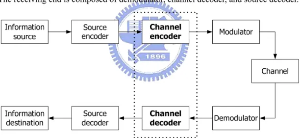
A communication system connects an information source to a destination through a channel. The physical channel may be wireline cables, microwave links, and even storage media. Figure 1.1 shows a typical digital communication system. The transmission end is composed of source encoder, channel encoder, and modulator. The receiving end is composed of demodulator, channel decoder, and source decoder.

Figure 1.1 Block diagram of a digital communication system

A signal will be distorted by some effects such as noise, interference, and fading as it passes through the channel. To overcome the channel effects, the channel

encoder introduces some redundancy in the output of the source encoder, called the information sequence. Next, the modulator converts the new sequence with

redundancy, called the codeword sequence, into analog signals transmitted through the channel. In the receiver, the demodulator estimates the transmitted signal and

makes some error because of channel noise. The demodulated sequence is called

received sequence, which may not match the codeword sequence due to the errors.

The channel decoder uses the redundancy in the codeword to correct the errors in the received sequence and produces an estimate of the information sequence. A subject dealing with the design of channel encoder and channel decoder, referred to channel

coding or error control coding, are developed to improve the performance of the

overall system.

There are two main types of channel coding, the block code and the convolutional code. For the block codes, the encoder transforms a block of k information symbols into a block of n symbols called a codeword. These codes are usually referred as (n, k) block codes. The (n-k) redundancy symbols, also termed as parity symbols, depend only on the corresponding k information symbols and not on other information symbols. This means the block code is memoryless. Some of the commonly used block codes are Hammimg code, BCH code, Reed-Solomon (RS) code, and low-density parity-check (LDPC) code.

For the Convolutional code, the encoder contains memory elements. The (n, k, m) Convolutional encoder has k inputs, n outputs, and m memory elements. Convolutional code converts the entire data stream into one single codeword by a linear shift-register circuit that performs a convolutional operation on the information sequence. The encoded bits depend not only on the current k input bits but also on the previous bits.

The Viterbi algorithm [1] proposed by A.J. Viterbi in 1967 is used to decode convolutional code. Forney [2] later proves that the Viterbi algorithm provides a maximum likelihood (ML) decoding algorithm. Until now, Viterbi algorithm is still the optimal solution for convolutional code and has become an important algorithm in communication systems.

1.2 Research Motivation

In the early research of the Viterbi decoder, low complexity and high throughout are two important concerns in VLSI design. As modern communication systems are required to transmit information at high data rates, the power dissipation has also become an important issue. Nowadays, mobile and wireless system applications are more and more popular. Therefore, a low power design is the key point of the overall system.

Convolutional code is a common error control code in practical communication system. The Viterbi decoder consumes much power in the receiver because of the computing complexity. Therefore, applying low-power techniques to the Viterbi decoder will effectively reduce the power consumption of the whole system. In this thesis, we propose a low-power Viterbi decoder for wireless communication systems.

1.3 Organization of the Thesis

This thesis is organized as follows. In chapter 2, we describe the fundamentals of convolutional code and Viterbi algorithm. The general architectures of Viterbi decoder will be introduced in chapter 3. In chapter 4, some low-power schemes for Viterbi decoder will be presented. In chapter 5, we proposed a low-power Viterbi decoder with reduced state transition and efficient memory access. The implementation results and some comparison will also be presented. Finally, the conclusions and future work are given in chapter 6.

Chapter 2

Convolutional Code and Viterbi

Algorithm

2.1 Convolutional Code

Convolutional code is a widely used error control code in modern communication systems such as DVB-T, IEEE 802.11, IEEE 802.16, and MB-OFDM UWB systems. To describe a convolutional code, one needs to characterize the encoding process. Several methods such as matrix and polynomial representation are used for representing the encoding process of convolutional code. In addition, the trellis diagram description is a common way for illustrating the codeword sequence with timing information. All of them will be introduced in this section.

2.1.1 Encoding of Convolutional Code

A convolutional encoder generates a coded output data stream from an input data stream. As mentioned in previous chapter, a convolutional code is specified in (n, k, m) format where (n, k, m) denotes the number of output, the number of input, and the number of memory element respectively. The coding rate is k/n which means k input bits produce n output bits. The coded bit depends not only on the current input bit but also on m previous input bits. A convolutional encoder is composed of several shift registers and modulo-2 adders (or the XOR operation). Figure 2.1 shows a (2, 1, 2) convolutional encoder with two shift registers and three modulo-2 adders. It produces 2-bit encoded codeword for 1-bit input information.

(2) (2) (2) 2 1 0

c c c

…

c c c

…

u u u

…

Figure 2.1 The (2, 1, 2) convolutional encoder

The input of this encoder is some binary sequence, u=( , , , )u u u_{0 1 2} … . The output is an interleaved sequence of the two binary sequences and . For each input bit, the coded symbol and are generated by the following function

(1) (2) (1) (2) (1) (2) 0 0 1 1 2 2 ( , , , , , , c= c c c c c c …) 2 (1) c _c(2) (1) i c (2) i c (1) 1 i i i i c = ⊕u u₋ ⊕u₋ (2.1) (2) 2 i i i c = ⊕u u₋ (2.2)

where denotes the XOR operation. Next, the input bit is shifted into the leftmost register and the bits in the registers are shifted one position to the right. Therefore, the codeword sequence c depends on not only the current input bit but also on the two previous input bits and

⊕

i u 1

i

u₋ u_i−2. Obviously, the interconnection of the encoder influences the codeword sequence. In general, these interconnections of a (n, k, m) convolutional encoder can be formulized as the generator sequences

(2.3) (1) (1) (1) (1) 0 1 (2) (2) (2) (2) 0 1 ( ) ( ) ( ) ( ) 0 1 ( , , , ) ( , , , ( , , , m m n n n n m g g g g g g g g g g g g ⎧ = ⎪ ₌ ⎪ ⎨ ⎪ ⎪ ₌ ⎩ … … … ) ) )

where represents the interconnections for coded symbol from left to right.

( ) ( ) ( ) 0 1

( i , i , , i m

For information sequence u, the encoding process can be represented in a matrix form as

c uG= (2.4)

where G is called the generator matrix. For a (n, k, m) convolutional code, the generator matrix is made up in the form of

(1) (2) ( ) (1) (2) ( ) (1) (2) ( ) (1) (2) ( ) 0 0 0 1 1 1 2 2 2 (1) (2) ( ) (1) (2) ( ) (1) (2) ( ) 0 0 0 1 1 1 n n n n m m m n n m m m g g g g g g g g g g g g g g g g g g g g g ⎡ ⎤ ⎢ ⎥ ⎢ ⎥ ⎢ ⎥ ⎢ ⎥ ⎢ ⎥ ⎢ ⎥ ⎣ ⎦ … … … … … … … … … … … … n

where each row of the matrix is obtained by interleaving the generator sequences. For example, the (2, 1, 2) convolutional encoder in Figure 2.1 can be described by

(2.5) (1) ₍₁₁₁₎ g = (2.6) (2) ₍₁₀₁₎ g =

Assume the input information sequence is 1011100

u= … (2.7)

Then the coded sequence can be analyzed as 1 1 1 1 0 1 1 0 1 1 1 0 1 1 1 1 1 1 0 1 1 1 1 1 1 0 1 1 1 1 1 1 0 1 1 0 1 1 1 0 1 0 1 1 T c ⎡ ⎤ ⎡ ⎤ ⎢ ⎥ ⎢ ⎥ ⎢ ⎥ ⎢ ⎥ ⎢ ⎥ ⎢ ⎥ ⎢ ⎥ ⎢ ⎥ ⎢ ⎥ ⎢ ⎥ = ⎢ ⎥ ⎢ ⎥ ⎢ ⎥ ⎢ ⎥ ⎢ ⎥ ⎢ ⎥ ⎢ ⎥ ⎢ ⎥ ⎢ ⎥ ⎢ ⎥ ⎢ ⎥ ⎢ ⎥ ⎣ ⎦ ⎣ … … … … …⎦ 1 1 0 1 1 (2.8)

Finally, the interleaved codeword sequence can be obtained as

(2.9)

11,10, 00, 01,10, 01,11,

c= …

In addition to the matrix representation, the encoding process can be described in a polynomial form. A (n, k, m) convolutional encoder is often characterized by the

generator polynomial. The degree of the generator polynomial is less or equal than m.

The coefficient of each term is either 1 or 0, depending on whether a connection exists between the shift register and the modulo-2 adder. For example, the generator polynomial of the (2, 1, 2) convolutional encoder in Figure 2.1 can be written as

(1)_{( ) 1} 2

g D = + +D D (2.10)

(2)_{( ) 1} 2

g D = +D (2.11)

where the factor D means the unit delay operation. For information polynomial u(D), the encoded polynomials are expressed by

(2.12) (1)_{( ) ( )} (1)_{( )} c D =u D g D (2.13) (2)_{( ) ( )} (2)_{( )} c D =u D g D

Assume the information sequence is the same as that of previous example, the input polynomial can be represented as

2 3

( ) 1

u D _{= +}D ₊D ₊D4 _(2.14)

Then the encoded the encoded polynomials become

(2.15) (1)_{( ) (1} 2 3 4₎₍₁ 2_{) 1} 4 c D = +D +D +D + +D D = + +D D +D6 6 (2)_{( ) (1} 2 3 4₎₍₁ 2_{) 1} 3 5 c D = +D +D +D +D = +D +D +D (2.16) Thus the interleaved codeword sequence is

(2.17)

11,10, 00, 01,10, 01,11,

c= …

which agree with the result from previous example.

2.1.2 Trellis Diagram of convolutional code

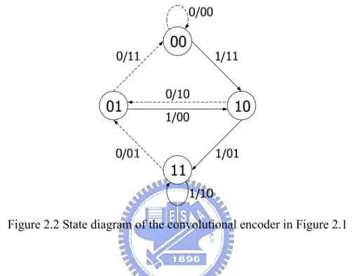
One can regard a convolutional encoder as a finite state machine, where the output is a function of the current input and the current state. Thus, the operation of a convolutional encoder can be specified by the state diagram. Figure 2.2 shows the state diagram of the convolutional encoder in Figure 2.1. As there are two shift registers in the encoder circuit, the contents of these shift registers will have four

states represented as 00, 01, 10, and 11. A state transition corresponding to an information bit “0” is represented by a dotted line. Similarly, a state transition corresponding to an information bit “1” is represented by a solid line. The label on the line represents the information input and the corresponding codeword symbols generated by the state transition.

Figure 2.2 State diagram of the convolutional encoder in Figure 2.1

With the state diagram, it is easy to determine the codeword sequence in the encoding process. For example, assume the information sequence is (1011100…). The transition starts at state 00 and goes through the state diagram corresponding to a solid line if the information bit is “1”, and a dotted line if that is “0”. Following the track, the codeword sequence is (11, 10, 00, 01, 10, 01, 11,…). This codeword sequence is the same as the result described in section 2.1.1.

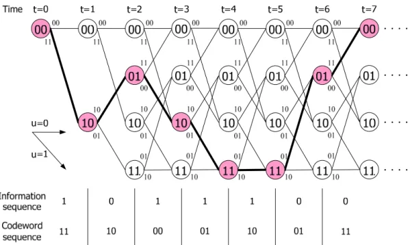
As the length of information sequence is large, it is difficult to trace the codeword sequence from the state diagram. Therefore, a representation called a trellis diagram is obtained from an extension of the state diagram that shows the dimension of time. Figure 2.3 shows encoding process for the information sequence (1011100…) by the trellis diagram. With the trellis diagram, it is easy to illustrate the encoding process as well as the decoding process described in next section.

Figure 2.3 The trellis diagram of the convolutional encoder in Figure 2.1

2.2 Viterbi Algorithm

The Viterbi algorithm [1] proposed by A.J. Viterbi in 1967 is used to decode convolutional code. Forney [2] later proves that the Viterbi algorithm provides a maximum likelihood (ML) decoding algorithm. In fact, an optimum solution to decode a convolutional code is equivalent to find the maximum likelihood path in the trellis diagram. Until now, Viterbi algorithm is still the optimal solution for convolutional code and has become an important algorithm in communication systems. The maximum likelihood decoding and Viterbi algorithm will be introduced in this section.

2.2.1 Maximum Likelihood Decoding

Figure 2.4 shows a simplified communication system that focuses on the channel coding. The encoder transforms the information sequence u into the codeword sequence c by adding certain structural redundancy. Then the codeword sequence c is

transmitted across the noisy channel. The decoder uses the redundancy to correct the errors in the received sequence r and produces an estimate which is the most possible information sequence.

ˆu

u

c

r

ˆu

Figure 2.4 The system blocks that focuses on the channel coding

The maximum likelihood decoder finds the sequence that maximizes the probability . Considering a rate k/n convolutional code, assume the information sequence u is composed of L k-bit blocks.

ˆc ( | ) P r c (0) (1) ( 1) (0) (1) ( 1) ( 1) 0 0 0 1 1 1 1 ( , , , k , , , , k , , L u= u u … u − u u … u − … uk₋− ) n− n− n− )

The codeword sequence c generated by the convolutional encoder consists of L n-bit

blocks. (0) (1) ( 1) (0) (1) ( 1) ( 1) 0 0 0 1 1 1 1 ( , , , n , , , , n , , ) L c= c c … c − c c … c − … c ₋

The decoder receives sequence r and generates the maximum likelihood sequence . They have the following form.

ˆc (0) (1) ( 1) (0) (1) ( 1) ( 1) 0 0 0 1 1 1 1 ( , , , n , , , , n , , ) L r= r r … r − r r … r − … r₋ (0) (1) ( 1) (0) (1) ( 1) ( 1) 0 0 0 1 1 1 1 ˆ (ˆ ,ˆ , ,ˆn ,ˆ ,ˆ , ,ˆn , ,ˆ ) L c= c c … c − c c … c − … c ₋

The probability can be expressed as

(2.18)

( )

∏

∏ ∏

1 1 ( ) ( ) 0 0 ( | ) ˆ arg max ( | ) arg max L n j j i i i j c c c P r c P r c − − = = = ⎡ ⎤ ⎢ ⎥ ⎣ ⎦ =

∏ ∏

Taking the logarithm conversion to equation (2.19), the product terms turn into summation terms. Thus, the estimation becomes ˆc

(

)

ˆ arg max log ( | )

arg max log ( | ) ( | ) ( | ) arg max log ( | )

1 arg max log exp

2 2 c L n n i i i i i i c _i L n j j i i c _{i j} j j n i i c i j c P r c P r c P r c P r c P r c r c σ πσ − − − = − − = = − = = = ⎡ ⎤ = _{⎣ ⎦} ⎡ ⎤ = _{⎢ ⎥} ⎣ ⎦ ⎡ ⎡ ₋ ⎤⎤ ⎢ ⎢ ⎥ = − ⎢ ⎢ ⎥⎥ ⎣ ⎦ ⎣ ⎦

∏

∑ ∑

∑

(

)

(

)

2 2 arg min L j j L n i i c i j L n j j i i c i j r c r c σ πσ − − − = = − − = = ⎡ ⎡ ₋ ⎤⎤ ⎢ ⎢ ⎥⎥ = − ⎢ ⎢ ⎥⎥ ⎣ ⎦ ⎣ ⎦ ⎡ ⎤ = _⎢ − _⎥ ⎣ ⎦

∑

∑ ∑

∑ ∑

Equation (2.20) shows that to maximize is equivalent to minimize Euclidean distance of and . This rule is also the function of Viterbi algorithm which will be described in next subsection.

log ( | )P r c

r c

2.2.2 Viterbi Decoding Algorithm

The goal of Viterbi algorithm is to find codeword that maximize the probability . According to the maximum likelihood decoding rule, Viterbi proposed an algorithm to compute the minimum Euclidean distance as time goes on. There are two basic measures defined in the Viterbi algorithm, which are branch metric

( | ) P r c x y t s s BM _→

and path metric

y

t s

PM . At each time t, the branch metric and path metric are

x y t s s (2.21)

(

)

(

)

∑

The branch metric is the Euclidean distance between a received symbol and the corresponding trellis codeword symbol.

x y

t s s

BM _→ represents the branch metric associated with the transition between the state s at time t-1 and state _x sy at time t.

The path metric is the minimum Euclidean distance between a received sequence and the corresponding trellis codeword sequence.

y

t s

PM represents the path metric of the

state s_y at time t. In other words, the path metric is the accumulation of branch metrics that across the corresponding paths. Therefore, the Viterbi algorithm can find the minimum path metric at each time instant. Then the maximum likelihood sequence can be estimated in trellis diagram along the minimum path metric.

For a (n, k, m) convolutional code, the steps of the Viterbi algorithm can be described as the following.

z Step 1.

Initially, set path metrics as

0 0 0 0

0 0, 1 2 2m 1

PM = PM =PM =…=PM ₋ = ∞ z Step 2.

Increase time index by 1.For each {0,1, , 2m 1}

y

S ∈ … − , update path metrics as

1 ,

min | {all states merged into }

y x x y

t t t

s s s s x

PM = ⎡_⎣PM − +BM _→ S ∈ S_y ⎤_⎦

and store the survivor at time t. The survivor means the decision bit corresponding to the chosen branch from all branch merged into S_y.

z Step 3.

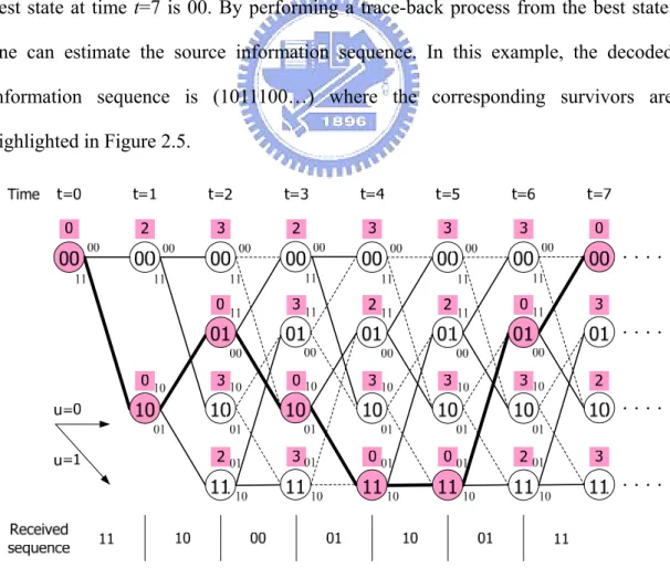
Figure 2.5 illustrates the Viterbi decoding process over an ideal channel by the trellis diagram. Assume the information sequence is the same as the example described in Figure 2.3, the codeword sequence (11, 10, 00, 01, 10, 01, 11,…) is transmitted through the channel. Based on the assumption of ideal channel, the received sequence will be the same as the codeword sequence. The path metric is labeled above each state. As previous mentioned, the path metric of state 00 at time

t=0 is initialized to 0. At each time instant, the path metric is updated and only one of

branches merged to the current state is preserved. The preserved branches, called the survivors, are represented by solid lines. On the other hand, the discarded branches are represented by dotted lines. When the computation of survivors and path metrics are done, the next step is to decode the information sequence . In Figure 2.5, the best state at time t=7 is 00. By performing a trace-back process from the best state, one can estimate the source information sequence. In this example, the decoded information sequence is (1011100…) where the corresponding survivors are highlighted in Figure 2.5.

ˆu

As the codeword sequence is transmitted through a noisy channel, the received sequence may not match the original codeword sequence due to the channel noise. Figure 2.6 shows the Viterbi decoding process over a noisy channel. Considering the same codeword sequence as that of previous example is transmitted through the channel, assume the received sequence including two-bit errors is (11, 11, 00, 01, 10, 00, 11,…) . In Figure 2.6, the errors are represented in boldface. By the process mentioned before, one can obtain the decoded information sequence (1011100…) which is identical to the source information bits.

Figure 2.6 Viterbi decoding over a noisy channel

2.2.3 Path Merging Property

Figure 2.7 shows the survivors in Figure 2.6 and four survivor paths corresponding to each state. Figure 2.7 also shows the path merging property of the Viterbi algorithm. In this example, all survivor paths will merge to the survivor path with the minimum path metric after the merged point. In other words, the decoded data is determined after all survivor paths merge, whether the trace-back operation starts from the best state or not.

Figure 2.7 Path merging phenomenon in Figure 2.6

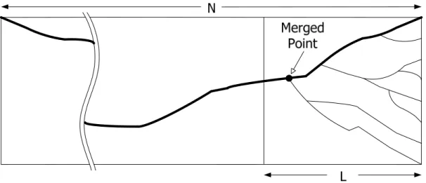
The path merging property of the Viterbi algorithm is an important characteristic for hardware implementation. In practical application, the length of the information sequence may be very large. To reduce the storage requirement and the decoding latency, the survivor path should be truncated to a finite length, called the truncation length. Figure 2.8 shows the truncated survivor paths while the length of information sequence is N. The boldface line means the survivor path with minimum path metric. All survivor paths will merge with high probability if the truncation length L is long enough. By selecting proper truncation length, the decoded data can be determined with L-stage information only. Moreover, it is unnecessary to search for the best state.

Chapter 3

Architecture of Viterbi Decoder

In this chapter, we will introduce the hardware implementation of the Viterbe algorithm. Figure 3.1 shows the main blocks of Viterbi decoder. A Viterbi decoder is usually composed of four basic units. They are summarized as following.

z Branch Metric Unit (BM Unit):

According to the received sequence, compute the branch metric for different branches in trellis diagram.

z Add-Compare-Select Unit (ACS Unit):

Accumulate the branch metric recursively and perform comparison operation to generate the path metric for each state. Decide the survivor corresponding to each state according to the comparison result.

z Path Metric Unit (PM Unit):

Store the path metric at each time instant. z Survivor Memory:

Store the survivors from ACS unit. Then use the register-exchange approach or trace-back approach to decode the maximum likelihood information sequence.

3.1 Branch Metric Unit

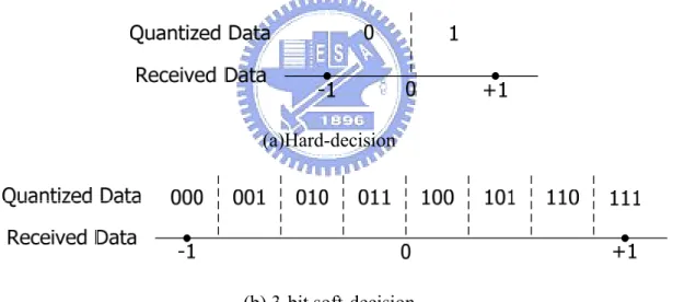
This unit generates all branch metrics from the received symbol. If the receiver adopts 1-bit quantization, it is called the hard-decision decoding. On the other hand, the soft-decision decoding adopts q-bit quantization when receiving the transmitted symbols. Figure 3.2 illustrates the quantization of the received symbol. In fact, hard-decision decoding uses a bit to indicate a received bit, while soft-decision decoding uses q bits to indicate a received bit. Although soft-decision decoding performs better than hard-decision decoding, the complexity of branch metric unit and ACS unit with soft-decision decoding is high. In general, 3-bit soft-decision decoding is a good choice considering the trade-off between performance and complexity.

(a)Hard-decision

(b) 3-bit soft-decision

Figure 3.2 Quantization of the received symbol

Taking the (2, 1, 2) convolutional code described before as example, the received symbol with q-bit quantization can be represented by (r1 r2). The codeword symbol

corresponding to each trellis branch may be 00, 01, 10, or 11. The branch metrics are defined as

1 2 1 2 1 2 1 2 (00) 0 0 (01) 0 (2 1) (10) (2 1) 0 (11) (2 1) (2 1) q q q q BM r r BM r r BM r r BM r r = − + − = − + − − = − − + − = − − + − − (3.1)

Equation (3.1) can be rewritten as a simpler form:

1 2 1 2 1 2 1 2 (00) (01) (10) (11) BM r r BM r r BM r r BM r r = + = + = + = + (3.2)

According to equation (3.2), one can easily implement the branch metric unit and the result of all branch metrics are delivered to the ACS unit. Figure 3.3 shows the architectures of branch metric unit for hard-decision decoding and 3-bit quantization soft-decision decoding.

(a) Branch metric unit for hard-decision decoding

Received bit 1 Received bit 2 BM(00) BM(01) BM(10) BM(11) 4 4 4 4 3 3

(b) Branch metric unit for 3-bit soft-decision decoding Figure 3.3 The architectures of branch metric unit

3.2 Add-compare-select Unit

The trellis diagram of convolutional code can be decomposed in to basic sub trellises. Each sub trellis can be implemented as the add-compare-select (ACS) module. The ACS module is the key component in the Viterbi decoder to calculate the minimum path metric and to estimate the survivor.

There are many issues in designing an ACS structure. For low complexity application, the bit-serial ACS unit is used to save the area even to reduce the power consumption. For high speed application, the bit-parallel structure is used by duplicating ACS units for a (n, k, m) convolutional code. As modern communication systems are required to transmit information in high data rate, this section focuses on the fully parallel architecture. Some ACS structure for different applications will be discussed in this section.

2m

3.2.1 Radix-2 ACS Structure

As previous mentioned, the ACS unit calculate the minimum path metric and estimate the survivor. Each ACS unit adds the previous path metric of each predecessor state to the corresponding branch metric. Then, it compares the results among all partial path metrics to find the minimum partial path metric. And all compared results of ACS units, which mean the estimated information, are saved in the survivor memory. Moreover, the minimum partial path metric is selected as the new path metric.

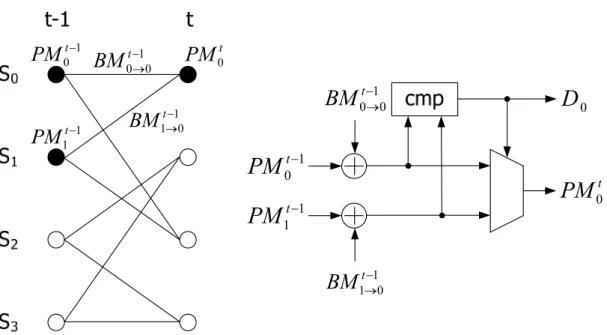
Figure 3.4 shows the 4-state radix-2 trellis and the fundamental radix-2 ACS unit for state S0. As the trellis diagram illustrated, the state S0 has two predecessor states

including S0 and S1. First, the corresponding path metric and branch metric are added.

Then, the two summations are compared to decide which branch is the survivor and which path metric is updated. The new path metric will become the predecessor path

metric at next time instant. Because of the feed-back characteristic, the main speed issue of Viterbi decoder depends on the ACS unit.

1 0 0 t

BM

BM

PM

PM

PM

D

PM

PM

PM

BM

BM

Figure 3.4 The 4-state radix-2 trellis and the radix-2 ACS unit for state S0

3.2.2 High-radix ACS and Two-dimension ACS

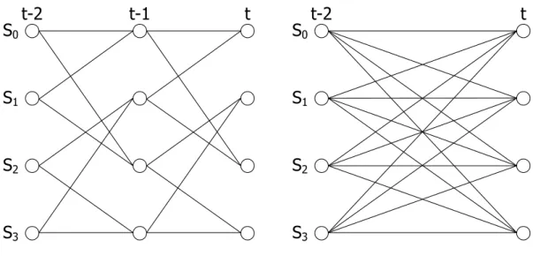
ACS unit is the speed bottleneck of Viterbi decoder due to the feed-back characteristic described in previous subsection. For high speed applications, decreasing the critical path of ACS unit is the most intuitive idea. High-radix ACS structures like radix-4 ACS, radix-8 ACS, radix-16 ACS …, etc. are such strategy. The high-radix structures unroll the ACS loop in order to perform multi-step of the trellis within a single clock period. These lookahead methods replace the fundamental radix-2 trellis with a radix-4 trellis or radix-8 trellis …, etc. For example, a 4-state radix-2 trellis and a 4-state radix-4 trellis are shown in Figure 3.5. Note that the radix-4 ACS trellis in Figure 3.5(b) is formed by combining a two-stage of radix-2 trellis in Figure 3.5(a). For the same clock period, it is clear that the data rate of the radix-4 ACS is two time faster than that of the radix-2 unit. In a similar manner, one can obtain a higher radix trellis diagram.

t-1 S0 S1 S2 S3 t t-2 t S0 S1 S2 S3 t-2

(a) 4-state radix-2 trellis diagram (b) 4-state radix-4 trellis diagram Figure 3.5 The 4-state radix-2 and radix-4 trellis diagrams

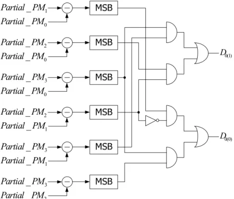
Higher radix trellis must be realized by much larger costs of area. Figure 3.6 shows a radix-4 ACS unit for state S0. This unit computes four sums in parallel

followed by a four-way comparison. The comparison illustrated in Figure 3.7 is realized using six parallel subtractions for minimizing the critical path. Select signal (D0(1) and D0(0)) for 4-to-1 multiplexer can be realized by simple logic gates.

Afterward, the minimum partial path metric is selected as the new path metric. Although the critical path increases, the radix-4 architecture achieves two operation steps per clock period. Consequently, the effective throughput is improved.

2 0 0,0 0 t BM −_{→ →} 2 1 0,0 0 t BM − → → 2 0 t PM − 2 1 t PM − 0 t

PM

D

0 _ Partial PM 1 _ Partial PM 2 _ Partial PM 0 _ Partial PM 3 _ Partial PM 0 _ Partial PM 2 _ Partial PM 1 _ Partial PM 3 _ Partial PM 1 _ Partial PM 3 _ Partial PM 2 _ Partial PM 0(1) D 0(0) D

Figure 3.7 The 4-way comparator in Figure 3.6

For the same clock period, the radix-2τ

ACS unit achieves τ times speed up as compared to the radix-2 ACS unit. Nevertheless, the number of trellis branches will be 2τ-1

times of that in radix-2 trellis, leading to the exponentially increasing complexity. The comparison of different radix-2τ

ACS structures is shown in Table 3.1. The high-radix approach that accelerates Viterbi algorithm can also cause large critical path due to exponentially increasing branches. Among different radix-2τ

ACS structures, radix-4 ACS is a popular choice because of the better compromise between cost and throughput.

Table 3.1 Comparison of different radix-2τ

ACS structures

Radix Throughput Complexity

2 1 1

4 2 2

8 3 4

Although high-radix ACS unit performs multi-step of the trellis within a single clock period, the exponentially increasing complexity causes the difficulty in VLSI implementation. The number of branch metrics generated by the BM unit also increases exponentially. Therefore, a radix-2p_×2q _{structure is introduced to achieve the} throughput equivalent to radix-2τ

approach where τ = p + q. The radix-2p×2q ACS unit, referred to the two-dimension structure, is similar to the radix-2τ

ACS unit, except that only smaller radix-2p ACS unit and radix-2q ACS unit are required. Since the exponentially increasing hardware cost of a high-radix ACS, the complexity of a Viterbi decoder based on radix-2p×2q architecture is much smaller than that based on radix-2τ

architecture. However, the critical path of the two-dimension ACS unit is longer than of radix-2τ

ACS unit. Figure 3.8 shows a 4-state radix-2 trellis and a 4-state radix-2x2 trellis. The structure of radix-2x2 ACS unit for state S0 is shown in

Figure 3.9.

(a) 4-state radix-2 trellis diagram (b) 4-state radix-2×2 trellis diagram Figure 3.8 The 4-state radix-2 and radix-2×2 trellis diagrams

2 0 0 t

BM

BM

PM

PM

PM

BM

BM

PM

PM

BM

BM

Figure 3.9 A radix-2×2 ACS unit

3.3 Path Metric Unit

The path metric unit is the storage element of the accumulative path metric. In VLSI implementation, the path metrics are represented by the memory device with finite length fixed-point device. Path metric normalization is required to prevent the errors due to the overflow during the increasing path metric. The modular normalization technique [3] will be introduced in this section.

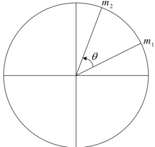
In the modular arithmetic, there is a theorem [4] which can determine the magnitude between two values under some constraints.

Theorem

1 2

2

C m −m <

The theorem as shown in Figure 3.10 describes that the large value is always leading under the constraint that the difference between the two values is less than half of the circumference C.

θ

m

m

Figure 3.10 Circular representation of the modular theorem

According to the Viterbi algorithm, it supposes that the maximum likelihood path would be merged among the truncation length L. Figure 3.11 illustrates this property. In this graph, the t m L and

a PM + + t m L b PM + + _{can be written as} t m L t m a x PM + + =PM + +γa (3.3) t m L t m b x PM + + =PM + +γb (3.4)

Let B denote the maximum difference between two branch metrics which equals to the maximum value of the branch metric. Then the difference of two path metrics in equation (3.3) and equation (3.4) is

t m L t m L

a b a b

PM + + −PM + + = γ −γ ≤BL (3.5)

This equation shows that the difference of any two path metrics is upper bounded by a sum of branch metrics at most L terms. Therefore, the equation is equivalent to the constraint of the modular theorem. According to the modulo theorem, the

b t m L t m L a PM + + ≥PM + + is always satisfied if t m L t m L 0 a b PM + + −PM + + ≥ . t m L a

P M

P M

P M

Figure 3.11 The upper bound of path metric difference

According to the descriptions above, the key idea of the modular normalization is not to avoid the overflow, but to accommodate the overflow. Consequently, the modular normalization is implemented by the 2’s complement adders and subtractors. The representation of path metrics requires b bits to satisfy the constraint

2 2 b t m L t m L a b PM + + ₋PM + + _≤BL_{= (3.6)}

3.4 Survivor Memory Unit

There are two well-know survivor memory management approaches. One is the register-exchange (RE) method and the other is the trace-back (TB) method. The two approaches would be introduced in this section.

3.4.1 Register-exchange Approach

The register-exchange approach is conceptually the simplest used technique which assigns a set of registers to each state. The registers record the corresponding decoded output sequences named survivor paths. For each new time step, the registers may change their contents to update new decoded information. Hence, this approach eliminates the need to trace back since the registers have contained the decoded information. Intuitively, the approach may reduce latency enormously. However, it is not power efficient as a result of the need to shuffle all the registers in a time step to the next time step.

A conventional approach of register-exchange is best state approach [5]. This approach finds out the best path among all paths at each time step. Considering the example introduced in Section 2.2.2, Figure 3.12 shows the decoding process of the best state approach with truncation length 4 over an ideal channel. For each state transition, the content of registers is exchanged according to the survivors labeled by solid lines. And the corresponding information bit labeled with underline is shifted into the leftmost bit of the register. The latency of this example is 4 which equals to the truncation length. Then the decoded bit is stored in the rightmost bit of the register corresponding to the best state. In Figure 3.12, the decoded bit is represented in boldface. For example, the best state at time t=4 is S3. Thus, the decoded bit is ‘1’,

which is the rightmost bit of the register corresponding to S3. The decoded bit for

each time instant can be obtained in a similar way. The realization of this approach is shown in Figure 3.13.

Figure 3.12 The best state approach with truncation length 4

Figure 3.13 Realization of the best state approach

When the truncation length is long enough, all survivor paths of states will merge together at certain time step. In other words, several rightmost bits of all registers contain the same decoded information. In this situation, there is no need to find out the best state. Correspondingly, one can choose the rightmost bit of a fixed state as decoded bit. The decoding process of fixed state approach with truncation length 4 is shown in Figure 3.14. Choosing state S0 to obtain the decoded output, the register

the rightmost bit of the register. Note that at any time step in this example, the rightmost bits of each state are the same. The realization of this approach is shown in Figure 3.15. This approach doesn’t need to find out the best state. However, more registers are required to save longer survivor path.

Figure 3.14 The fixed state approach with truncation length 4

A compromising approach between best state approach and fixed state approach is labeled as majority vote approach [6]. Compared with the best state approach, this approach replaces the find-best-state unit with majority vote circuit. If the number of 1’s of the rightmost bits is larger than the number of 0’s, the decoded bit is 1. Otherwise, the decoded bit is 0. The decoding process of majority vote approach with truncation length 4 and its realization are shown in Figure 3.16 and Figure 3.17, respectively.

Figure 3.16 The majority vote approach with truncation length 4

3.4.2 Trace-back Approach

The trace-back approach has been introduced in Section 2.2.2. Unlike register-exchange approaches, one does not need to store the information sequence but only stores the results of each comparison in memory. After a certain number of branches which depends on the truncation length have been processed, these trellis connections are recalled in reverse order. The path which is traced back through the trellis diagram is used to determine the decoded information bits. This decoding process is called the trace-back approach. Although trace-back approach will increase overall hardware latency, it consumes less power and suits for portable applications. There are three types of operations performed inside a trace-back approach.

z Write (WR):

The decisions made by the ACS unit are written into memory locations corresponding to each state. The write pointer moves forward as ACS operations move from one time step to the next in trellis.

z Trace-back (TB):

When the decoding process goes forward with trellis diagram, one must trace back the trellis on the best path metric. The pointer values from this operation are not the decoded sequence but the maximum likelihood path. Certain iterations are needed to ensure that the trace back path reaches merging state with high probability so that actual decoding process may come up. According to the Viterbi algorithm, the trace-back operation is usually run to a predetermined truncation length L before the decoding operation.

z Decode (DC):

When the trace-back operation finishes, a merging state is determined. Then, a decoding operation begins to generate the decoded bits in a reverse order. This operation proceeds in exactly the same fashion as the trace-back operation. Pointer

values from this operation are the decoded values and are temporarily stored in a last-in first-out (LIFO) memory, and sent out when decoding operation finishes.

The trace-back approach is called k-pointer approach if there are k read pointers operating simultaneously. In the k-point approach, read and write operations proceed in parallel using several memory banks. That is, write, trace-back, and decode operations are performed in different memory banks at the same time.

Figure 3.18 shows the memory structure and operation of k-pointer odd approach with k=3. There are 2k-1 memory banks, each of size

1

L N

k− × , where N is the

number of states and L is the truncation length of trellis. Since the truncation length L must be achieved before decoding, two read pointer perform the trace-back operation in two memory banks and one more read pointer performs the decode operation in one memory bank. First of all, write operation is executed. After write operation is completed in the third memory bank, the read pointer starts trace-back operation in the third memory bank at the best path metric. At the same time, write operation continues in the fourth memory bank. The trace-back operation continues across the third and the second banks, while the ACS decisions are written to the fourth and the fifth banks. Note that the combined length of the second and the third banks is exactly the truncation length L. Hence, a merging state at the first memory bank is determined by trace-back operation of length L. Then, the decoding operation starts and the decoded bits are generated in reverse order. Furthermore, the new decisions from ACS unit can be written to the first memory bank at once. The latency of the k-pointer approach is 2

1

k L

k− , which is the time delay from writing the first column to

decoding the first symbol. In this example of 3-pointer odd algorithm, the latency is 3L as shown in Figure 3.18. With this decoding process, one can generate the decoded bits sequentially.

Figure 3.18 Memory structure and operation of the 3-pointer odd approach

Figure 3.19 shows the memory structure and operation of k-pointer even approach with k=3. There are 2k memory banks, each of size

1

L N

k− × . The decoding process

of the k-pointer even approach is similar to the k-pointer odd approach. The main difference is that the k-pointer even approach needs one more memory banks because decoding operation and write operation are divided into two memory banks.

Figure 3.19 Memory structure and operation of the 3-pointer even approach

The one-pointer approach differs significantly from the k-pointer approach. This approach adopts only one read pointer but needs to speed up the read operation. For example, if a k-pointer approach is converted to one-pointer approach, the trace-back and decoding operations need to be performed k times faster. However, the number of memory banks can be reduced. Figure 3.20 shows the memory structure and operation of one-pointer approach with k=3. First, write operation is executed. After write operation is completed in the third memory bank, the read pointer starts trace-back operation in the third memory bank at the best path metric. At the same time, write operation continues in the fourth memory bank. Notice that the read operation is 3 times faster than the write operation. Therefore, when the write operation finishes in

the fourth memory bank, the trace-back and decoding operation must be completed in the other three memory banks. By a similar fashion, the decoded bits can be generated sequentially. Furthermore, the number of memory banks and latency of this example are 4 and 2L respectively, which are smaller than those of the 3-pointer approach. In conclusion, if a k-pointer approach is converted to one-pointer approach, k+1 memory banks are needed, each of size

1

L N

k− × , and the latency is 1 1 k L k + − . 1 L/2 1 L/2 1 L/2 1 L/2 L/2 L Time 3L/2 2L 5L/2 3L 4L 7L/2

: Write : Trace-back : Decode

Figure 3.20 Memory structure and operation of the one-pointer even approach

The hybrid trace-back approach combines the k-pointer approach and one-pointer approach. That is, the trace-back and decoding operations become k1 times faster to determine the merging state and decoded bits, which is like the one-pointer approach.

1

In addition, it uses k2 read pointers simultaneously when trace-back and decoding operations are executed, which is like the k-pointer approach. Figure 3.21 shows the memory structure and operation of even hybrid approach with k1=2 and k2=2. In this approach, the number of memory banks are k k₂( ₁+ − and 1) for the odd hybrid approach and the even hybrid approach, respectively. Each memory bank size is 2( 1 1 k k + ) 1 2 1 L N

k k − × . And the latency is

2 1 1 2 ( 1) 1 k k L k k + − .

Chapter 4

Some low-power Schemes for Viterbi

Decoder

In this chapter, we will introduce some low power schemes for Viterbi decoder. The first one is scarce-state-transition (SST) algorithm proposed in 1987. As the channel noise is not serious, SST technique reduces the switching activity of the input sequence significantly. Next, we will describe adaptive Viterbi algorithm, which is a popular low-power scheme for Viterbi decoder. Unlike conventional Viterbi algorithm, adaptive Viterbi algorithm applies the path-pruning technique to reduce computation and storage requirements. Finally, we will propose a modified memory management based on path merging property of Viterbi algorithm. This scheme provides variable truncation length for register-exchange approach to access the survivor memory efficiently.

4.1 Scarce-State-Transition (SST) Algorithm

The scarce-state-transition (SST) algorithm [7] [8] [9] was first proposed by Ishitani et al in 1987. It is a low-power technique for Viterbi decoder to reduce the state transition activity significantly under high SNR condition. The decoding process of SST algorithm will be introduced in this section.

Figure 4.1 shows the block diagram and data sequences of convolutional code. In this block diagram, denotes the information sequence,

is the codeword sequence deriving from the generator polynomial . From the

( )

u D C D( )=u D G D( )⋅ ( )

( )

received sequence , the Viterbi decoder estimates the decoded information sequence . ( ) r D ( ) o D

Figure 4.1 The block diagram of convolutional code

The SST Viterbi decoding model illustrated in Figure 4.2 includes two additional blocks: pre-decoder and re-encoder. The re-encoder is the same as the convolutional encoder of the transmitter and the pre-decoder provides the inverse function of the convolutional encoder. The SST decoding scheme consists of some steps. First, the hard decision of the received sequence is pre-decoded by the pre-decoder. Next, the output of the pre-decoder is re-encoded by the convolutional encoder. The modulo-2 addition of the received sequence and the re-encoded sequence is the new input of the Viterbi decoder. Finally, the decoded information sequence is the modulo-2 addition of the output of Viterbi decoder and the output of the pre-decoder.

Figure 4.2 The model of SST Viterbi decoding

The relationships between the data sequence in Figure 4.2 are described as follows. The received sequence can be expressed as

(4.1)

( ) ( ) ( ) ( ) ( ) ( )

r D =u D G D⋅ +e D =C D +e D

where is the error sequence from a noisy channel. Next, the pre-decoder directly decode the information sequence from by perform the inverse

( )

e D

( )

function of the encoder. The output of pre-decoder is

(4.2)

1 _ˆ

( ) ( ) ( ) ( )

i D ₌r D G_⋅ − D ₌u D

The re-encoder then encodes i D( ) to a new codeword sequence z(D)

(4.3)

ˆ ( ) ( ) ( ) ( )

z D =i D G D⋅ =C D

The new input sequence of the Viterbi decoder equals to the modulo-2 addition of the received sequence and the re-encoded sequence, which is represented as ( ) y D (4.4) ˆ ( ) ( ) ( ) ( ) ( ) ( ) y D =r D +z D =C D +e D +C D

The Viterbi decoder then performs maximum likelihood decoding on . From equation (4.4), it is obvious that the switching activity of depends on the channel noise. In high SNR condition, the input of the Viterbi decoder is nearly zero as well as the output of the Viterbi decoder . The decoded information sequence equals to the modulo-2 addition of the output of Viterbi decoder and the output of the pre-decoder, which can be represented as

( ) y D ( ) y D ( ) y D ( ) n D ( ) o D (4.5) ˆ ( ) ( ) ( ) ( ) ( ) o D =i D +n D =u D +n D

Figure 4.3 illustrates the SST decoding process for the (2, 1, 2) convolutional code described in Section 2.1.1. Assume the encoder has reset to the 00 state, the encoded codeword symbols corresponding to information bit 0 and information bit 1 are (0,0) and (1,1) respectively. In BPSK modulation, the coded bit ‘0’ is mapped to ‘+1’ and ‘1’ is mapped to ‘-1’. As the codeword symbols pass through the noisy channel, the received symbols may not match the codeword symbols due to the errors denoted by e in Figure 4.3. In this example, 3-bit quantization is applied to represent the received symbol. Then, the hard decision of the received symbol is processed by the pre-decoder and re-encoder. As Figure 4.3 illustrated, the input of the Viterbi decoder becomes the error symbol e introduced by channel noise. The output of the Viterbi decoder is expected to be zero as the channel noise is not serious. Finally, the

decoded information bit which is the same as that in the transmitter is obtained.

Figure 4.3 The SST Viterbi decoding process

The SST algorithm has the following properties. As the channel noise is not serious, most of the decoded bits of the Viterbi decoder are zero. Therefore, the survivor path will pass through the zero state at most of the time and the zero state is most likely the best state with minimum path metric. Figure 4.4 shows the survivor paths of the conventional Viterbi algorithm and the SST algorithm over a noiseless channel. For conventional Viterbi algorithm, the maximum likelihood state is distributed across all the states. On the other hand, the zero state has a higher probability to be the maximum likelihood state than other states as SST algorithm is exploited. This property is useful for the modified memory management we proposed, which will be described later.

(a)Conventional Viterbi algorithm

(b)SST algorithm

Figure 4.4 The survivor paths over a noiseless channel

The SST algorithm performs a transformation process that converts the origin input sequence of the Viterbi decoder into an approximately zero sequence as the channel condition is good enough. As a result, the state transition activity is reduced and the decoded sequence passes through the zero state with high probability under high SNR environment. Therefore, the dynamic power is reduced as the channel becomes better.

4.2 Adaptive Viterbi Algorithm

Adaptive Viterbi algorithm [10] [11] combines the Viterbi algorithm with the principle of T-algorithm [12]. Unlike conventional Viterbi algorithm which retains all survivors of each state at each trellis stage, T-algorithm applies the path-pruning technique to reduce computation and storage requirements. Instead of computing and retaining all possible paths, only some paths which satisfy certain path-cost conditions are retained at each stage. The path retention is based on the following criteria

z A path is retained if its path metric is less than d_m + , where T is a threshold T

value determined by the designer and is the best path metric among all survivor paths at the previous trellis stage.

m d

z The total number of survivor paths per trellis stage is limited to a fixed number , which is also determined by the designer and less than the state number.

max N

The first criterion allows high-cost paths to be eliminated in the decoding process. In the case of many paths with similar cost, the second criterion restricts the number of paths to . At each stage, the minimum path metric , threshold T, and maximum survivor number are used to prune the number of survivor paths.

max

N d_m

max N

For adaptive Viterbi algorithm, it is important to select T and carefully. If threshold T is set to a small value, the average number of paths retained at each trellis stage will be reduced. However, the bit error rate may increase since the most likely path has to be taken from a reduced number of possible paths. Alternatively, if a large value of T is selected, the average number of retained paths increases and results in a reduced bit error rate. But the computation and the path-storage requirements also increase. The maximum number of survivor paths per stage , has a similar effect on bit error rate as T. Therefore, an optimal value for T and should be chosen

max N max N max N

so that bit error rate is within allowable limits, while matching the resource of the hardware. Figure 4.5 shows the ACS unit of adaptive Viterbi decoder.

Adder

d

<d

+T

Number

of paths

= count

Y

N

Discard path

count

< N

N

Discard path

Y

To survivor

memory

Figure 4.5 The ACS unit of adaptive Viterbi decoder

4.3 Variable Truncation Length

As Section 3.4 mentioned, there are two well-know survivor memory management approaches: the register-exchange (RE) approach and the trace-back (TB) approach. Register-exchange approach is conceptually the simplest used technique and eliminates the need to traceback since the registers have contained the decoded information. Compared with trace-back approach, register-exchange approach has the advantage of short critical path, short latency, and simple structure. However, register-exchange method is not power efficient due to the need to copy the contents of all registers in a stage to the next stage. In this Section, we will propose a modified memory management based on path merging property of Viterbi algorithm. This scheme provides variable truncation length for register-exchange approach to access the survivor memory efficiently. Figure 4.6 illustrates a 64-state Viterbi decoder with radix-2x2 ACS and RE-based survivor memory.

Ro ut in g Ro ut in g Ro ut in g

Figure 4.6 A 64-state, radix-2x2 Viterbi decoder with RE-based memory

In Section 2.23, we introduce an important characteristic of Viterbi algorithm, namely path merging property. As path merging property mentioned, all survivor paths will merge with high probability if the truncation length L is long enough. By selecting proper truncation length, the decoded data can be determined with L-stage information only. Moreover, it is unnecessary to search for the best state. In fact, the decoded data from any state is the same if all survivor paths have merged. Based on this characteristic, fixed state approach is a proper choice for a register-exchange based survivor memory when the state number is large.

As all survivor paths merge, it is more efficient to store the merged path rather than all paths. Based on this principle, we propose a low-power scheme called variable truncation length for Viterbi decoder. Figure 4.7 illustrates a 64-state, radix-2x2, RE-based survivor memory with variable truncation length. D0 to D63 are

the decisions provided by the ACS units for selecting survivor paths. In the decoding process, the contents of registers corresponding to 64 states tend to be equivalent from the left stages to the right stages. The registers of each stage are connected to the

path merging detection unit. The path merging detection unit will find the merged stage in the memory and generates clock gating signals of each stage to eliminate unnecessary data movement.

D1 D62 D63 OUT D2 CLK0 CLK1 CLK2 D0 2'b00 Clock Gating CLK3

Path Merging Detection Unit

Figure 4.7 A RE-based survivor memory with variable truncation length

Figure 4.8 illustrates the survivor memory by trellis diagram. In this example, the fixed state approach is applied and the decoded data is obtained from state 0. After detecting the merged point, we apply clock gating to the registers in the shadow region and directly shift out the value of state 0. The path corresponding to state 0 is considered as the correct one, and the others are dropped. Based on the scheme, we can adjust truncation length dynamically, depending on the channel. In high SNR environments, a shorter truncation length is required and the clock gating can be