Particle Interactions in Diffusiophoresis and Electrophoresis of Colloidal Spheres with Thin but Polarized Double Layers

Particle Interactions in Diffusiophoresis and Electrophoresis of Colloidal

Spheres with Thin but Polarized Double Layers

Hung J. Tu and Huan J. Keh1

Department of Chemical Engineering, National Taiwan University, Taipei 106-17, Taiwan, R.O.C.

Received March 10, 2000; accepted August 4, 2000

The diffusiophoretic and electrophoretic motions of two colloidal spheres in the solution of a symmetrically charged electrolyte are analyzed using a method of reflections. The particles are oriented arbitrarily with respect to the electrolyte gradient or the electric field, and they are allowed to differ in radius and in zeta potential. The thickness of the electric double layers surrounding the particles is assumed to be small relative to the radius of each particle and to the gap width between the particles, but the effect of polarization of the mobile ions in the diffuse layer is taken into account. A slip velocity of fluid and normal fluxes of solute ions at the outer edge of the thin double layer are used as the boundary conditions for the fluid phase outside the double layers. The method of reflections is based on an analysis of the electrochemical potential and fluid velocity disturbances produced by a single dielectric sphere placed in an arbitrarily varying electrolyte gradient or electric field. The solution for two-sphere interactions is obtained in expansion form correct to O(r−7₁₂), where r12is the distance between the particle

centers. Our analytical results are found to be in good agreement with the available numerical solutions obtained using a boundary collocation method. On the basis of a model of statistical mechan-ics, the results of two-sphere interactions are used to analytically determine the first-order effect of the volume fraction of particles of each type on the mean diffusiophoretic and eletrophoretic veloci-ties in a bounded suspension. For a suspension of identical spheres, the mean diffusiophoretic velocity can be decreased or increased as the volume fraction of the particles is increased, while the mean electrophoretic velocity is reduced with the increase in the particle concentration. Generally speaking, the particle interaction effects can be quite significant in typical situations. °C2000 Academic Press

Key Words: diffusiophoresis; electrophoresis; two-sphere

interac-tion; particle concentration effect; thin but polarized double layer.

1. INTRODUCTION

The transport behavior of small particles in a continuous medium at low Reynolds numbers is of much fundamental and practical interest. In general, driving forces for motions of col-loidal particles include concentration gradients of the particles themselves (diffusion), bulk velocities of the disperse medium

1_{To whom correspondence should be addressed. Fax: +886-2-2362-3040.}

E-mail: huan@ccms.ntu.edu.tw.

(convection), and gravitational or centrifugal fields (sedimen-tation). Problems of the colloidal transport induced by these well-known driving forces were treated extensively in the past. Another category of driving forces for the locomotions of col-loidal particles involves a nonuniform imposed field (such as electric potential, temperature, or solute concentration) that in-teracts with the surface of each particle. The particle motions associated with this mechanism, known as “phoretic motions,” have received a considerable amount of attention recently (1–3). Perhaps the most familiar example of various phoretic mo-tions is electrophoresis, which results from the interaction be-tween an external electric field and the electric double layer surrounding a charged particle, and is widely used for the parti-cle characterization and separation in a variety of colloidal and biological systems. The electrophoretic velocity U(0)_{of a single} nonconducting particle suspended in an unbounded electrolyte solution is simply related to the uniformly applied electric field

E∞by the Smoluchowski equation (4, 5),

U(0)= εζ

4πηE

∞_{. [1.1]}

Here,ε/4π is the fluid permittivity, η is the fluid viscosity, and

ζ is the zeta potential of the particle surface.

Another example of phoretic motions is diffusiophoresis, which is the migration of a particle in response to the macro-scopic concentration gradient of a solute, and was applied to certain latex-particle coating processes (6). The particle moves toward or away from a region of higher solute concentration, depending on some long-range interactions between the solute molecules and the particle. In an unbounded solution of a sym-metrically charged binary electrolyte with a constant concentra-tion gradient∇n∞, the diffusiophoretic velocity of a charged particle is (7) U(0)= εζ 4πη kT Z e ∇n∞ n∞(0) · D2− D1 D2+ D1 +4kT Z eζ ln cosh µ Z eζ 4kT ¶¸ . [1.2]

Here, n∞(0) is the macroscopic electrolyte concentration mea-sured at the particle center 0 in the absence of the particle, D1 and D2 are the diffusion coefficients of the anion and cation,

265 0021-9797/00 $35.00

Copyright°C2000 by Academic Press All rights of reproduction in any form reserved.

respectively, Z is the absolute value of the valences of ions, e is the charge of a proton, k is the Boltzmann constant, and T is the absolute temperature. For the special case of D2 = D1, Eq. [1.2] predicts that the particle movement (due to chemiphoresis only) is in the direction of increasing electrolyte concentration re-gardless of the sign ofζ and the particle velocity is a monotonic increasing function of the magnitude ofζ .

Equations [1.1] and [1.2] indicate that the electrophoretic and diffusiophoretic velocities of a dielectric particle having a uni-form zeta potential on its surface are independent of the particle size and shape (and there is no rotational motion of the parti-cle). However, their validity is based on the assumptions that the local radii of curvature of the particle are much larger than the thickness of the electric double layer at the particle surface and that the effect of polarization (relaxation effect) of the diffuse ions in the double layer due to nonuniform “osmotic” flow is negligible. In fact, important advances were made in the past in the evaluation of the phoretic velocities of colloidal particles relaxing these assumptions.

Taking the double-layer distortion from equilibrium as a per-turbation, O’Brien and White (8) obtained a numerical calcula-tion for the electrophoretic velocity of a dielectric sphere of ra-dius a in a KCl solution which was applicable to arbitrary values ofζ and κa, where κ−1is the Debye screening length [equal to (εkT/8π Z2e2n∞)12]. On the other hand, Dukhin and Derjaguin (6) obtained an analytical expression for the electrophoretic mo-bility of a spherical particle surrounded by a thin but polarized double layer in the solution of a symmetrically charged elec-trolyte. Later, O’Brien (9) generalized this analysis to the case of electrophoretic motion of a colloidal sphere in the solution containing an arbitrary combination of electrolytes. The essence of this thin-layer polarization approach is that a thin diffuse layer can still transport a significant amount of solute molecules so as to affect the solute transport outside the diffuse layer. The result for the electrophoretic velocity of a sphere with a thin but polarized double layer in a symmetric electrolyte solution can be expressed as (10) U(0)= εζ 4πηE ∞·1 3(2+ c1+ c2) + 4kT 3Z eζ(c1− c2) ln cosh µ Z eζ 4kT ¶ ¸ , [1.3] where coefficients c1 and c2 are functions of κa defined by Eqs. [2.15a] and [2.15b]. A comparison of Eq. [1.3] with the numerical results for the KCl solution shows that the thin-layer polarization model is quite good over a wide range of zeta po-tentials whenκa > 20. If Ze|ζ|/kT is small and κa is large, the interaction between the diffuse counterions and the particle surface is weak and the polarization of the double layer is also weak. In the limit of

(κa)−1exp µ Z e|ζ | 2kT ¶ → 0, [1.4]

c1= c2=1₂ and Eq. [1.3] reduces to the Smoluchowski equation [1.1]. In general, the electrophoretic velocity given by Eq. [1.3] is not a monotonic function ofζ for a finite value of

κa, unlike the prediction of Eq. [1.1].

In contrast, Prieve and Roman (11) obtained a numerical so-lution of the diffusiophoretic velocity over a broad range ofζ andκa for a charged sphere in concentration gradients of sym-metric electrolytes (KCl or NaCl) using the method of O’Brien and White (8). Recently, analytical expressions for the velocity of a dielectric sphere with a thin but polarized double layer un-dergoing diffusiophoresis in electrolyte solutions have also been derived (3, 12). The result for this diffusiophoretic velocity in a symmetric electrolyte solution is

U(0)= εζ 4πη kT Z e ∇n∞ n∞(0) · 2 3 µ D2− D1 D2+ D1 + b1− b2 ¶ + 8kT 3Z eζ(1+ b1+ b2) ln cosh µ Z eζ 4kT ¶¸ , [1.5] where b1and b2are coefficients related to (D2− D1)/(D2+ D1) andκa defined by Eq. [2.31]. When κa > 20, the agreement be-tween Eq. [1.5] and the numerical solution is excellent for all reasonable values of the zeta potential. In the limiting situation as given by Eq. [1.4], the effect of double-layer polarization dis-appears and Eq. [1.5] reduces to Eq. [1.2]. Even for the case of D2= D1, the particle velocity given by Eq. [1.5] for a finite value of κa may not be a monotonic function of the magni-tude ofζ and its direction can reverse (toward lower electrolyte concentration) when|ζ| becomes large.

It could be found from Eqs. [1.3] and [1.5] that the effect of polarization of the diffuse layer is to decrease the particle velocity. The reason for this consequence is that the transport of the diffuse ions within the double layer reduces the local electrolyte gradient or electric field along the particle surface. Numerical calculations of Eqs. [1.3] and [1.5] show that even whenκa is as large as 300 the effect of ion transport inside the diffuse layer cannot be ignored if|ζ | equals several kT/e.

In practical applications of diffusiophoresis and electrophore-sis, collections of particles are usually encountered, and effects of particle interactions will be important. In the limiting case that Eqs. [1.1] and [1.2] are applicable, the normalized velocity field of the immense fluid that is dragged by a particle during diffusiophoresis is the same as for electrophoresis of the parti-cle (1); thus, the partiparti-cle interaction effects in electrophoresis under the situation of infinitesimally thin double layer (satisfy-ing Eq. [1.4]), which were studied extensively in the past (2, 13–16), can be taken to interpret those in diffusiophoresis. An important result of these studies is that the diffusiophoretic or electrophoretic velocity of each particle is unaffected by the presence of the others if all of the particles in the unbounded solution have the same zeta potential.

When the polarization effect of diffuse ions in the dou-ble layers surrounding the particles is considered, the particle

interaction behavior in diffusiophoresis can be quite different from that in electrophoresis, due to the fact that the particle size and some other factors are involved in each transport mecha-nism (3). Through the use of a boundary collocation method, the electrophoresis of multiple spheres with thin but polarized double layers in an arbitrary configuration was examined (10, 17). Recently, the thin-layer polarization model and the bound-ary collocation technique were also used to investigate the ax-isymmetric diffusiophoresis of a chain of dielectric spheres in electrolyte solutions (18). In these studies, numerical results of the electrophoretic and diffusiophoretic velocities of the parti-cles were presented for various cases. It was found that partiparti-cles with the same zeta potential do interact with one another, un-like the no-interaction results obtained in previous investigations neglecting the polarization effect of the double layers.

Until now, the interactions between particles undergoing dif-fusiophoresis in asymmetric configurations allowing the polar-ization of the diffuse ions in the double layers have not been examined. The main object of the present work is to analyti-cally study the diffusiophoretic and electrophoretic motions of two charged colloidal spheres surrounded by polarized diffuse layers in a constant electrolyte gradient or electric field oriented arbitrarily with respect to the line through particle centers. The particles, which are freely suspended in the fluid solution, may have arbitrary radii and zeta potentials. It is assumed that the thickness of the double layers is small relative to the radius of each particle and to the surface-to-surface distance between the particles. A method of reflections is used to solve the quasi-steady problem.

In the next section we consider the local electrochemical po-tential and fluid velocity fields produced by a single spherical particle placed in a prescribed electrolyte concentration field whose gradient is not necessarily constant over length scales comparable to the particle radius. It is shown that Eq. [1.5] (or Eq. [1.3]) also applies to a single sphere in a nonuniform elec-trolyte gradient (or electric field), provided that∇n∞(or E∞) is evaluated at the position of the particle center. These results are then used in Section 3 to alternately evaluate the effects of one sphere on the other in a constant applied electrolyte gradient. The translationl and angular velocities of the diffusiophoretic particles are determined in this reflection manner with an error of O(r₁₂−8), where r12is the center-to-center distance between the particles, and the results are given in Eq. [3.9]. In Section 4 our analytical results are compared with the numerical calculations obtained using the boundary collocation method for the case of two diffusiophoretic spheres oriented parallel to the undisturbed electrolyte gradient. Typical effects of the particle and electrolyte properties on the two-sphere interactions in asymmetric diffu-siophoresis are discussed. In Section 5, the results of two-sphere interactions derived in Section 3 for an arbitrary configuration are applied to a theory of particle concentration effects on trans-port properties in dilute dispersions to obtain the effect of the volume fraction of particles of each type on the average diffu-siophoretic velocities in a bounded suspension, and the general

result is given in Eqs. [5.8] and [5.9]. Finally, in Section 6, the analytical solutions for the electrophoretic motions of a single dielectric sphere in an arbitrary electric field, of two spheres in a constant electric field, and of a suspension of spheres, which can be obtained by the same approach used for the diffusiophoresis in the previous sections with only minor changes, are presented. For the electrophoresis of two spheres with the line through their centers parallel and perpendicular to the applied electric field, the numerical calculations obtained using the collocation method are employed to compare our reflection results.

2. A SINGLE CHARGED SPHERE IN AN ARBITRARY CONCENTRATION FIELD OF A

SYMMETRIC ELECTROLYTE

For the purpose of obtaining the interactions between two spherical dielectric particles undergoing diffusiophoresis in a solution of a symmetrically charged binary electrolyte by the method of reflections, it is necessary to understand the motion of a single sphere in an unbounded solution with an arbitrary concentration field nA(x). The instantaneous center of the par-ticle with uniform zeta potentialζ is positioned at x0, and the relative position vector is defined as r= x − x0 (=rer, where er is the unit vector in the direction of r). Although x0changes with time, the problem can be dealt with as a quasi-steady state if both the Peclet number and the Reynolds number are van-ishingly small. It is assumed that the polarized electric double layer surrounding the particle is thin in comparison with the par-ticle radius a (say,κa > 20) and that a|∇nA|/nA(x0)¿ 1 in the vicinity of the particle.

The fluid phase can be divided into two regions: an “inner” region defined as the thin double layer adjacent to the parti-cle surface and an “outer” region defined as the remainder of the fluid, which is electrically neutral. In the outer region, the equations of conservation of each ionic species and the fluid momentum are the Laplace equation (3),

∇2_µ

m= 0, m= 1, 2, [2.1]

and the Stokes equations,

η∇2_{v− ∇ p = 0, [2.2a]}

∇ · v = 0. [2.2b]

In Eq. [2.1],µm(x) is the electrochemical potential energy of

ionic species m defined as

µm= µ0m+ kT ln nm+ zme8, [2.3]

whereµ0

mis a constant, nm(x) and zmare the concentration and

valence, respectively, of type-m ions, and8(x) is the electric potential. m equal to 1 and 2 refer to the anion and cation, re-spectively, so−z1= z2= Z > 0. In Eq. [2.2], v(x) is the fluid

velocity and p(x) is the dynamic pressure. Note that both nm

and8 also satisfy Laplace’s equation.

The governing equations [2.1] and [2.2] in the outer region satisfy the following boundary conditions at the particle surface (r = a+, the outer edge of the thin double layer) obtained by solving for the electrochemical potentials and fluid velocity in the inner region and using a matching procedure to ensure a continuous solution in the whole fluid phase (3, 9),

r = a+: er· ∇µm= − 2 X i₌₁ βmiI :∇s∇sµi, m = 1, 2, [2.4] v= vS≡ U + Ω × r + v(s), [2.5]

where the relaxation coefficients

β11 = 1 κ · 4 µ 1+3 f1 Z2 ¶ exp( ¯ζ ) sinh ¯ζ −12 f1 Z2 ( ¯ζ + ln cosh ¯ζ) ¸ , [2.6a] β12 = − 1 κ µ 12 f1 Z2 ¶ ln cosh ¯ζ , [2.6b] β21 = − 1 κ µ 12 f2 Z2 ¶ ln cosh ¯ζ , [2.6c] β22 = 1 κ · −4 µ 1+3 f2 Z2 ¶ exp(−¯ζ) sinh ¯ζ −12 f2 Z2 ( ¯ζ − ln cosh ¯ζ) ¸ , [2.6d]

and the apparent slip velocity

v(s)= − ε

2πη

kT

(Z e)2[( ¯ζ + ln cosh ¯ζ)∇sµ1

+ (−¯ζ + ln cosh ¯ζ)∇sµ2]. [2.7]

In Eqs. [2.4]–[2.7], ¯ζ = Zeζ/4kT ; fm= εk2T2/6πηe2Dm; I

is the unit dyadic;∇s= (I − erer)· ∇ denotes the gradient op-erator along the particle surface; U andΩ are the instantaneous translational and angular velocities, respectively, of the particle to be determined. To obtain Eqs. [2.4]–[2.7], it was assumed that the concentration of each ionic species within the double layer is related to the electric potential by a Boltzmann distribution. The polarization effect arising in Eq. [2.4] allows for the diffusion and electric migration of the ions in the bulk solution into the double layer, where they are dispersed in the direction parallel to the particle surface. In the limiting situation as given by Eq. [1.4] (no polarization of the double layer),βmi/a = 0 and the

elec-trochemical potentials in the outer region are independent of the dynamics within the double layer.

The electrochemical potentials far away from the particle ap-proach the undisturbed values and the fluid is motionless there.

Thus,µmand v must obey

r→ ∞: µm→ µm A= µ0m+ kT · 1−zm Z µ D2− D1 D2+ D1 ¶¸ ln nA, m= 1, 2, [2.8] v→ 0. [2.9]

The second term in the brackets of Eq. [2.8] represents the con-tribution from the macroscopic electric field induced by the dif-ference of ion diffusion rates (7, 19). It is obvious that∇2_n

A = 0

and∇2_µ

m A= 0.

A general solution to Eq. [2.1] that satisfies Eq. [2.8] is

µm= µm A+ ∞ X n=1 µ a r ¶n+1 Sn[·]λmn, m= 1, 2. [2.10]

Here, the nth-order polyadic Snis a surface harmonic, defined by

Sn= rn+1∇n(r−1), λmn are nth-order polyadic constants, and

the symbol [·] represents n scalar products using the inner nest-ing convention. Substitution of Eq. [2.10] into Eq. [2.4] leads to

λm1 = − 2 X i=1 gmia(∇µi A)0, [2.11] λm2 = 1 3 2 X i₌₁ hmia2(∇∇µi A)0, [2.12] where g11= 1 2(c 0 1+ c1), g12= 1 2(c 0 1− c1), [2.13a–d] g21= 1 2(c 0 2− c2), g22= 1 2(c 0 2+ c2), h11= 1 2(d 0 1+ d1), h12 = 1 2(d 0 1− d1), [2.14a–d] h21= 1 2(d 0 2− d2), h22 = 1 2(d 0 2+ d2), with c1 = 1 2a21 1

(a2−2aβ11+3aβ12+aβ22+2β12β21−2β11β22), [2.15a]

c2 = 1 2a21

1

(a2−2aβ22+3aβ21+aβ11+2β12β21−2β11β22), [2.15b] c₁0 = c1− 3 β 12 a11 , c₂0 = c2− 3 β 21 a11 , [2.15c,d]

d1= 1 3a2₁

2

(a2− 3aβ11+ 5aβ12+ 2aβ22

+ 6β12β21− 6β11β22), [2.16a]

d2= 1 3a21

2

(a2− 3aβ22+ 5aβ21+ 2aβ11

+ 6β12β21− 6β11β22), [2.16b] d₁0 = d1− 10β12 3a12 , d₂0 = d2− 10β21 3a12 , [2.16c,d] 11 = 1 a2(a 2_{+ aβ} 11+ aβ22− β12β21+ β11β22), [2.17] 12 = 1 a2(a 2_{+ 2aβ} 11+ 2aβ22− 4β12β21+ 4β11β22), [2.18] and the subscript 0 to variables inside parentheses denotes evaluation at x= x0. Substituting Eqs. [2.11] and [2.12] into Eq. [2.10], we obtain µm= µm A+ 2 X i=1 · gmi µ a r ¶3 r· (∇µi A)0 + hmi µ a r ¶5 rr : (∇∇µi A)0+ O(∇∇∇µi A)0 ¸ . [2.19]

In the limit of Eq. [1.4], Eqs. [2.13]–[2.16] reduce to c1=

c2= c10 = c02= g11= g22= 1/2, d1= d2= d10 = d20 = h11=

h22 = 1/3, and g12 = g21 = h12= h21 = 0.

A solution to Eqs. [2.2], [2.5], and [2.9] for the velocity field can be constructed from Lamb’s general solutions as outlined by Brenner (20). The fluid velocity is completely specified when the polyadic coefficientsαn, βn, and γnin the following formulas

are calculated using the value of the velocity field on the surface of the particle (vS): er· vS= ∞ X n=1 αn[·]Sn, [2.20a] −a∇ · vS= ∞ X n=1 βn[·]Sn, [2.20b] aer · (∇ × vS)= ∞ X n₌₁ γn[·]Sn. [2.20c]

The force and torque exerted by the surrounding fluid on the surface r = a+are given by

F= 2πηa(3α1+ β1), [2.21a]

T= 4πηa2γ1. [2.21b]

Since the particle is freely suspended in the fluid, the velocities

U andΩ are obtained by setting the above expressions for F and T equal to zero.

Substitution of Eq. [2.5] into the left-hand side of Eq. [2.20c] leads to

γ1 = −2aΩ, [2.22a]

γn = 0 for n> 1. [2.22b]

By setting T= 0 and using Eqs. [2.21b] and [2.22a], one finds

Ω= 0, [2.23]

as the general result for a prescribed field µm A as long as ∇2_µ

m A= 0.

The translational motion is described by the coefficientsαn

andβn. It can be obtained from Eqs. [2.5] and [2.20a] that

α1 = −U, [2.24a]

αn = 0 for n> 1. [2.24b]

Finally, substituting Eq. [2.5] together with Eqs. [2.7] and [2.19] into Eq. [2.20b] and neglecting the terms of O(∇∇∇µm A)0(only

β1andβ2are needed in the following calculations), one has

β1 = 3 2 X m=1 Gm(∇µm A)0, [2.25a] β2 = 2a 2 X m=1 Hm(∇∇µm A)0, [2.25b] where G1= εkT 3πη(Ze)2[(1+ g11− g21) ¯ζ + (1 + g11+ g21) ln cosh ¯ζ], [2.26a] G2= εkT 3πη(Ze)2[(−1 + g12− g22) ¯ζ + (1 + g12+ g22) ln cosh ¯ζ], [2.26b] H1 = − εkT 4πη(Ze)2[(1+ 2h11− 2h21) ¯ζ + (1 + 2h11+ 2h21) ln cosh ¯ζ ], [2.27a] H2 = − εkT 4πη(Ze)2[(−1 + 2h12− 2h22) ¯ζ + (1 + 2h12+ 2h22) ln cosh ¯ζ ]. [2.27b] The force-free characterstic of this problem is used with Eqs. [2.21a], [2.24a], and [2.25a], and the translational velocity of the particle is found to be

U=

2

X m=1

Substitution of µm A given by Eq. [2.8] and Gm given by

Eq. [2.26] into the above equation yields

U= AkT (∇ ln nA)0, [2.29] where A= 2εkT 3πη(Ze)2 · µ D2− D1 D2+ D1 + b1− b2 ¶ ¯ ζ + (1 + b1+ b2) ln cosh ¯ζ ¸ , [2.30] with b1= 1 2 µ D2− D1 D2+ D1 ¶ c1+ 1 2c 0 1, [2.31a] b2= − 1 2 µ D2− D1 D2+ D1 ¶ c2+ 1 2c 0 2, [2.31b] and coefficients c1, c2, c01, and c02 are given by Eq. [2.15]. Equation [2.29] with Eq. [2.30] shows that the diffusiophoretic velocity of a spherical particle with a thin but polarized dou-ble layer in an arbitrary electrolyte concentration field is pro-portional to the prescribed electrolyte gradient evaluated at the particle center and is identical to Eq. [1.5] in the dependence on the properties of the surrounding solution and the particle itself. It is understood that diffusiophoresis of a charged particle in an electrolyte solution is an electrokinetic phenomenon result-ing from a linear combination of two effects: (i) chemiphoresis due to the nonuniform adsorption of counterions in the electric double layer over the particle surface, which is analogous to dif-fusiophoresis in nonionic media (1, 3), and (ii) electrophoresis due to the macroscopic electric field generated by the concentra-tion gradient of the electrolyte and the difference in mobilities of the cation and anion of the electolyte, given by the second term in the brackets of Eq. [2.8]. The terms in brackets of Eq. [2.30] or [1.2] proportional to (D2− D1)/(D2+ D1) represent the con-tribution from electrophoresis, while the remainder terms are the chemiphoretic component. It will be shown in Section 6 that the electrophoretic velocity of a dielectric sphere surrounded by a thin but polarized double layer in an arbitrary electric field is also given by Eq. [1.3] with E∞evaluated at the position of the particle center.

The corresponding velocity field in the fluid phase surround-ing the diffusiophoretic particle is determined by

v= ∇φ₋₂+ ∇φ₋₃+ 1

2ηr p−3+ O(∇∇∇µm A)0, [2.32] whereφ_−(n+1)and p_−(n+1)are solid spherical harmonic functions (21). After evaluatingφ₋₂, φ₋₃, and p₋₃ fromα1, β1, andβ2

given by Eqs. [2.24a] and [2.25], we obtain

v= 2 X m=1 ½ 1 2Gm µ a r ¶3 (3erer− I) · (∇µm A)0+ Hm · 3 µ a r ¶3 erer + µ a r ¶5 (2I− 5erer) ¸ r : (∇∇µm A)0+ O(∇∇∇µm A)0 ¾ . [2.33]

For the motion of a freely suspended dielectric sphere under arbitrary imposed electrochemical potential gradient∇µm A(or

electrolyte concentration gradient∇n) and velocity field vAin

an unbounded fluid, the translational and angular velocities of the particle can be obtained by linearly combining Eq. [2.23], Eq. [2.28], and the Faxen laws about vA,

U= 2 X m=1 Gm(∇µm A)0+ (vA)0+ 1 6a 2_(∇2_v A)0, [2.34a] Ω= 1 2(∇ × vA)0. [2.34b]

The superposition of the diffusiophoretic and hydrodynamic contributions in Eq. [2.34] is valid because both the governing equations and the boundary conditions are linear. Since∇µm A

makes no contribution to the rotation of the spherical particle, Eq. [2.34b] for Ω contains only the effect of applied velocity field.

The unbounded fluid velocity caused by a force-free and torque-free rigid sphere in the applied velocity field vA can be

determined from (14) v= vA− 5 2 µ a r ¶3 ererr : (∇vA)0− 1 2 µ a r ¶3 r× (∇ × vA)0 +1 2 µ a r ¶5 (4ererr− rI − Ir − eθreθ− eφreφ) : (∇vA)0 + O(r−3_∇∇v A), [2.35]

where er, eθ, and eφare the unit vectors in spherical coordinates.

In the method-of-reflection analysis in the next section for the two-particle initeraction effects on diffusiophoresis, the particle disturbance to each reflected electrochemical potential field will be computed from Eq. [2.19], while the particle disturbances in fluid velocity caused by each reflected electrochemical potential and velocity fields will be computed from Eqs. [2.33] and [2.35], respectively.

3. SOLUTION FOR INTERACTIONS BETWEEN TWO DIFFUSIOPHORETIC SPHERES

In this section we consider the quasi-steady diffusiophoresis of two arbitrarily oriented dielectric spheres of radii a1 and a2

with uniform zeta potentialsζ1 andζ2, respectively, in the so-lution of a symmetrically charged electrolyte. The particles are supposed to be sufficiently close to interact with each other, but sufficiently distant from boundary walls for the ambient fluid to be regarded as unbounded. Let e be the unit vector pointing from the center of particle 1 to the center of particle 2 and r12be the center-to-center distance between the particles. The prescribed electrolyte concentration gradient∇n∞is taken to be constant over distances comparable to r12 and the fluid at infinity is at rest. It is assumed that the thickness of the electric double layers is much smaller than the values of a1, a2, and r12− a1− a2, so they do not overlap with each other. Nonetheless, the effect of polarization of the diffuse ions in thin double layers will be taken into account. The objective is to determine the correction to Eq. [1.5] for the diffusiophoretic velocity of each particle due to the presence of the other.

In the situation (a1+ a2)/r12¿ 1, a method of reflections (14, 22) is used to solve the two-sphere problem. Because of the linear characteristic of the governing equations [2.1] and [2.2], as well as the boundary conditions represented by Eqs. [2.4], [2.5], [2.8], and [2.9], the solution of the ionic electrochemical potentials and fluid velocity in the outer region can be decom-posed into a sum of fields, which depend on increasing powers of r₁₂−1, µm = µ (1) m1+ µ (2) m2+ µ (3) m1+ µ (4) m2+ · · · , m= 1, 2, [3.1a] v= v(1)₁ + v(2)₂ + v(3)₁ + v(4)₂ + · · · , [3.1b] where subscripts 1 and 2 represent the reflections from particle 1 and particle 2, respectively, and the superscript (i ) denotes the

i th reflection from either particle surface. Hence, the particles’

translational and angular velocities can also be expressed in the form of a series, U1 = U(0)1 + U (2) 1 + U (4) 1 + · · · , [3.2a] Ω1 = Ω(0)1 + Ω (2) 1 + Ω (4) 1 + · · · , [3.2b] U2 = U (1) 2 + U (3) 2 + U (5) 2 + · · · , [3.2c] Ω2 = Ω(1)₂ + Ω(3)₂ + Ω(5)₂ + · · · , [3.2d] where U(i )₁ andΩ(i )₁ are related toµ(i )_m2and v(i )₂ by Eq. [2.34] for

i = 2, 4, 6, . . . , while U(i )₂ andΩ(i )₂ are related toµ(i )_m1and v(i )₁ for

i = 1, 3, 5, . . .. According to Eqs. [2.28], [2.23], and [2.8], the

unperturbed linear concentration field of the electrolyte gives

U(0)₁ = 2 X m=1 (Gm)1∇µ∞m, [3.3a] Ω(0)₁ = 0, [3.3b] where µ∞ m = µ 0 m+ kT · 1−zm Z µ D2− D1 D2+ D1 ¶¸ ln n∞. [3.4] Hereinafter, we use (gmi)j, (Gm)j, (Hm)j, Aj, and (bm)jto

rep-resent the values of gmi, Gm, Hm, A, and bm, respectively,

de-fined by Eqs. [2.13], [2.26], [2.27], [2.30], and [2.31] for the particle j ( j= 1 or 2).

The initial electrochemical potential gradient∇µ(1)_m1and ve-locity field v(1)₁ , which correspond to the diffusiophoresis of par-ticle 1 isolated in an unbounded fluid under the prescribed field

∇µ∞

m, are easily obtained from Eqs. [2.19] and [2.33] for r1≥ a1 as ∇µ(1) m1 = ∇µ∞m − 2 X i=1 (gmi)1 µ a1 r1 ¶3µ 3r1r1 r₁2 − I ¶ · ∇µ∞ i , [3.5a] v(1)₁ = 1 2 2 X m=1 (Gm)1 µ a1 r1 ¶3µ 3r1r1 r₁2 − I ¶ · ∇µ∞ m, [3.5b]

where rjis the position vector relative to the center of particle j

and rj = |rj|. Note that v(1)1 is irrotational and satisfies Laplace’s equation. The contributions of∇µ(1)_m1 and v(1)₁ to the velocity of particle 2 (with the center at position r1= r12e) are determined from Eq. [2.34] takingµm A= µ(1)m1and vA = v(1)1 . Thus,

U(1)₂ = 2 X m₌₁ ( (Gm)2∇µ∞m + · 1 2(Gm)1(3ee− I) · ∇µ ∞ m − 2 X i=1 (Gm)2(gmi)1(3ee− I) · ∇µ∞i ¸µ a1 r12 ¶3) , [3.6a] Ω(1)₂ = 0. [3.6b]

Equation [3.6a] indicates that the effect of particle interaction in diffusiophoresis is O(r₁₂−3).

The first reflected electrochemical potential gradient field from particle 2 can be derived from using Eqs. [2.19] and [3.5a], while the first reflected velocity field from particle 2 can be de-termined from Eqs. [2.33], [2.35], and [3.5]. The results are

∇µ(2) m2 = − 2 X i=1 · (gmi)2 µ a2 r2 ¶3µ 3r2r2 r₂2 − I ¶ ·¡∇µ(1) i 1 ¢ r1=r12e + O¡r₂−4∇∇µ(1)_{i 1} + r₂−3∇∇∇µ(1)_{i 1}¢¸, [3.7a] v(2)₂ = 2 X m=1 · 1 2(Gm)2 µ a2 r2 ¶3µ 3r2r2 r₂2 − I ¶ ·¡∇µ(1) m1 ¢ r1=r12e + 3(Hm)2 µ a2 r2 ¶3 r2r2r2 r2 2 :¡∇∇µ(1)_m1¢_r 1=r12e

+ O¡r₂−4∇∇µ(1)_m1+ r₂−3∇∇∇µ(1)_m1¢¸ −5 2 µ a2 r2 ¶3 r2r2r2 r2 2 :¡∇v(1)₁ ¢_r 1=r12e + O¡r₂−4∇v(1)₁ + r₂−3∇∇v(1)₁ ¢. [3.7b] Substituting Eq. [3.7] into Eq. [2.34] withµm A= µ

(2)

m2and vA =

v(2)₂ , one obtains the contribution to the velocity of particle 1 due to the reflected fields from particle 2,

U(2)₁ = 2 X m=1 " 1 2(Gm)2(3ee− I) · ∇µ ∞ m − 2 X i=1 (Gm)1(gmi)2(3ee− I) · ∇µ∞i #µ a2 r12 ¶3 + 2 X m₌₁ ( 2 X i₌₁ · −1 2(Gm)2(gmi)1+ (Gm)1(gmi)1(gmi)2 ¸ × (3ee + I) · ∇µ∞ i − 18 2 X i=1 (Hm)2(gmi)1ee· ∇µ∞i −15 2 (Gm)1ee· ∇µ ∞ m ) a3 1a 3 2 r6 12 + O¡r₁₂−8¢, [3.8a] Ω(2)₁ = − 2 X m=1 " 9 2 X i=1 (Hm)2(gmi)1e× ∇µ∞i +15 4 (Gm)1e× ∇µ ∞ m # a3 1a23 r₁₂7 + O ¡ r₁₂−9¢. [3.8b]

The O(r₁₂−8) and O(r₁₂−9) interactions in Eq. [3.8] could be ob-tained by more detailed calculations of∇µ(2)_m2and v(2)₂ and their derivatives at the position r2= −r12e (the center of particle 1), but the numerical significance would be small unless the two particles are almost in contact.

Obviously, U(4)₁ and Ω(4)₁ will be of the orders O(r₁₂−9) and

O(r₁₂−10), respectively. With the addition of Eqs. [3.3] and [3.8] after the substitution of Eq. [3.4], the translational and angular velocities of particle 1 can be expressed as

U1= A1 kT n∞(0)∇n ∞₊ kT n∞(0) " 1 2A2− 2 2 X m=1 (Gm)1(bm)2 # × µ a2 r12 ¶3 (3ee− I) · ∇n∞+ kT n∞(0) × ( 2 X m₌₁ " −(Gm)2(bm)1+ 2 2 X i₌₁ (Gm)1(gmi)2(bi)1 # × (3ee + I) − " 36 2 X m₌₁ (Hm)2(bm)1+ 15 2 A1 # ee ) ×a31a 3 2 r6 12 · ∇n∞_{+ O}¡_r−8 12 ¢ , [3.9a] Ω1= kT n∞(0) " 18 2 X m=1 (Hm)2(bm)1+ 15 4 A1 # a₁3a₂3 r7 12 e × ∇n∞_{+ O}¡_r−9 12 ¢ . [3.9b]

U2 andΩ2, the velocities of particle 2, can be obtained from the above closed-form formulas by interchanging the subscripts 1 and 2 in all variables and replacing e by −e. As expected, both particles will move with the velocity that would exist in the absence of the other (without rotation) for any orientation of the particles as r12 → ∞. Equation [3.9a] indicates that the direction of diffusiophoresis of each sphere is deflected by the other, unless the electrolyte gradient is prescribed either parallel or perpendicular to the line through the particle centers.

When the gap between the two diffusiophoretic particles ap-proaches zero (but is still large relative to the Debye screen-ing length so that their double layers do not overlap), i.e., (a1+ a2)/r12 → 1, the expansions given by Eq. [3.9] may not be sufficiently accurate, and the lubrication theory could be a possible method of getting semianalytical approximations for the particle velocities under this situation (23, 24). These near-contact interaction results would be important for the prediction of pairwise aggregation rates in a suspension of particles under-going diffusiophoresis (25).

4. DISCUSSION ON INTERACTIONS BETWEEN TWO DIFFUSIOPHORETIC SPHERES

The interaction between two charged spheres in a concentra-tion gradient of an electrolyte, given by Eq. [3.9], results from two phenomena: each particle disturbs the local concentration or electrochemical potential field experienced by the other, and the movement of each particle (with an apparent slip velocity at the surface) generates a fluid velocity field that convects and rotates the other. The leading term of the interaction for particle translation is O(r₁₂−3), because both electrochemical potential gradient and velocity disturbances in the fluid phase produced by a single diffusiophoretic sphere decay like r−3, as shown in Eqs. [2.19] and [2.33]. For two diffusiophoretic spheres that al-low free rotation, the leading term of the angular velocity is of

O(r₁₂−7).

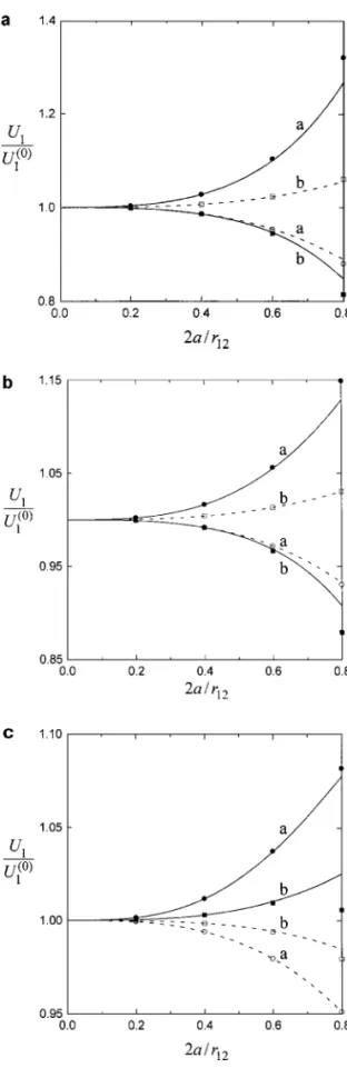
The exact (numerical) solution for the problem of diffusio-phoresis of two dielectric spheres parallel to the line through their centers was obtained by using a boundary collocation method (18). Figure 1 gives a comparison of our asymptotic results of the particle velocities (normalized by their undis-turbed values given by Eq. [1.5]) calculated from the method of reflections (illustrated by curves) with this exact solution

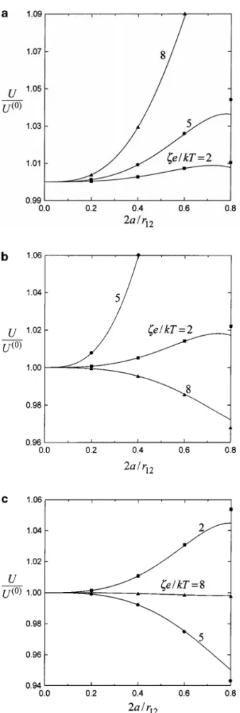
FIG. 1. Normalized diffusiophoretic velocities of two identical spheres with the line through their centers aligned with the imposed electrolyte gradient versus the separation parameter 2a/r12withζ e/kT as a parameter for the case of

f1= f2= 0.2 and κa = 100: (a) Z = 1; (b) Z = 2; (c) Z = 3. The points

represent the exact collocation solutions.

(shown by points). For simplicity, only the case of two iden-tical spheres (a1 = a2= a, ζ1= ζ2= ζ, U₁(0)= U₂(0) = U(0), where U(0)_j = U(0)_j d and d is the unit vector in the direction

of ∇n∞) with f1= f2= 0.2 and κa = 100 is presented. In the case of identical spheres, the particles will migrate at the same velocity (U1= U2= U, where Uj = Ujd). It is found in

Fig. 1 that the predictions of U/U(0) _{from the asymptotic} ap-proximation for various values of Z andζe/kT are in good agreement with those of the exact solution. The errors in diffu-siophoretic velocities are less than 0.28% for cases 2a/r12 ≤ 0.6 or 3.5% for cases 2a/r12≤ 0.8, indicating that the higher-order terms such as O(r₁₂−8) in Eq. [3.9] are not important unless the particles are nearly touching. For the cases of two spheres dif-fering in size and/or in zeta potential, or under the situation

f16= f2, Eq. [3.9a] can also be found to agree well with the exact solution.

The plots of the numerical values of Ui/U

(0)

i versus

para-metersζe/kT and κaifor various cases of two charged spheres

undergoing diffusiophoresis along the line through their centers were presented by Keh and Luo (18). Readers are suggested to refer to their work for details of the particle interactions in this axisymmetric configuration. The translational and rota-tional velocities for various cases of two identical spheres (with

Ä1= −Ä2 = Ä, where Ωj = Äje× d) undergoing

diffusio-phoresis perpendicular to the line through their centers evalu-ated from Eq. [3.9] are shown in Figs. 2–6. For the asymmetric configuration, there is no numerical solution available in the lit-erature to make a comparison. In Figs. 2 and 3 (for cases of

f1= f2and f16= f2, respectively), the velocities of a particle normalized by the value that prevails in the absence of the other are plotted versus the separation parameter 2a/r12for various values of Z andζe/kT . It can be seen that the effect of particle interactions on the normalized diffusiophoretic velocities is in-creased with the increase in 2a/r12. However, each sphere can be speeded up or slowed down (and rotated in either direction) by the movement of the other with the decrease of the separation distance, depending on the values of the relevant factors. In gen-eral, if the translational velocities of the two spheres undergoing diffusiophoresis normal to their line of centers are enhanced (or reduced) by the proximity of each other, then the angular veloc-ityÄ (and diffusiophoretic velocities along their line of centers, which are shown in Fig. 1) will be decreased (or increased). For some typical cases, the effect of particle interactions can be quite significant as the particles get close to each other. Note that the situations associated with Figs. 2a and 3a are close to those of diffusiophoresis in the aqueous solutions of KCl and NaCl, respectively.

The normalized diffusiophoretic velocities of two identical spheres in the direction normal to the line through their centers are plotted as a function of their dimensionless zeta potential at different values ofκa (20, 100, and ∞) and Z in Fig. 4 for a case in which the cation and anion mobilities are equal (with

f1= f2= 0.2 and 2a/r12= 0.6). Only the results at positive zeta potentials are displayed in this figure since, for D2= D1,

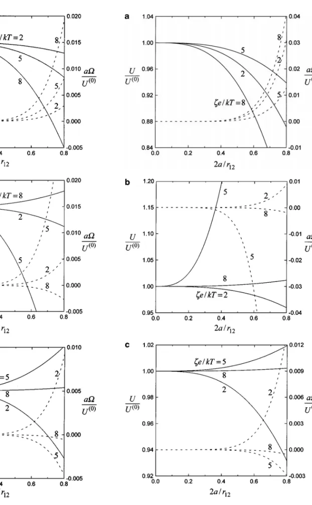
FIG. 2. Normalized translational (solid curves) and rotational (dashed curves) velocities of two identical spheres undergoing diffusiophoresis per-pendicular to the line through their centers versus the separation parameter 2a/r12withζe/kT as a parameter for the case of f1= f2= 0.2 and κa = 100:

(a) Z= 1; (b) Z = 2; (c) Z = 3.

FIG. 3. Normalized translational (solid curves) and rotational (dashed curves) velocities of two identical spheres undergoing diffusiophoresis perpen-dicular to the line through their centers versus the separation parameter 2a/r12

withζ e/kT as a parameter for the case of (D2− D1)/(D2+ D1)= −0.2, f1=

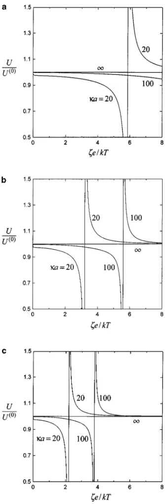
FIG. 4. Normalized translational velocities of two identical spheres under-going diffusiophoresis perpendicular to the line through their centers versus the dimensionless zeta potentialζe/kT with κa as a parameter for the case of

f1= f2= 0.2 and 2a/r12= 0.6: (a) Z = 1; (b) Z = 2; (c) Z = 3.

the induced macroscopic electric field vanishes and the parti-cle velocities, which are due to the chemiphoretic effect only, will be an even function of the zeta potential. When the value of Z eζ/kT is small (say, <6), the normalized diffusiophoretic mobility of each particle is a monotonic decreasing function of

Z eζ/kT for a finite value of κa. Also, this mobility is smaller

with smallerκa. However, when the value of Zeζ/kT is in-creased, a minimum and a maximum of the normalized mobil-ity would appear. As Z increases orκa decreases, the extremes occur at smaller zeta potentials. Note that the abrupt variation of the normalized particle velocity near these extremes is due to the fact that the direction of the undisturbed velocity U(0) re-verses and its magnitude is small over there (refer to Refs. 3 and 11), while the interacted particle velocity Uj does not reverse

synchronously.

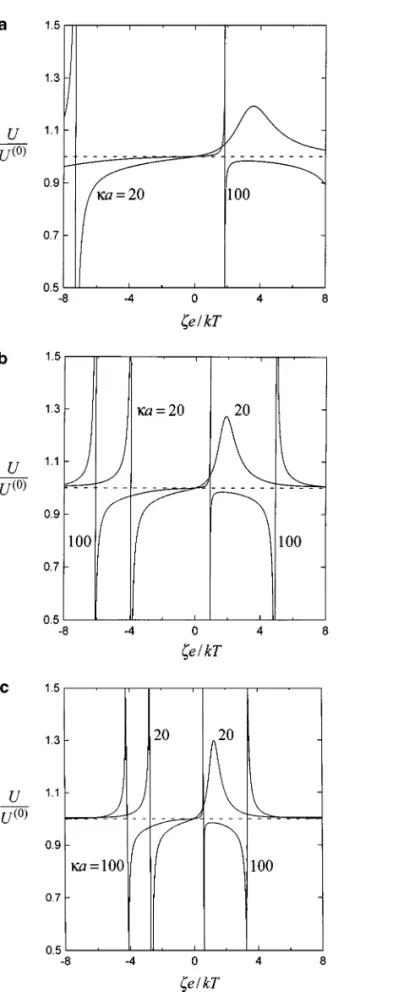
The normalized diffusiophoretic velocities of two identical spheres perpendicular to their line of centers as a function of

ζ e/kT at different valus of κa and Z for a case in which the

cation and anion have different diffusion coefficients [(D2−

D1)/(D2+ D1)= −0.2 with f1= 0.2 and 2a/r12 = 0.6] are depicted in Fig. 5. In this case, both the chemiphoretic and the electrophoretic effects contribute to the particles’ movement and the net diffusiophoretic velocities are neither an even nor an odd function ofζ. It can be seen that the normalized diffusio-phoretic mobility of each sphere is not a monotonic function of

ζ e/kT . In general, no simple rule could appropriately describe

the particle interactions. Whether the diffusiophoretic mobil-ity is increased or decreased depends on the combination of

ζ e/kT, κa, Z, f1, and f2. Since the undisturbed particle veloc-ity U(0)_{in the given range ofζe/kT (from −8 to 8) can reverse its} direction more times in diffusiophoresis with D26= D1than in pure chemiphoresis, there are more extremes of the normalized particle mobility in Fig. 5 than in Fig. 4.

In Fig. 6, the diffusiophoretic velocities of two identical spheres normal to their line of centers are plotted versus κa in the range from 20 to 105_{for a case of D}

2= D1. It is shown that there will be no particle interaction in diffusiophoresis as long as the value ofκa approaches infinity (the diffusiophoretic mobilities of the particles will be equal to the value calculated by Eq. [1.2] ignoring the polarization effect of the double layer). For the case Z = 1, the particle interaction in general is weak-ened steadily asκa becomes large gradually. However, when the value of Z eζ/kT gets large (say, >6), there can be a min-imum and a maxmin-imum of the particle interaction occurring at some value ofκa for a given value of ζe/kT . If the particles are charged more highly (with greater magnitude in zeta poten-tial) or the counterions have a larger absolute value of valence, the locations of these maximal particle interactions will shift toward largeκa; that means larger values of κa are required to make the assumption ofκa → ∞ valid. This behavior is in accordance with the limiting requirement given by Eq. [1.4]. Al-though only the situation of D2 = D1is displayed in Fig. 6, the plot of U/U(0)versusκa for cases with D26= D1will indicate a similar outcome.

FIG. 5. Normalized translational velocities of two identical spheres un-dergoing diffusiophoresis perpendicular to the line through their centers ver-sus the dimensionless zeta potentialζe/kT with κa as a parameter for the case of (D2− D1)/(D2+ D1)= −0.2, f1= 0.2, and 2a/r12= 0.6: (a) Z = 1;

(b) Z= 2; (c) Z = 3.

FIG. 6. Normalized translational velocities of two identical spheres under-going diffusiophoresis perpendicular to the line through their centers versusκa withζe/kT as a parameter for the case of f1= f2= 0.2 and 2a/r12= 0.6:

5. MEAN DIFFUSIOPHORETIC VELOCITY IN BOUNDED SUSPENSIONS

The interaction effects between pairs of arbitrarily oriented particles undergoing diffusiophoresis, obtained in Section 3, can be extended to the evaluation of the average diffusiophoretic velocity in a suspension of charged sphers. In the following, formulas for this average velocity correct to the order of first power of the volume fraction of the particles will be derived.

For a bounded suspension of particles subjected to an imposed electrolyte concentration gradient∇n∞, it is no longer possible to define the particle velocity relative to the distant fluid. Instead, the particle velocity should be calculated for a reference frame in which the net particle and fluid flux is zero and∇µ∞_m defined by Eq. [3.4] are the volume average of the electrochemical potential gradient fields over the entire suspension. Thus,

1 V Z V v(x) dx= 0, [5.1a] 1 V Z V ∇µm(x) dx= ∇µ∞m, [5.1b]

where V denotes the entire volume of the suspension.

On the basis of a microscopic model of particle interac-tions in a dilute dispersion which involves both statistical and low Reynolds number hydrodynamic concepts (26, 27), the ensemble-averaged diffusiophoretic velocity of a “test” particle (denoted by the subscipt t) in a suspension of spherical particles subject to Eq. [5.1] can be expressed as

hUti = U (0) t + C ( Z V v∗(r)[g(r)− 1] dr + 2 X m₌₁ Z V (Gm)t[∇µ∗m(r)− ∇µ∞m][g(r)− 1] dr + Z V W(r)g(r) dr ) + O(C2_{). [5.2]}

Here, U(0)_t =P2_m=1(Gm)t∇µ∞m, which is the undisturbed

diffu-siophoretic velocity of the test particle in a symmetric electrolyte given by Eq. [2.28], g(r) is the radial distribution function de-scribing the two-particle configurational probability, and C is the macroscopic concentration of the neighbor particles (assumed to be identical with zeta potentialζ and radius a). ∇µ∗_m(r) and

v∗(r) are the electrochemical potential gradient and fluid veloc-ity fields, respectively, at position r, when a neighboring particle at the origin 0 moves due to the prescribed concentration gra-dient∇µ∞_m, which are expressed by Eq. [3.5] (eliminating the superscripts and subscripts) for r ≥ a. Inside the neighboring particle (r < a), both ∇µ∗_mand v∗are constant,

∇µ∗ m= ∇µ∞m + 2 X i₌₁ (gmi)∇µ∞i , [5.3a] v∗ = 2 X m₌₁ (Gm)∇µ∞m. [5.3b]

Note that Eq. [5.3a] gives only the assumed quantity for∇µ∗_m, which satisfies Laplace’s equation and the continuity at the parti-cle surface (r= a) for µ∗_m. W(r) is a correction function needed to account for the perturbation on v∗(r) owing to the presence of the test particle, and is given by

W(r)= U∗_t(r)− U(0)t − v∗(r)− 2 X m₌₁ (Gm)t £ ∇µ∗ m(r)− ∇µ∞m ¤ , [5.4] where U∗_t(r) is the actual velocity of the test particle located at

r with respect to the origin of a single neighboring particle at 0. U∗_t(r) can be calculated from the summation of Eqs. [3.3a] and [3.8a], taking subscripts 1 and 2 to denote the test and neighbor-ing particles, respectively. Note that the Faxen correction term involving∇2v∗, which should have appeared in Eqs. [5.2] and [5.4], equals zero, as computed from using Eq. [3.5b].

To evaluate the volume integrals in Eq. [5.2], we assume that the radial distribution function has the following equilibrium value for rigid spheres without long-range pair potential:

g= 0 if r < at+ a, [5.5a]

g= 1 + O(C) if r > at+ a, [5.5b]

where O(C) is a term proportional to the concentration of neigh-bors. In other words, the particles must be sufficiently small so that Brownian motion dominates any multiparticle hydrody-namic interactions that might impart microscopic structure to the suspension. In general, it is necessary to obtain the pair dis-tribution function as the solution of a conservation equation of Fokker–Planck type for a polydisperse system of spheres (28). The conditions under which the assumption of the local equilib-rium is valid for a dilute dispersion consisting of different types of particles are also discussed by Reed and Anderson (27).

Given Eq. [3.5] or [5.3] for∇µ∗_m(r) and v∗(r), combination of Eqs. [3.3a] and [3.8a] for U∗_t(r), Eq. [5.4] for W(r), and Eq. [5.5] for g(r), the integrals in Eq. [5.2] are evaluated to obtain

hUti = U (0) t [1+ αtϕ + O(ϕ2)], [5.6] with αt= 1 At ( −A − 2 2 X m₌₁ (Gm)t(bm)+ µ at at+ a ¶3 × " −2 2 X m=1 (Gm)(bm)t+ 4 2 X m=1 2 X i=1 (Gm)t(gmi)(bi)t − 12 2 X m=1 (Hm)(bm)t− 5 2At #) , [5.7]

whereϕ = 4πa3_{C/3 is the volume fraction of the neighbor} par-ticles. The three terms in the braces of Eq. [5.7] forαtare ob-tained in order of the contributions from the first, second, and third integrals in Eq. [5.2]. This result is not exact, even given Eq. [5.5] holds, because O(r₁₂−8) terms are neglected in U∗_t(r); the error will appear only in the calculation involving the correction function W(r). In the derivation of Eq. [5.7], all the neighbor particles were assumed to be identical, even though they are allowed to differ from the test particle.

For a dilute suspension of particles that have a distribution in radius and/or zeta potential, a generalization of Eqs. [5.6] and [5.7] yields hUki = U (0) k · 1+X l αklϕl+ O(ϕ2) ¸ , [5.8] αkl = 1 Ak ( −Al− 2 2 X m=1 (Gm)k(bm)l+ µ ak ak+ al ¶3 × " −2 2 X m=1 (Gm)l(bm)k+ 4 2 X m=1 2 X i=1 (Gm)k(gmi)l(bi)k − 12 2 X m=1 (Hm)l(bm)k− 5 2Ak #) . [5.9]

Here,ϕ =P_lϕland the subscript k denotes the type of particles

having radius akand uniform zeta potentialζk.

In a suspension of identical particles, the expression for the average diffusiophoretic velocity can be reduced from Eqs. [5.8] and [5.9] to hUi = U(0)_{[1+ αϕ + O(ϕ}2_{)], [5.10]} α = 1 A " −A − 2 2 X m=1 Gmbm+ 1 8 Ã −2 2 X m=1 Gmbm + 4 2 X m=1 2 X i=1 Gmgmibi− 12 2 X m=1 Hmbm− 5 2A !# . [5.11]

In the limiting situation given by Eq. [1.4] (no polarization effect in the electric double layer surrounding each particle), Eqs. [5.9] and [5.11] giveαkl= α = −3/2 and the contribution from the

correction function W toα vanishes (irrespective to whether the suspension has a particle size distribution or not). The reason for a nonzero value ofα in this limit (where there is no inter-action between a pair of particles with the same zeta potential in an unbounded fluid) is that in the bounded suspension the volume-averaged flow is zero (this contributes−1 to α) and the volume-averaged electrochemical potential gradients are∇µ∞_m (this contributes−1/2 to α), as required by Eq. [5.1].

Results ofα calculated from Eq. [5.11] for a suspension of identical particles at different values ofκa and Z are plotted versusζ e/kT in Fig. 7a for a case of D2 = D1. It can be seen that the mean diffusiophoretic velocity is reduced with an increase

FIG. 7. Coefficientα evaluated from [5.11] for the diffusiophoresis of a suspension of identical spheres versusζe/kT : (a) f1= f2= 0.2, solid curves

represent the case Z= 1 and dashed curves denote the case Z = 2; (b) Z = 1, (D2− D1)/(D2+ D1)= −0.2 and f1= 0.2.

in the particle concentration (the value ofα is negative) in the range ofκa ≥ 100 and |ζ|e/kT ≤ 8 when Z = 1. On the other hand, for the representative situations ofκa = 20 when Z = 1 and ofκa = 100 when Z = 2 (or 3, which is not shown in this figure), the particle velocity can be enhanced with the increase of

ϕ (the value of α can be positive) in the considered range of zeta

potential and a maximum and a minimum ofα can appear. The abrupt variation ofα near these extremes is also due to the fact that the direction of the undisturbed velocity U(0) reverses and its magnitude is small over there. In Fig. 7b,α as a function of

ζ e/kT at two different values of κa for the case of Z = 1, (D2−

D1)/(D2+ D1)= −0.2, and f1 = 0.2 is illustrated. The results for the cases Z = 2 and 3 will give a similar dependence of α on ζ e/kT . Again, the value of α can be positive or negative depending on the relevant factors.

Figure 8 shows the calculations of α from Eq. [5.11] for monodisperse suspensions as a function ofκa over the range

FIG. 8. Coefficientα evaluated from [5.11] for the diffusiophoresis of a suspension of identical spheres versusκa for the cases of Z = 1 (solid curves) and Z= 2 (dashed curves) with f1= f2= 0.2.

20–105 _{for a case of D}

2= D1. As expected, α → −3/2 as κa → ∞ for various values of Z and ζ e/kT . For given

val-ues of Z andζ e/kT , there can be a maximum and a minimum ofα occurring at some κa and the value of α can be positive or negative. The plot ofα versus κa for cases with D2 6= D1will display a similar dependence as Fig. 8.

6. ELECTROPHORESIS IN A SYMMETRIC ELECTROLYTE

Considered in this section is the electrophoretic motions of a single charged sphere in an arbitrary electric field, of two charged spheres in a uniform electric field, and of a dilute suspension of charged spheres. The bulk concentration n∞of the symmetri-cally charged electrolyte beyond the electric double layers is constant. Like the analysis in the previous sections, the thick-ness of the double layers is assumed to be much smaller than the particles’ radii and the surface-to-surface distance between the neighboring particles, but the polarization effect in the thin diffuse layers is incorporated.

First we examine the motion of a single dielectric sphere of radius a with uniform zeta potentialζ in an arbitrary imposed electric field EA(x). Outside the double layer, the

electrochem-ical potentials of the ions satisfy Laplace’s equation [2.1] and boundary condition [2.4] at the particle surface, but the condition [2.8] at infinity is replaced by

r→ ∞: µm→ µm A= µ0m+ kT ln n∞− zmeEA· x. [6.1]

The solution for µm in this case can still be expressed as

Eq. [2.19]. The governing equations, boundary conditions, and solution for the velocity field have the same forms as those given in Section 2. The final result for the electrophoretic velocity of

the particle can be written as

U= Ae(EA)0, [6.2] where

Ae= εkT

3πηZe[(2+ c1+ c2) ¯ζ + (c1− c2) ln cosh ¯ζ], [6.3] instead of Eqs. [2.29] and [2.30] for the diffusiophoretic velocity. Analogous to the case of diffusiophoresis, this result is identical to Eq. [1.3] with EA evaluated at the position of the particle

center.

We now examine the motion of two dielectric spheres in a constant applied electric field E_∞. Similar to the case of motion of a single sphere, the formulas presented in Section 3 for the diffusiophoresis of two spheres are still valid for electrophoresis, except that condition [3.4] should be changed into

µ∞

m = µ

0

m+ kT ln n∞− zmeE∞· x, [6.4]

and the final result for the translational and angular velocities give by Eq. [3.9] is replaced by

U1 = Ae1E∞+ " 1 2A e 2+ Ze 2 X m=1 (−1)m(Gm)1(cm)2 #µ a2 r12 ¶3 × (3ee − I) · E∞+ ( Z e 2 X m=1 " 1 2(−1) m_(G m)2(cm)1 − 2 X i=1 (−1)m(Gm)1(gmi)2(ci)1 # (3ee+ I) + " 18Z e 2 X m=1 (−1)m(Hm)2(cm)1− 15 2 A e 1 # ee ) a3 1a 3 2 r₁₂6 · E∞ + O¡r₁₂−8¢, [6.5a] Ω1 = " −9Ze 2 X m=1 (−1)m(Hm)2(cm)1+ 15 4 A e 1 # a3₁a3₂ r7 12 e × E∞+ O¡r₁₂−9¢. [6.5b] In Eq. [6.5], the variables (gmi)j, (cm)j, (Gm)j, (Hm)j, and Aej

denote those defined by Eqs. [2.13], [2.15], [2.26], [2.27], and [6.3], respectively, for the particle j ( j = 1 or 2).

The exact (numerical) solution for the problem of elec-trophoresis of two arbitrary dielectric spheres with thin but polar-ized double layers was obtained by using the boundary collection method (10, 17). Figure 9 gives a comparison of our asymptotic results of the normalized electrophoretic velocity U1/U

(0) 1 cal-culated from Eqs. [6.5a] and [1.3] (illustrated by curves) for the case of two equal-sized spheres with f1 = f2 = 0.4 and κa = 100 with the exact solution (shown by points) and

FIG. 9. Normalized electrophoretic velocity U1/U1(0)versus the separation

parameter 2a/r12for the case of two spheres with a1= a2= a, f1= f2= 0.4,

andκa = 100: (a) Z = 1; (b) Z = 2; (c) Z = 3. The solid curves are plotted when the line through particle centers is parallel to the applied electric field, while the dashed curves are drawn when this line is perpendicular to the applied electric field. Curves “a” represent the cases withζ1e/kT = 1 and ζ2e/kT = 5;

curves “b” denote the cases withζ1e/kT = 5 and ζ2e/kT = −5. The points

represent the exact collocation solutions.

0.32% (or 0.07%) for cases 2a/r12≤ 0.6 and 4.3% (or 1.1%) for case 2a/r12 ≤ 0.8 when the two spheres are oriented parallel (or perpendicular) to the applied electric field E_∞. In the cases of two spheres having different radii, Eq. [6.5] can also be found to agree well with the exact solution. For most situations, the interaction between the two electrophoretic particles does not vary monotonically with the parametersζe/kT and κa. Simi-lar to the case of diffusiophoresis of two spheres discussed in Section 4, if the electrophoretic velocity of one sphere is en-hanced (or reduced) by the other when the electric field is applied normal to the line through their centers, this velocity will be re-duced (or enhanced) when the electric field is imposed parallel to the line of particle centers.

Finally, we consider the electrophoretic motion of a suspen-sion of dielectric spheres. The analysis presented in Section 5 is also valid for this case, provided that Eq. [6.4] is used for

µ∞

m instead of Eq. [3.4] and U(0)represents the electrophoretic

velocity given by Eq. [1.3]. With these changes, the result forαt given by Eq. [4.7] becomes

αt = 1 Ae_t ( −Ae_{+ Ze} 2 X m=1 (−1)m(Gm)t(cm) + µ at at+ a ¶3" Z e 2 X m=1 (−1)m(Gm)(cm)t −2Ze 2 X m₌₁ 2 X i₌₁ (−1)i(Gm)t(gmi)(ci)t + 6Ze 2 X m=1 (−1)m(Hm)(cm)t− 5 2A e t #) . [6.6] The expression forαkl andα in Eqs. [5.9] and [5.11] for

poly-disperse and monopoly-disperse suspensions, respectively, should be altered accordingly. Analogous to the corresponding case of dif-fusiophoresis, Eq. [6.6] givesαt= αkl= α = −3/2 for a

suspen-sion of particles having the same zeta potential in the limiting situation given by Eq. [1.4]. Note that the use of the analytical formula [6.5] to evaluateαthas a great advantage over the use of the numerical solutions for the interaction between two elec-trophoretic spheres in that a complicated numerical integration (which usually leads to some errors, too) can be avoided in the calculation of Eq. [5.2].

Results of the coefficientα for the electrophoresis of a sus-pension of identical spheres with D2 = D1 at various values of Z, ζ e/kT , and κa calculated using Eq. [6.6] are shown in Fig. 10. Only the results at positive zeta potentials are shown sinceα is an even function of ζ here. It can be found in all cases that the average electrophoretic velocity always decreases with an increase in the particle concentration (with−3/2 ≤ α < 0) and the effect of interactions between two particles (in an un-bounded fluid) is to reduce the magnitude ofα. It can be seen that a maximum ofα can exist at some ζe/kT for a fixed value of κa and at someκa for a constant value of ζe/kT . When the value