數個應用於隱私保護資料探勘之啟發性方法

全文

(1)國立高雄大學資訊工程學系(研究所) 碩士論文. 數個應用於隱私保護資料探勘之啟發性方法 Several Heuristic Approaches to Privacy-Preserving Data Mining. 研究生：楊國棟指導教授：洪宗貝. 撰博士. 中華民國九十九年七月.

(2) 致謝經過這兩年研究所的學習經歷，對於這篇論文能順利完成，為這個生涯中燦爛的片段畫下美麗的句點，有太多的人需要感謝。首先我要感謝的是我的指導教授，洪宗貝博士。洪老師是當初鼓勵我繼續進修的推手，在論文構思的方向及研究的方法上總是給予許多建議；且在繁忙的行政工作與教學研究過程中，老師還不時撥空為學生的論文做指導與修改。除此之外，亦師亦友的互動過程中，老師平日待人處事的態度也深深的影響已有家庭且在職場工作的我，讓我獲益良多。同時，我要感謝我的碩士論文口試委員：李健興教授、林文揚教授及林葭華教授。謝謝你們撥空來參加我的碩士論文口試，並且對於我的碩士論文的內容給予寶貴的建議及指導，使本論文更臻完善。其次，我要感謝實驗室的伙伴：浚瑋學長、國誠學長、明泰學長、韋體學長、欣怡學姐、偉屏、廷一、宗慶、世濱、峰世、柏諺。感謝你們在這些日子的互相砥礪與照顧。尤其是浚瑋學長對我論文的修正花了很大的心力，謝謝你。我還要感謝辦公室的工作同仁：趙兄、則明與世澤。感謝你們容忍我這兩年來在工作上的怠惰，並分擔我分內應要處理的業務，使得我在工作期間得以偷閒專心在課業上。沒有這樣的優勢，相信在兩年內我是無法完成研究所課業的。你們的這份恩情，我謹記在心。最後也是最重要的，我必須要感謝我親愛的老婆瑋琪，這些日子妳默默地承擔起照顧我那一對可愛稚子的責任，並且家中大部分的家務皆由妳一個人操持。沒有妳無悔的付出與支持，沒有妳無私的犧牲與無微不至的照顧，我絕無這樣的環境與毅力能夠安心地完成研究所學業。這種感動與感激不是三言兩語能夠訴說完的。老婆，我愛妳。謹誌於知識工程與人工智慧實驗室/高雄大學圖書資訊館楊國棟. i. 2010.08.09.

(3) 數個應用於隱私保護資料探勘之啟發性方法. 指導教授：洪宗貝博士（教授）國立高雄大學資訊工程所. 學生：楊國棟國立高雄大學資訊工程所. 摘要資料探勘的技術可以協助人們從大量的數據中獲取有用的知識，但是在資料收集與數據傳播的過程當中，可能因某些因素導致敏感及隱私的資料受到外洩威脅的風險。所以，有關個人、企業和組織敏感的資訊，應在公布之前即被受限、制止或保護，也因此近幾年，處理隱私保護之資料探勘成為一個重要的研究議題。在本篇論文中，我們提出三種方法藉由修改原始的資料庫，達到隱藏敏感項目集的目的。第一個方法稱為 SIF-IDF，它是一個以貪婪演算法為基礎的方法，其主要的想法是借用在文件探勘上利用詞頻與逆向文件頻率 (TF-IDF)作關鍵字分析的技巧來評估交易項目集與敏感項目集間的相似程度，然後在一些交易中選擇適當的項目來隱藏。第二個方法是以晶格為基礎的方法，晶格的構建是基於以敏感資料集間關係的分類結果。此外，我們也使用由下而上的刪除策略來逐步減少敏感資料集頻率，以快速達成敏感資料隱藏的目的。最後第三個方法是一個演化式的隱私保護資料探勘的方法，用以從資料庫中尋找最適合的交易進行隱藏。此方法使用了三個變數來設計一個靈活的評估函數，並且可根據使用者的愛好彈性地分配此三變數的權重。除此之外，準大項目集的概念也被應用來減少重新掃描資料庫的成本，加快評估染色體的過程。此三個方法可在隱私保護與執行時間中取得一好的折衷平衡，而實驗結果也顯示所提方法在效能上有優越的表現。關鍵字：隱私保護、資料探勘、晶格、基因演算法、準大項目集. ii.

(4) Several Heuristic Approaches to Privacy-Preserving Data Mining Advisor: Dr. (Professor) Tzung-Pei Hong Department of Computer Science and Information Engineering National University of Kaohsiung. Student: Kuo-Tung Yang Department of Computer Science and Information Engineering National University of Kaohsiung. ABSTRACT Data mining technology can help extract useful knowledge from large data sets. The process of data collection and data dissemination may, however, result in an inherent risk of privacy threats. Some sensitive or private information about individuals, businesses and organizations needs to be suppressed before it is shared or published. The privacy-preserving data mining (PPDM) has thus become an important issue in recent years. In this thesis, we propose three approaches for modifying original databases in order to hide sensitive itemsets. The first one is called SIF-IDF, which is a greedy approach based on the concept borrowed from the Term Frequency and Inverse Document Frequency (TF-IDF) in text mining. It uses the above concept to evaluate the similarity degrees between the items in transactions and the desired sensitive itemsets and then selects appropriate items in some transactions to hide. The second one is a lattice-based approach, in which a lattice is built based on the relation of sensitive itemsets. The bottom-up deletion strategies is also used to gradually reduce the frequency of sensitive itemsets in the hiding process. The third one is an evolutionary privacy-preserving data mining method to find appropriate transactions to be hidden from a database. The proposed approach designs a flexible evaluation function with three factors, and different weights may be assigned to them depending on users’ preference. Besides, the concept of pre-large itemsets is used to reduce the iii.

(5) cost of rescanning databases, thus speeding up the evaluation process of chromosomes. The three proposed approaches can easily make good trade-offs between privacy preserving and execution time. Experimental results also show the performance of the proposed approaches.. Keywords: Privacy preserving, Data mining, Lattice, Genetic algorithm, Pre-large itemsets. iv.

(6) Contents 致謝....................................................................................................................................... i 摘要..................................................................................................................................... iii ABSTRACT ....................................................................................................................... iv List of Figures .................................................................................................................... ix List of Tables ...................................................................................................................... xi Chapter 1. Introduction ............................................................................................... 1. 1.1. Motivation ................................................................................................. 1. 1.2. Contributions ............................................................................................. 3. 1.3. Thesis Organization................................................................................... 4. Chapter 2. Related Works ........................................................................................... 5. 2.1. Data Mining Process.................................................................................. 5. 2.2. Data Sanitization ....................................................................................... 6. 2.3. Genetic Algorithms ................................................................................... 7. 2.4. The Concept of Pre-Large Itemsets........................................................... 8. Chapter 3. Problem Formulation............................................................................... 11. Chapter 4. A Greedy Approach Based on Sensitive Items Frequency and Inverse Database Frequency................................................................................. 14. 4.1. The Proposed SIF-IDF Algorithm........................................................... 16. 4.2. An Example ............................................................................................. 18. Chapter 5. A Greedy Approach Based on Lattices ................................................... 26. 5.1. The Proposed Lattice-Like Algorithm..................................................... 30. 5.2. An Example ............................................................................................. 31. Chapter 6 6.1. A GA-Based Approach for PPDM .......................................................... 40 Chromosome Representation................................................................... 40 v.

(7) 6.2. Fitness Function ...................................................................................... 41. 6.3. Genetic Operators.................................................................................... 45 6.3.1 Crossover................................................................................................. 45 6.3.2 Mutation .................................................................................................. 46 6.3.3 Selection .................................................................................................. 47. 6.4. The Proposed GA-based Algorithm for PPDM....................................... 48. 6.5. An Example ............................................................................................. 50. Chapter 7. Experimental Results............................................................................... 55. 7.1. Experimental Results of SIF-IDF Algorithm .......................................... 55. 7.2. Experimental Results of Lattice-Like Algorithm .................................... 58. 7.3. Experimental Results of GA-based Algorithm........................................ 61. Chapter 8. Conclusion and Future Work................................................................... 65. References. ................................................................................................................. 67. vi.

(8) List of Figures Figure 2-1: Nine cases for candidate itemsets due to record deletion............................9 Figure 3-1: Two kinds of removal ................................................................................12 Figure 4-1: The flowchart of SIF-IDF algorithm..........................................................16 Figure 5-1: A lattice structure with five items ..............................................................26 Figure 5-2: The lattice structure built from the three sensitive itemsets.......................27 Figure 5-3: The flowchart of the proposed lattice-like approach .................................29 Figure 5-4: The lattice structure after complete the combination procedure in 2-level 34 Figure 5-5: The lattice structure after complete the combination procedure................35 Figure 5-6: The deletion process of items {acfh} in S123 ...........................................36 Figure 5-7: The deletion process of set S12..................................................................37 Figure 5-8: The deletion process of item {c} in set of S3 ............................................39 Figure 6-1: An example for a chromosome ..................................................................40 Figure 6-2: The relationship of itemsets before and after the PPDM process ..............41 Figure 6-3: The set of sensitive itemsets that fail to be hidden ....................................42 Figure 6-4: The set of missing itemsets ........................................................................43 Figure 6-5: The set of artificial itemsets .......................................................................44 Figure 6-6: The crossover operator...............................................................................46 Figure 6-7: The mutation operation ..............................................................................46 vii.

(9) Figure 6-8: The selection mechanism ...........................................................................47 Figure 6-9: The flowchart of the GA-based approach for PPDM ................................48 Figure 6-10: The large itemsets after the four transactions are deleted........................53 Figure 7-1: The relationships between EC value and the number of iterations in BMS-POS database with SIF-IDF approach.............................................56 Figure 7-2: The relationships between EC values and he number of iterations in BMS-Webview-1 database with SIF-IDF approach..................................57 Figure 7-3: The relationships between EC values and the number of iterations in BMS-Webview-2 database with SIF-IDF approach..................................57 Figure 7-4: The relationships between EC value and he number of iterations in BMS_POS database with lattice-like approach.........................................59 Figure 7-5: The relationships between EC value and he number of iterations in BMS-Webview-1 database with lattice-like approach ..............................59 Figure 7-6: The relationships between EC value and he number of iterations in BMS-Webview-2 database with lattice-like approach ..............................60 Figure 7-7: The relation between fitness and generation in BMS-POS database with GA-based approach ...................................................................................62 Figure 7-8: The relation between fitness and generation in BMS-WebView-1 database with GA-based approach ...........................................................................62 Figure 7-9: The relation between fitness and generation in BMS-WebView-2 database with GA-based approach ...........................................................................63 Figure 7-10: The relations between execution time and different database .................63. viii.

(10) List of Tables Table 4-1: A database example with 10 transactions.................................................. 19 Table 4-2: The SIF values of each sensitive itemset in each transaction.................... 20 Table 4-3: The MRC values of all the items............................................................... 21 Table 4-4: The IDF value of each item....................................................................... 21 Table 4-5: The IDF value of each sensitive itemset in each transaction .................... 22 Table 4-6: The SIF-IDF values for all the transactions .............................................. 23 Table 4-7: The sorted transactions according to the SIF-IDF values ......................... 24 Table 4-8: The result of the final sanitized database in the example.......................... 25 Table 5-1: An original database with 10 transactions................................................. 32 Table 5-2: The corresponding transactions of three sets ............................................ 33 Table 5-3: The corresponding transactions of the all sets in lattice structures ........... 34 Table 5-4: The output result of sanitized database with lattice-like approach ........... 39 Table 6-1: The set of the original database in the example ........................................ 50 Table 6-2: Large 1-itemsets ........................................................................................ 51 Table 6-3: Large 2-itemsets ........................................................................................ 51 Table 6-4: Large 3-itemsets ........................................................................................ 51 Table 6-5: Pre-Large 1-itemsets.................................................................................. 52 Table 6-6: Pre-Large 2-itemsets.................................................................................. 52. ix.

(11) Table 6-7: Pre-Large 3-itemsets.................................................................................. 52 Table 7-1: The details of the three databases.............................................................. 55 Table 7-2: The side effects of SIF-IDF algorithm ...................................................... 58 Table 7-3: The side effects of lattice-like algorithm................................................... 60 Table 7-4: The execution times of the proposed algorithms....................................... 61. x.

(12) Chapter 1 Introduction. 1.1. Motivation. In recent years, the privacy-preserving data mining (PPDM) has become an important issue due to the quick proliferation of electronic data in governments, corporations and non-profit organizations. Such data may implicitly contain confidential information and lead to privacy threats if they are misused. As the data mining technology rapidly progresses, getting users’ privacy information through data mining technology has become easier. Privacy information includes some confidential information, such as social security numbers, address information, credit card numbers, credit ratings and customer purchasing behavior, among others. Besides, the range of privacy information may be extended to businesses as well. Based on business purposes, some shard information among companies may be extracted and analyzed by other partners, which may not only increase the benefits of the companies but also cause threats to sensitive data. This has led to increasing concerns about the privacy of the underlying data and the implicit knowledge on the data. Verykios et al. [23] thus proposed a data sanitization process to hide sensitive knowledge by item addition or deletion. Their main concept was to reduce the supports of sensitive items such that the sensitive knowledge including the items might not be exposed. They also demonstrated that the problem was NP-hard. Since then, many techniques have then been proposed to modify or transform data such that the data privacy can be preserved. For example, Agrawal and Srikant. 1.

(13) proposed the k-anonymity [4] method for achieving the purpose of preserving privacy information. Each transaction in a public database was changed to have the same sensitive column values as at least (k-1) other transactions. Although the k-anonymity technology could successfully inhibit sensitive information, an appropriate balance between privacy and knowledge might not be guaranteed. Zhu et al. [24] then discussed what kind of public information type was suitable for not revealing sensitive data and insinuated that the k-anonymity technique might still have security problems. Verykios et al. [22] generally classified the privacy issues into two categories, which were data hiding and knowledge hiding. Data hiding concerned protection of underlying private data, but knowledge hiding focused on preserving high-level knowledge. In text mining, the technique of term frequency–inverse document frequency (TF-IDF) [21] is usually used to evaluate how relevant a word in a corpus is to a document. It may be thought of as a statistical measure. The importance of a word to a document depends on its appearing number in the document, but is offset by the frequencies of the words in the other documents. The first proposed approach in this thesis thus uses the concept and modifies the TF-IDF [21] to evaluate the degrees of transactions associated with given sensitive itemsets. It is a novel greedy-based approach, called sensitive items frequency - inverse database frequency (SIF-IDF), and is designed to reduce the frequencies of sensitive itemsets for data sanitization. Based on the SIF-IDF algorithm, the user-specific sensitive itmesets can be completely hidden with reduced side effects. In the SIF-IDF algorithm, the process for selecting hidden items is repeatedly executed for achieving the desired condition, thus requiring some amount of computational time. Thus another approach based on the lattice concept is proposed in this thesis to reduce the computational time. The second approach designs a lattice structure to efficiently sanitize a 2.

(14) database. Based on the downward closure property of the Apriori algorithm [5], each transaction classification set in the lattice structure can be efficiently checked to delete the items contained in sensitive itemsets. Recently, genetic algorithms (GAs) [11] have become increasingly important for researchers in solving difficult problems since they could provide feasible solutions in a limited amount of time. They are adaptive heuristic search algorithms derived from the evolutionary ideas of natural selection and genetics. As to using GAs to PPDM, Dehkordi [8] proposed an approach which encoded each transaction as a chromosome. The operators of selection, crossover and mutation were then used to adjust the population with a goal to hide sensitive itemsets. The performance of the approach might, however, greatly depend on the number of transactions in a database. In the third part of the thesis, a new GA-based PPDM approach is then proposed to conquer the problem. The proposed approach designs a flexible evaluation function with three factors, and different weights may be assigned to them depending on users’ preference. The proposed approach also adopts the concept of pre-large itemsets to avoid rescanning databases in chromosome evaluation. The efficiency can thus be greatly improved. The three proposed approaches can thus easily make good trade-offs between privacy preserving and execution time. Experimental results also show the performance of the proposed approaches.. 1.2. Contributions. This section states the contributions of this thesis, which can be divided into the three parts as follows.. 3.

(15) 1.. We propose a greedy-based approach called sensitive items frequency - inverse database frequency (SIF-IDF) for sanitizing databases in privacy-preserving data mining (PPDM). The proposed algorithm can effectively find appropriate transactions and modify them for hiding sensitive itemsets with reduced side effects.. 2.. We propose a lattice-like approach and designed a lattice structure to speed up the first approach for data sanitization. Based on the downward closure property of the Apriori algorithm, multiple transactions with the same sensitive itemsets can be symmetrically processed to save computational cost.. 3.. We propose a GA-based approach and design a flexible evaluation function with three factors, which are number of sensitive itemsets that fail to be hidden, number of the missing itemsets, and number of artificial itemsets. Each factor is attached a weight and can be flexibly specified by users. The concept of pre-large itemsets is also used to avoid the re-scan of databases for accelerating the evaluation process.. 1.3. Thesis Organization. The rest parts of this thesis are organized as follows. Some related works are described in Chapter 2. The problem to be solved in this thesis is described in Chapter 3. The first proposed SIF-IDF algorithm is stated in Chapter 4. The second proposed lattice-like approach is expressed in Chapter 5. The third proposed GA-based algorithm is explained in Chapter 6. Experimental results are then shown in Chapter 7. Conclusion and future works are given in Chapter 8.. 4.

(16) Chapter 2 Related Works In this chapter, we review some related researches about this thesis. Section 2.1 describes the data mining process. Section 2.2 introduces the general concept of data sanitization, which can be further classified as anonymity, blocking and encryption. Section 2.3 reviews genetic algorithms for solving optimization problems. Section 2.4 states the pre-large concept, which is integrated with the GA process in this thesis to avoid re-scanning databases for hiding sensitive itemsets.. 2.1. Data Mining Process. Data mining is most commonly used in attempts to induce association rules from transaction data, such that the presence of certain items in a transaction will imply the presence of some other items. To achieve this purpose, Agrawal et al. proposed several mining algorithms based on the concept of large itemsets to find association rules in transaction data [3][5][6]. They divided the mining process into two phases. In the first phase, candidate itemsets were generated and counted by scanning the transaction data. If the count of an itemset appearing in the transactions was larger than a pre-defined threshold value (called the minimum support), the itemset was considered a large itemset. Itemsets containing only one item were processed first. Large itemsets containing only single items were then combined to form candidate itemsets containing two items. This process was repeated until all large itemset had been found. In the second phase, association rules were induced from the large itemsets found in the first phase. All. 5.

(17) possible association combinations for each large itemset were formed, and those with calculated confidence values larger than a predefined threshold (called the minimum confidence) were output as association rules.. 2.2. Data Sanitization Years of effort in data mining have produced a variety of efficient techniques, which have. also caused the problems of security and privacy threats [14]. The research of privacy-preserving data mining (PPDM) has thus become a critical issue. PPDM is usually performed to hide sensitive information. In the past, Atallah et al. first proposed the protection algorithm for data sanitization to avoid the inference of association rules [2]. It used addition and deletion procedures to modify databases for hiding sensitive information. Dasseni et al. then proposed a hiding algorithm based on the hamming-distance approach to reduce the confidence or support values of association rules [7]. Three heuristic hiding approaches were thus proposed to increase the supports of antecedent parts, to decrease the supports of consequent parts, and to decrease the support of either the antecedent or the consequent parts, respectively. When the supports or the confidences of sensitive association rules were below user-specific minimum support thresholds, they could thus be hidden. Oliveira and Za¨ıane [18] then introduced the multiple-rule hiding approach to efficiently hide sensitive itemsets. It required only two database scans no matter the number of sensitive itemsets. In the first database scan, the index file was created to efficiently find sensitive itemsets within transactions. Three algorithms called MinFIA, MaxFIA and IGA were then used in the second database scan to remove minimal individual items. Amiri then proposed three heuristic approaches to hide multiple sensitive rules [1]. The first approach was called Aggregate,. 6.

(18) which computed the union of the supporting transactions for all sensitive itemsets and expelled the transaction that supports the most sensitive and the least non-sensitive itemsets. The second one was called Disaggregate, which aimed at removing individual items from transactions, rather than removing whole transactions. The third approach, called Hybrid, was a combination of the previous two. It uses the Aggregate approach to identify sensitive transactions and adopts the Disaggregate approach to selectively delete items from these transactions, until the sensitive knowledge has been hidden. Pontikakis et al. [19] then proposed two heuristics approaches based on data distortion. The first approach named priority-based distortion algorithm (PDA) was designed to reduce the confidences of sensitive rules by trying to decrease consequent items. The second approach called weight-based sorting distortion algorithm (WDA) was then proposed to prioritize selection of sanitized transactions. It used the priority values to weight the transactions based on effective data structures. The optimal sanitization of databases is, in general, regard as an NP-hard problem. Atallah et al. [2] proved that selecting which data to modify or sanitize was also NP-hard. Their proof was based on the reduction from the NP-hard problem of hitting-sets [9]. The hitting-set problem was first proven NP-hard. The PPDM problem was then reduced to the hitting-set problem in polynomial time. In this case, the PPDM problem could be said an NP-hard problem as well and could not be solved in polynomial time for now. That paper provided a solid theoretical background to explain that PPDM was a difficult issue.. 2.3. Genetic Algorithms Since 1960s, there has been much interest in developing powerful heuristic algorithms for. difficult optimization problems. Some nature-inspired approaches were then proposed to achieve. 7.

(19) the purpose. One of the most commonly used among them is the evolutionary computation based on Darwin theory: “Nature selects, the fittest survives”. In 1975, Holland [11] applied the concept of evolution into the field of dynamic algorithms and proposed genetic algorithms (GAs). Since then, GAs has become increasingly important for researchers in solving difficult problems because they could provide feasible solutions in a limited amount of time [10]. GAs have been successfully applied to the fields of optimization [15][16], machine learning [16], neural networks [20], fuzzy logic controllers [20], and so on. According to the principle of survival of the fittest, GAs generate the next population by several operations, with each individual in the population representing a possible solution. In general, a genetic algorithm has the following five basic components, as summarized by Michalewicz [17]: 1. A genetic representation of solutions to the problem, 2. A way for generating the initial population, 3. An evaluation function for measuring goodness of solutions, 4. Several genetic operators that alter the genetic composition of children, and 5. Parameter values.. 2.4. The Concept of Pre-Large Itemsets Hong and Wang proposed the pre-large itemsets [12] for efficient incremental data mining.. A pre-large itemset was not truly large (frequent), but might easily become large in the future through the data insertion process. Formally, a lower support threshold and an upper support threshold were used to realize this concept. The upper support threshold was the same as that in the conventional mining algorithms. The count of an itemset needed to be larger than the upper. 8.

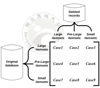
(20) support threshold in order to be regarded as large. The lower support threshold defined the lowest count for an itemset to be pre-large. Pre-large itemsets acted like a buffer in the incremental mining process and were used to reduce the movement of an itemset directly from large to small and vice verse. The concept of pre-large itemsets could also be used for record deletion [13]. In this thesis, we will delete transactions for PPDM. The processing for record deletion will thus be used and is explained below. When some records are deleted from a database, there are nine cases for candidate-itemsets to be considered, which are shown in Figure 2-1 [12].. Deleted records. Large Pre-Large Small itemsets itemsets itemsets. Original database. Large itemsets. Case1. Case2. Case3. Pre-Large itemsets. Case4. Case5. Case6. Small itemsets. Case7. Case8. Case9. Figure 2-1: Nine cases for candidate itemsets due to record deletion. In Figure 1, Cases 2, 3, 4, 7 and 8 do not affect the final association rules. Case 1 may remove existing association rules, and cases 5, 6 and 9 may generate new association rules. If we pre-store all large and pre-large itemsets from the original database, then Cases 1, 5 and 6 can be easily handled. Besides, an itemset in Case 9 cannot possibly be large for the entire updated. 9.

(21) database as long as the number of deleted records is a considerably small proportion of the original database. Hong and Wang derived the following theorem for Case 9 [15]. Given a lower support threshold Sl, an upper support threshold Su, and a transaction number d in a database, if the number f of deleted records satisfies the following condition, then an itemset in Case 9 (neither large nor pre-large in both the original database and in the deleted records) is not certainly large for the updated database: ⎢ ( S − Sl ) d ⎥ f ≤⎢ u ⎥ Su ⎣ ⎦. (1). Thus, no database rescan is needed if the above formula is satisfied. We may re-formulate the above formula and derive the following lower support threshold when the number f of deleted records for not rescanning databases is given:. f ⎞ ⎛ S l = S u × ⎜1 − ⎟ ⎝ d⎠. (2). The above formula will be used in the proposed GA-based PPDM approach to set an appropriate lower-bound threshold for efficient chromosome evaluation.. 10.

(22) Chapter 3 Problem Formulation In the problem of PPDM, some basic concepts are borrowed from association rule mining. Thus before exploring the PPDM’s issue, we need to know the definition of association rule mining. Agrawal extended and formalized the problem as follows [3]. Let I = {i1, i2, …, im} be a set of literals, called items. Let D be a set of transactions, where each transaction T ∈ D consists of a set of items, such that T ⊆ I. Each transaction T has a unique identifier, called its TID. A set of items X ⊂ I is called an itemset. An association rule is an implication of the form X ⇒ Y, where X ⊂ I, Y ⊂ I and X ∩ Y = ∅ . Usually, Y consists of only a single item. We say an association rule X ⇒ Y holds in a database D if the following two factors are satisfied. The first one is the support condition, which is defined as at least s% of the transactions in D contain X ∪ Y . It can be thought of as a measure of the frequency of a rule, and is expressed by. X ∪Y N. ≥ s , where N is the number of transactions in D. The second factor is the confidence. condition, which is defined as at least c% of transactions with the itemset X also contain Y. It is thus a measure of the strength of the rule, and is expressed by. X ∪Y X. ≥ c.. In privacy-preserving data mining, users may pre-specify a set of sensitive itemsets H = {{h1}, {h2}, …, {hi}}, which may be mined out from a database but is sensitive. We aim at preventing these sensitive itemsets being disclosed, and a solution is to reduce the frequencies of the sensitive itemsets from D. Let the modified database be denoted D’. Thus, each sensitive itemset will not have enough support to be frequent in D’. This kind of approaches can be thought of as support-based ones, and have to satisfy the constraint of |hi|/N’ < s, where N’ is the. 11.

(23) number of transactions in D’ and |hi| is number of occurrences of the sensitive itemset hi. In addition to hiding the sensitive itemsets from being mined, some other goals have been set as well when the original database is sanitized. For example, all of the non-sensitive rules should be successfully mined from the sanitized database D’. Besides, the rules that are not found in the original database D should not be generated from the sanitized database D’. In this thesis, we would like to hide sensitive itemsets, which are predefined by users. For achieving this purpose, new items or transactions may be inserted, or old items or transactions may be deleted or modified. Here, we will only focus on the deletion of items or transactions for PPDM. We use the data sanitization process to hide sensitive knowledge by item or transaction deletion that reduces the support of the rules below the user specified security threshold. Two kinds of removal are considered. One is removing items from transactions and the other is removing transactions from databases. An example for the two kinds of removal is shown in Figure 3-1. At the left of Figure 3-1, an item is removed, and at the right, a whole transaction is deleted.. Figure 3-1: Two kinds of removal. 12.

(24) In this thesis, three approaches are proposed for PPDM. The first two are called the sensitive items frequency - inverse database frequency (SIF-IDF) approach and the lattice-like approach, which are designed for removing items from transactions for hiding sensitive Itemsets. The third one is a GA-based approach, which delete transactions from a database for PPDM.. 13.

(25) Chapter 4 A Greedy Approach Based on Sensitive Items Frequency and Inverse Database Frequency. In this chapter, a greedy-based approach called sensitive items frequency - inverse database frequency (SIF-IDF) is proposed to hide given sensitive itemsets. It uses and modifies the. concept of TF-IDF [21] in text mining to evaluate the degrees of transactions associated with given sensitive itemsets. The measure for the SIF-IDF value of a transaction Ti is defined as follows: p ⎛ siij n ⎜ SIF − IDF (Ti ) = ∑ × ∑ log ⎜ Ti k =1 f k − MRCk j =1 ⎝ n. ⎞ ⎟, ⎟ ⎠. (3). where siij is the number of sensitive items contained in the j-th sensitive itemset in Ti, and Ti is the number of items in transaction Ti, n is the number of records in a database, f k is the frequency count of each item, and MRCk is the maximum reduced count of each item. The above formula consists of two components. One is the sensitive items frequency (SIF) and the other is the inverse database frequency (IDF). The sensitive items frequency (SIF) value is measured for each sensitive itemset sij in a transaction Ti. It is calculated as the number (|siij|) of sensitive items in Ti which are included in an assigned sensitive itemset sij divided by the number of all the items in Ti. On the contrary, the inverse database frequency (IDF) value shows the influence degree of the sensitive itemsets within a transaction by considering the whole database. In this chapter, the SIF-IDF value of each transaction is calculated and is used to 14.

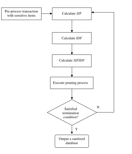
(26) measure whether a transaction has a large number of sensitive items but with less influence to other transactions. The transactions with high SIF-IDF values are considered to be processed with high probabilities for sanitization. The proposed approach first calculates the maximum reduced count (MRC) of each item in the database. In doing this, the reduced count value (RCkj) of each item ik is first calculated for each sensitive itemset sij as fj – s*n + 1 if sij includes ik and as 0 otherwise, where fj is the occurrence frequency of the sensitive itemset sij in the database, s is the minimum support threshold, and n is the number of transactions in the database, 1 ≤ j ≤ m, 1 ≤ k ≤ p .. The IDF value of each item is then calculated as the number of transactions in the database divided by the occurrence frequency of a processed item minus its MRC value. The IDF value for each sensitive itemset is then estimated as the summation of the items contained in the itemset. That is, the SIF-IDF value of each transaction is the summation of the SIF values of the sensitive itemsets appearing in a transaction multiplied by its corresponding IDF value. The transactions are then sorted in a descending order of their SIF-IDF values. The order is used as the processing order of the transactions for the proposed algorithm. In data sanitization, an item with a higher occurrence frequency in the sensitive itemsets may be considered to have a larger influence than the ones with a lower occurrence frequency. The sensitive items in the processed transactions are then deleted according to the ordering of their occurrence frequencies. This procedure is repeated until the set of sensitive itemsets becomes null, which indicates all the supports of the sensitive itemsets are under the user-specific minimum support threshold. The flowchart of the proposed SIF-IDF algorithm is shown in Figure 4-1. The proposed algorithm and an example are described in the next two sections, respectively.. 15.

(27) Pre-process transaction with sensitive items. Calculate SIF. Calculate IDF. Calculate SIFIDF. Execute pruning process. Satisfied termination condition?. N. Y Output a sanitized database. Figure 4-1: The flowchart of SIF-IDF algorithm. 4.1. The Proposed SIF-IDF Algorithm. INPUT: A transaction dataset D = {T1, T2, …, Ti, …, Tn} with a set of p items I = {i1, i2, …, ik, …,. ip}, a user-specific minimum support threshold s, and a set of m user-specific sensitive itemsets S = {si1, si2, …, sij, …, sim}.. 16.

(28) OUTPUT: A sanitized database with no sensitive rules mined out. STEP 1: Find the transactions with sensitive itemsets in the database D. STEP 2: Calculate the sensitive items frequency (SIFij) value of each sensitive itemset sij in each. transaction Ti as: SIFij =. | siij | | Ti |. ,. where |siij| is the number of sensitive items in Ti which appears in sij, and |Ti| is the number of items in Ti. STEP 3: Calculate the value of the inverse database frequency (IDF) of each sensitive itemset in. each transaction by the following substeps. Substep 3-1: Calculate the reduced count value (RCkj) of each item ik for each. sensitive itemset sij as fj – s*n + 1 if sij includes ik and as 0 otherwise, where fj is the occurrence frequency of the sensitive itemset sij in the database, s is the minimum support threshold, and n is the number of transactions in the database, 1 ≤ j ≤ m, 1 ≤ k ≤ p . Substep 3-2: Calculate the maximum reduced count value (MRCk) of each item ik as: m. MRCk = max RCkj j =1. Substep 3-3: Calculate the inverse database frequency (IDFk) value of each items ik. as follows: IDFk = log. |n| , | f k − MRCk |. where f k is the occurrence count of item ik in the database.. 17.

(29) Substep 3-4: Sum the IDF values of all sensitive items within sensitive itemsets and. calculate the SIF-IDF value for each transaction as follows: p n ⎛ si n ij × ∑ log SIF − IDF (Ti ) = ∑ ⎜ ⎜ Ti k =1 f k − MRCk i =1 ⎝. ⎞ ⎟. ⎟ ⎠. STEP 4: Find the transaction (Tb) which has the best SIF-IDF value. STEP 5: Process the transaction Tb to prune appropriate items by the following substeps. Substep 5-1: Sort the items in a descending order of their occurrence frequencies. within the sensitive itemsets. Substrp 5-2: Find the first sensitive item (itemo) in Tb according to the sorted order. obtained in Substep 5-1. Substep 5-3: Delete the item (itemo) from the transaction. STEP 6: Update the occurrence frequencies of the sensitive itemsets. STEP 7: Repeat STEPS 2 to 6 until the set of sensitive itemsets is null, which indicates that the. supports of all the sensitive itemsets are below the user-specific minimum support threshold s.. 4.2. An Example. In this section, an example is given to demonstrate the proposed sensitive items frequency inverse database frequency (SIF-IDF) algorithm for privacy preserving data mining (PPDM). Assume a database shown in Table 4-1 is used as the example. It consists of 10 transactions and 9 items, denoted a to i.. 18.

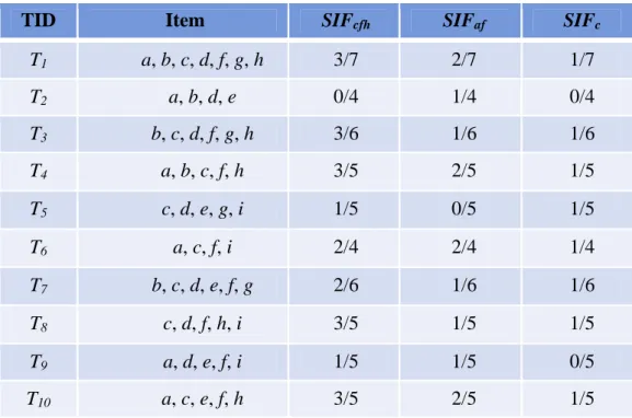
(30) Table 4-1: A database example with 10 transactions TID Item. T1. a, b, c, d, f, g, h. T2. a, b, d, e. T3. b, c, d, f, g, h. T4. a, b, c, f, h. T5. c, d, e, g, i. T6. a, c, f, i. T7. b, c, d, e, f, g. T8. c, d, f, h, i. T9. a, d, e, f, i. T10. a, c, e, f, h. Assume the set of user-specific sensitive itemsets S is {cfh, af, c}. Also assume the user-specific minimum support threshold is set at 40%, which indicates that the minimum count is 0.4*10, which is 4. The proposed approach proceeds as follows to hide the sensitive Itemsets for avoiding being mined from the database.. STEP 1: The transactions with sensitive itemsets in the database are found and kept. In this. example, all the 10 transactions contain at least one sensitive itemset. All of them are then kept for later processing.. STEP 2: The sensitive items frequency (SIF) value of each sensitive itemset in each. transaction is calculated. Take the first transaction as an example to illustrate the step. The first transaction includes the following seven items: {a, b, c, d, f, g, h}. The given sensitive itemsets. 19.

(31) include {cfh, af, c}. The appearing sensitive items in the first transaction for the sensitive itemset {cfh} are c, f, h, and the number is 3. Similarly, the numbers of the appearing sensitive items in the first transaction for the sensitive itemsets {af} and {c} are 2 and 1, respectively. Thus, the SIF values of each sensitive itemset in the first transaction are calculated as 3/7, 2/7 and 1/7, respectively. The SIF values of each sensitive itemset in the other transactions could be found in a similar way. The results are shown in Table 4-2.. Table 4-2: The SIF values of each sensitive itemset in each transaction TID Item SIFcfh SIFaf SIFc. T1. a, b, c, d, f, g, h. 3/7. 2/7. 1/7. T2. a, b, d, e. 0/4. 1/4. 0/4. T3. b, c, d, f, g, h. 3/6. 1/6. 1/6. T4. a, b, c, f, h. 3/5. 2/5. 1/5. T5. c, d, e, g, i. 1/5. 0/5. 1/5. T6. a, c, f, i. 2/4. 2/4. 1/4. T7. b, c, d, e, f, g. 2/6. 1/6. 1/6. T8. c, d, f, h, i. 3/5. 1/5. 1/5. T9. a, d, e, f, i. 1/5. 1/5. 0/5. T10. a, c, e, f, h. 3/5. 2/5. 1/5. STEP 3: The inverse database frequency (IDF) value of each sensitive itemset in each. transaction is calculated. In this step, the reduced count (RC) of each item for each sensitive itemset is first calculated and the maximum of the RC values of each item is found as the MRC value. Take item a as an example. The MRC value of item a is calculated as max{0, 5-0.4*10+1, 0}, which is max{0, 2, 0} and is equal to 2. The MRC values of the other items can be found in the same way. The results are shown in Table 4-3.. 20.

(32) Table 4-3: The MRC values of all the items RCcfh RCaf RCc. Item. MRC. a. -. 2. -. 2. b. -. -. -. 0. c. 2. -. 5. 5. d. -. -. -. 0. e. -. -. -. 0. f. 2. 2. -. 2. h. 2. -. -. 2. i. -. -. -. 0. The IDF value of each item is then calculated. Take item a as an example. The occurrence count of item a is 6 and the MRC value is 2. Its IDF value is then calculated as log(10/(6-2)), which is 0.398. The IDF values of all the items are shown in Table 4-4.. Table 4-4: The IDF value of each item Item Count MRC IDF. a. 6. 2. 0.398. b. 5. 0. 0.301. c. 8. 5. 0.523. d. 7. 0. 0.155. e. 5. 0. 0.301. f. 8. 2. 0.222. h. 5. 2. 0.523. i. 4. 0. 0.398. 21.

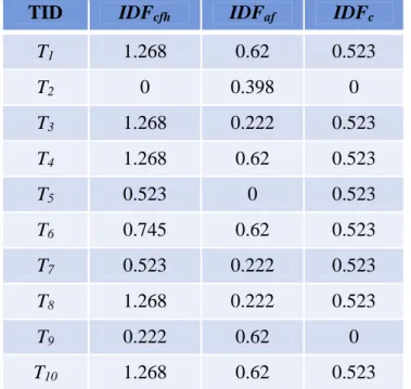
(33) The IDF value of each sensitive itemset in each transaction is then calculated. Take the first transaction for the first sensitive itemset {cfh} as an example to illustrate the process. The IDF value of {cfh} in the first transaction is the sum of the IDF values of the three items c, f and h, which is 0.523 + 0.222 + 0.523 and is equal to 1.268. All the results after this step are shown in Table 4-5.. Table 4-5: The IDF value of each sensitive itemset in each transaction TID IDFcfh IDFaf IDFc. T1. 1.268. 0.62. 0.523. T2. 0. 0.398. 0. T3. 1.268. 0.222. 0.523. T4. 1.268. 0.62. 0.523. T5. 0.523. 0. 0.523. T6. 0.745. 0.62. 0.523. T7. 0.523. 0.222. 0.523. T8. 1.268. 0.222. 0.523. T9. 0.222. 0.62. 0. T10. 1.268. 0.62. 0.523. The SIF-IDF value of an sensitive itemset in each transaction is then calculated as the SIF value of the sensitive itemset multiplied by its IDF value in the transaction. Take the first transaction as an example to illustrate the process. The SIF value of the sensitive itemset {cfh} in the first transaction is 3/7 as shown in Table 4-2, and its IDF value is 1.268 as shown in Table 4-5. The SIF-IDF value of {cfh} is then calculated as 3/7*1.268, which is 0.5434. The other SIF-IDF values for the two sensitive itemsets {af} and {c} are calculated as 0.1771 and 0.0747, respectively. That is, the SIF-IDF value of the first transaction is summed as 0.5434 + 0.1771 +. 22.

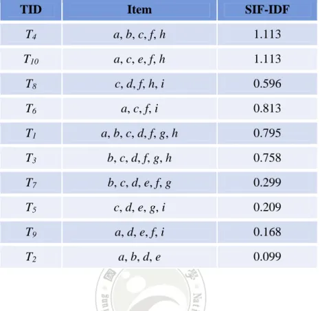
(34) 0.0747, which is 0.795. The other transactions are processed in the same way. After that, the results are shown in Table 4-6.. TID. Table 4-6: The SIF-IDF values for all the transactions IDF1 SIF2 IDF2 SIF3 IDF3 SIF1. SIF-IDF. T1. 3/7. 1.268. 2/7. 0.62. 1/7. 0.523. 0.795. T2. 0/4. 0. 1/4. 0.398. 0/4. 0. 0.099. T3. 3/6. 1.268. 1/6. 0.222. 1/6. 0.523. 0.758. T4. 3/5. 1.268. 2/5. 0.62. 1/5. 0.523. 1.113. T5. 1/5. 0.523. 0/5. 0. 1/5. 0.523. 0.209. T6. 2/4. 0.745. 2/4. 0.62. 1/4. 0.523. 0.813. T7. 2/6. 0.523. 1/6. 0.222. 1/6. 0.523. 0.299. T8. 3/5. 1.268. 1/5. 0.222. 1/5. 0.523. 0.901. T9. 1/5. 0.222. 1/5. 0.62. 0/5. 0. 0.168. T10. 3/5. 1.268. 2/5. 0.62. 1/5. 0.523. 1.113. STEP 4: The transactions in Table 4-6 are sorted in the descending order of their SIF-IDF. values. The results are then shown in Table 4-7.. 23.

(35) Table 4-7: The sorted transactions according to the SIF-IDF values TID Item SIF-IDF. T4. a, b, c, f, h. 1.113. T10. a, c, e, f, h. 1.113. T8. c, d, f, h, i. 0.596. T6. a, c, f, i. 0.813. T1. a, b, c, d, f, g, h. 0.795. T3. b, c, d, f, g, h. 0.758. T7. b, c, d, e, f, g. 0.299. T5. c, d, e, g, i. 0.209. T9. a, d, e, f, i. 0.168. T2. a, b, d, e. 0.099. STEP 5: The transactions are processed in the above descending order to prune appropriate. items. In this example, the set of sensitive itemsets is {cfh, af, c}. The occurrence frequencies of the items within the sensitive itemsets are {a:1, c:2, f:2, h:1}. The items are then sorted in the descending order of their frequencies as {c:2, f:2, a:1, h:1}, which will be used as the deletion sequence. From Table 4-7, transaction 4 has the best SIF-IDF value among all the ten. It is thus selected to be processed. The item c in transaction 4 is then first selected to be deleted.. STEP 6: After item c is deleted from the fourth transaction, the new occurrence. frequencies of the sensitive Itemsets in the transactions are updated. The sensitive itemsets with their occurrence frequencies are then updated from {cfh:5, af:5, c:8} to {cfh:4, af:5, c:7}.. 24.

(36) STEP 7: STEPs 2 to 6 are then repeated until the supports of all the sensitive itemsets are. below the minimum count. The results of the final sanitized database in the example are shown in Table 4-8.. Table 4-8: The result of the final sanitized database in the example TID Item. T1. a, b, d, f, g, h. T2. a, b, d, e. T3. b, c, d, g, h. T4. a, b, h. T5. c, d, e, g, i. T6. a, f, i. T7. b, c, d, e, f, g. T8. d, f, h, i. T9. a, d, e, f, i. T10. a, e, h. 25.

(37) Chapter 5 A Greedy Approach Based on Lattices. The Apriori mining algorithm [5] uses the downward closure property to efficiently generate and test itemsets level-by-level. The process can be represented by a lattice structure as shown in Figure 5-1.. Figure 5-1: A lattice structure with five items. In this chapter, a lattice-like algorithm for privacy-preserving data mining (PPDM) is then proposed for efficiently hiding the sensitive itemsets. The measure Extra Count (EC) of a sensitive itemset is first defined below:. 26.

(38) EC j = f j − s * n + 1, where f j is the occurrence frequency of a sensitive itemset sij, s is the user-specific support threshold, and n is the number of transactions in database, 1 ≤ j ≤ m . In the lattice-like approach, it treats all the sensitive itemset as the initial sets in the lattice structure. For example in Figure 5-2, the three itemsets S1, S2, and S3 are sensitive, and put in the first level (as the initial sets) of the lattice. All the combinations from the initial sets are then level-wisely created by the union operation on the items contained. The corresponding transactions in each set of the lattice structure can thus be found through the intersection operation of the combined sets. For the above example, the lattice structure is built as shown in Figure 5-2.. Figure 5-2: The lattice structure built from the three sensitive itemsets. For support-based approaches of PPDM, the supports of all the sensitive itemsets must be under the user-specific support threshold. In the proposed lattice-like approach, the item removal. 27.

(39) process is performed from the higher levels to the lower ones. For example in Figure 5-2, the set at level 3 is first processed. It has three sensitive itemsets and the one with the minimal EC value is found. If the transaction number in the node is larger than or equal to EC, then totally EC transactions in the processed set in the node are randomly selected and the items contained in the selected sensitive itemset are deleted from them. Otherwise, all the transactions in the node are used to delete the items in the selected itemset. After that, the EC values of the remaining sensitive itemsets are updated for the next processing. This procedure is repeated until the EC values of all the sensitive values become 0. The flowchart of the proposed lattice-like approach is shown in Figure 5-3. The proposed algorithm and an example are described in the next sections, respectively.. 28.

(40) Calculate EC for each sensitive itemset. Create the lattice structure. Process the nodes bottom-up in the lattice structure. Find the sensitive itemset with the minimal EC in the corresponding node of the current level. Select the transactions in the node. Delete items from the selected transactions. Update EC values. N. Satisfy termination condition?. Y Output the sanitized database. Figure 5-3: The flowchart of the proposed lattice-like approach. The details of the proposed algorithm are described below.. 29.

(41) 5.1. The Proposed Lattice-Like Algorithm. INPUT: A transaction dataset D = {T1, T2, …, Ti, …, Tn}, a set of p items I = {i1, i2, …, ik, …,. ip}, a user-specific minimum support threshold s, and a set of m user-defined sensitive itemsets S_Items = {si1, si2, …, sij, …, sim}. OUTPUT: A sanitized database. STEP 1: Calculate the Extra Count (ECj) value of each sensitive itemset sij as:. EC j = f j − s * n + 1, where f j is the occurrence frequency of the sensitive itemset sij, and n is the number of transactions in the database, 1 ≤ j ≤ m . STEP 2: Create the lattice structure from the lowest level to the highest one by the following. substeps. Substep 2-1: Create a node for each itemset in the first level of the lattice and attach. the transactions including the itemset to the corresponding node. Substep 2-2: Initially set k = 1, where k is the level to be processed. Substep 2-3: Generate the nodes in the (k+1)-th level from the nodes in the k-th level. through the combination process. Substep 2-4: Set the items of a node in the (k+1)-th level as the union of the items in. its associated nodes in the k-th level. Substep 2-5: Set the transactions of a node in the (k+1)-th level as the intersection of. the transactions in its associated nodes in the k-th level. Substep 2-6: Repeat Substeps 2-3 to 2-5 until all the levels are processed.. 30.

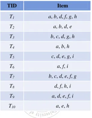
(42) STEP 3: Process the nodes bottom-up (from the highest level to the lowest level) in the lattice. structure by the following substeps. Substep 3-1: Find the nodes to be processed which corresponding the minimal EC. value is larger than 0. Substep 3-2: Find the sensitive itemset with the minimal EC value. Substep 3-3: If the transaction number in the corresponding node is larger than or. equal to EC, then totally EC transactions in the node are randomly selected. Substep 3-4: If the transaction number in the node is less than EC, then all of. transactions in the node are selected. Substep 3-5: Delete the items of the processed sensitive itemset from the selected. transactions. Substep 3-6: Update the EC values of all the sensitive itemsets. Substep 3-7: Repeat STEP 3 until the EC values of all the sensitive itmesets become. 0.. 5.2. An Example. In this section, an example is given to demonstrate the proposed lattice-like approach for privacy preserving data mining (PPDM). Assume the database shown in Table 5-1 is used for PPDM. It consists of 10 transactions and 9 items, denoted a to i. A set called S_Items contains the user-specific sensitive Itemsets. In this example, assume S_Items = {cfh, af, c}. The user-specific. 31.

(43) minimum support threshold is set at 40%, which indicates the minimum count is 0.4*10, which is 4.. Table 5-1: An example database with 10 transactions TID. Item. 1. a, b, c, d, f, g, h. 2. a, b, d, e. 3. b, c, d, f, g, h. 4. a, b, c, f, h. 5. c, d, e, g, i. 6. a, c, f, i. 7. b, c, d, e, f, g. 8. c, d, f, h, i. 9. a, d, e, f, i. 10. a, c, e, f, h. STEP 1: The Extra-Count (EC) value of each sensitive itmeset is first calculated. In this. example, the occurrence frequencies of the three sensitive itemsets {cfh, af, c} are 5, 5, and 8, respectively. That is, the EC values of the three sensitive itemsets {cfh, af, c} are computed as 5-0.4*10+1, 5-0.4*10+1, 8*0.4*10+1, which are 2, 2, and 5, respectively. STEP 2: Create the lattice structure: Substep 2-1: According to user-specific sensitive itemsets {cfh, af, c}. Create three. nodes S1, S2 and S3 are then assigned to the sensitive itemsets {cfh}, {af}, and {c}, respectively. The corresponding transactions of node S1 are {T1, T3, T4, T8, T10}, which contains the sensitive itemset {cfh}. The node for. 32.

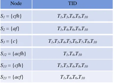
(44) S2 and S3 are also processed in the same way. The results are then shown in Table 5-2.. Table 5-2: The corresponding transactions of three sets. Node. TID. S1 = {cfh}. T1,T3,T4,T8,T10. S2 = {af}. T1,T4,T6,T9,T10. S3 = {c}. T1,T3,T4,T5,T6,T7,T8,T10. Substep 2-2: The variable of k-level is initially set at 1. Substep 2-3: According to nodes {S1, S2, S3} in 1-th level. The combination procedure. for three nodes is to generate nodes of k+1 level. S1 and S2 combine to. S12, S2 and S3 combine to S23 and S1 and S3 combine to S13. Substep 2-4: Take node S12 as an example to illustrate the process. The itemset of. node S1 is {cfh} and the itemset of node S2 is {af}. The itemset of node. S12 is then composed as {cfh ∪ af} {= acfh}. The other nodes for S13 {= ach} and S23 {= acf} are processed in the same way in 2-level, respectively. Substep 2-5: The corresponding transactions for the generated nodes in Figure 5-4 are. thus found through intersection operation. Take node S12 as an example to illustrate the process. The corresponding transactions of node S1 and S2 are {T1, T3, T4, T8, T10} and {T1, T4, T6, T9, T10} shown in Table 5-2. The corresponding transactions of S12 are {T1, T3, T4, T8, T10 ∩ T1, T4, T6, T9,. 33.

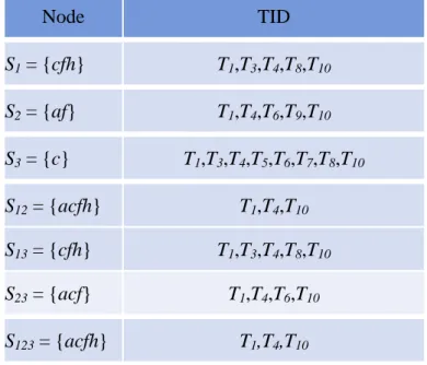
(45) T10} {= T1, T4, T10}. The corresponding transactions of the other generated nodes are processed in the same way and shown in Table 5-3.. Figure 5-4: The lattice structure after complete the combination procedure in 2-level. Table 5-3: The corresponding transactions of the nodes in 2-level. Node. TID. S1 = {cfh}. T1,T3,T4,T8,T10. S2 = {af}. T1,T4,T6,T9,T10. S3 = {c}. T1,T3,T4,T5,T6,T7,T8,T10. S12 = {acfh}. T1,T4,T10. S13 = {cfh}. T1,T3,T4,T8,T10. S23 = {acf}. T1,T4,T6,T10. Substep 2-6: Repeat Substeps 2-3 to 2-5 created the 3-level lattice structures. The. complete structures show as Figure 5-5 and the final corresponding transactions of each nodes show as Table 5-4.. 34.

(46) Figure 5-5: The lattice structure after complete the combination procedure. Table 5-4: The corresponding transactions of the all node in lattice structures. Node. TID. S1 = {cfh}. T1,T3,T4,T8,T10. S2 = {af}. T1,T4,T6,T9,T10. S3 = {c}. T1,T3,T4,T5,T6,T7,T8,T10. S12 = {acfh}. T1,T4,T10. S13 = {cfh}. T1,T3,T4,T8,T10. S23 = {acf}. T1,T4,T6,T10. S123 = {acfh}. T1,T4,T10. STEP 3: The lattice structures in Figure 5-4 are then sequentially processed bottom-up from the. highest level (3-level) to the lowest level (1-level).. 35.

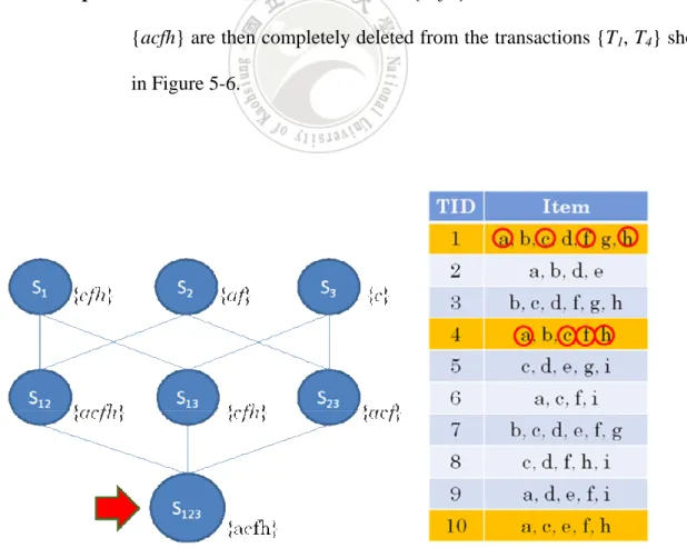
(47) Substep 3-1: In this example, the EC values for three nodes S1 = {cfh}, S2 = {af} and. S3 = {c} are {2, 2, 5}. The minimal EC value of node S123 is min{2, 2, 5} {= 2} larger than 0. That is, the node S123 wants to process. Substep 3-2: The sensitive itemset of node S123 is {acfh}. Substep 3-3: For node S123 in Table 5-4, it contains three transactions {T1, T4, T10}.. From the results in Substep 3-1, the minimal EC value of set S123 is 2. Because the transaction number in S123 is large than EC value, we randomly select two transactions from the corresponding transactions {T1,. T4, T10} of S123. In this example, suppose we select the transactions {T1, T4} as the processed transactions for later process. Substep 3-5: In the node S123, it contains items {acfh} shown in Table 5-4. The items. {acfh} are then completely deleted from the transactions {T1, T4} shown in Figure 5-6.. Figure 5-6: The deletion process of items {acfh} in S123. 36.

(48) Substep 3-6:The EC values of three nodes S1, S2 and S3 are then updated. Since the. items {acfh} are deleted from two transactions, the EC values for three nodes S1, S2 and S3 are then updated as {2-2, 2-2, 5-2} {= 0, 0, 3}. STEP 3: The steps 3 is repeated until the EC values of three sets become 0. In this example, the. node in 2-level are then processed. Substep 3-1: Take the set S12 as an example to illustrate the process, which is shown in. Figure 5-7.. Figure 5-7: The deletion process of set S12. The minimal EC value of set S12 is min{0, 0} {= 0}. That is, it is unnecessary to process any steps in this set. The other sets S13 and S23 are processed in the same way. In this example, the minimal EC values for. 37.

(49) sets S13 and S23 are 0. That is, it is unnecessary to process any steps for sets S13 and S23. STEP 3: The procedure moves to 1-level to process it. Substep 3-1: The procedure moves to 1-level to process it. In 1-level, since the EC. values for S1 and S2 are 0. That is, it is unnecessary to process any steps for nodes S1 and S2. Substep 3-2: For the node S3, the sensitive itemsets is {c}. Substep 3-3:For the node S3, the minimal EC value is calculated as min{3} {= 3}.. The corresponding transactions of S3 are {T1, T3, T4, T5, T6, T7, T8, T10} shown in Table 5-4. That is, we randomly select three transactions from the corresponding transactions {T1, T3, T4, T5, T6, T7, T8, T10} of S3. In this example, suppose we select the transactions {T3, T5, T6} as the processed transactions for later process. Substep 3-5: Delete item {c} from the transactions {T3, T5, T6}, shown in Figure 5-8. Substep 3-6: Since the item {c} is deleted from three transactions, the EC values for. S3 is then updated as {3 - 3} {= 0}. That is, all EC values for three sensitive itemsets become 0, the procedure of lattice-like approach is thus terminated. The output results of sanitized database are then shown in Table 5-5.. 38.

(50) Figure 5-8: The deletion process of item {c} in set of S3. Table 5-5: The output result of sanitized database with lattice-like approach TID. Item. 1. b, d, g. 2. a, b, d, e. 3. b, d, f, g, h. 4. b. 5. d, e, g, i. 6. a, f, i. 7. b, c, d, e, f, g. 8. c, d, f, h, i. 9. a, d, e, f, i. 10. a, c, e, f, h. 39.

(51) Chapter 6 A GA-Based Approach for PPDM. This section introduces is an evolutionary privacy-preserving data mining method, which finds appropriate transactions to be hidden from a database. The proposed approach designs a flexible evaluation function with three factors, and different weights may be assigned to them depending on users’ preference. Besides, the concept of pre-large itemsets is used to reduce the cost of rescanning a database, thus speeding up the evaluation process of chromosomes. The details of the algorithm are stated below. First, the chromosome representation is described.. 6.1. Chromosome Representation In GAs, a chromosome corresponds to a possible feasible solution. The goal here is to hide. at most m appropriate transactions from a database such that the fitness value can be optimal. Thus, a chromosome with m genes is used, with each gene representing a possible transaction to be hidden. A positive integer for a transaction ID or the number zero is kept in a gene. If the value of a gene is zero, it represents that there is no transaction needing to be deleted. An example for the chromosome representation used in this thesis is shown in Figure 6-1. It represents that the four transactions T2, T3, T4, and T5 will be deleted from the original database for privacy preserving.. g1. g2. g3. g4. 2. 3. 4. 5. Figure 6-1: An example for a chromosome 40.

(52) 6.2. Fitness Function GAs need to set fitness functions to evaluate the goodness of chromosomes. Different. application domains may need different fitness functions. In PPDM, the purpose is to hide sensitive items but reduce side effects. The relationship of itemsets before and after the PPDM process can be depicted in Figure 6-2, where L represents the large itemsets of D, S represents the sensitive itemsets defined by users that are large, ~S represents the non-sensitive itemsets that are large, and L’ is the large itemsets after some records are deleted.. Figure 6-2: The relationship of itemsets before and after the PPDM process. 41.

(53) Let α be the number of sensitive itemsets that fail to be hidden. That is, it is the number of sensitive itemsets that still appear after the sanitization process. Ideally, the value should be zero after PPDM. This set of sensitive itemsets can be depicted in Figure 6-3, in which the α part is the interaction of S and L’.. α. Figure 6-3: The set of sensitive itemsets that fail to be hidden. Another evaluation criterion is the number of missing itemsets, which is denoted as β . A missing itemset is a non-sensitive large itemset in the original database, but is not mined out from the sanitized database. This side effect is shown in Figure 6-4, in which the β part is the difference of ~S and L’.. 42.

(54) β. Figure 6-4: The set of missing itemsets. The last evaluation criterion is the number of artificial itemsets, which is denoted γ . It represents the set of large itemsets appearing in the sanitized database but not belonging to the large itemset in the original database. This side effect is shown in Figure 6-5, in which the γ part is the the difference of L’ and L.. 43.

(55) L. ~S. S. L. γ. Figure 6-5: The set of artificial itemsets. From Figures 6-3 to 6-5, it is known that α = S ∩ L' , β = ~ S − L' = ( L − S ) − L' , and γ = L' − L . The fitness function used in the chapter may be defined as follows:. fitness = ω1 × α + ω2 × β + ω3 × γ ,. (6). where ω1 , ω2 and ω3 are the weighting parameters. Besides, the fitness values can be easily evaluated without database rescan by pre-large itemsets. It is discussed as follows.. 44.

(56) The traditional methods for evaluating the fitness value need to rescan the database to calculate the three numbers, thus spending a lot of computation cost. The problem can be eased by pre-large itemsets [12]. They act like buffers and are used to reduce the movement of itemsets directly from large to small and vice-versa when transactions are deleted. In the GA-based approach, the pre-large concept is used in evaluating the fitness values for saving the database rescan time. When few records are deleted from the database, the results can be easily derived without re-scanning the whole database through the help of stored pre-large itemsets. The concept of pre-large itemsets is used here to reduce the cost of rescanning a database and to speed up the evaluation process of chromosomes.. 6.3. Genetic Operators Genetic operators are very important to the success of specific GA applications. The. operators used in the thesis are described as follows.. 6.3.1 Crossover A crossover operator considers two chromosomes to generate new offspring. It is the main genetic operator in GAs. There have been several crossover operators developed, such as the single-point crossover, the two-point crossover, the uniform crossover and the arithmetic crossover, among others. The single-point crossover is used here to generate new offspring shown in Figure 6-6.. 45.

(57) Figure 6-6: The crossover operator. 6.3.2 Mutation The purpose of mutation is to diversify the search direction and prevent converging to local optima. Mutation usually produces some random changes in chromosomes, but there is no guarantee that mutation will produce desirable features in the new chromosomes. In the proposed approach, the adopted mutation operator will change the integer value in a selected gene to another integer. An example is shown in Figure 6-7.. Figure 6-7: The mutation operation 46.

(58) 6.3.3 Selection The selection operation chooses some offspring for survival according to predefined rules. This keeps the population size under good control. There has been several selection methods proposed, such as Elitism, Rank, Tournament, and Roulette-Wheel. In this paper, we propose a hybrid selection method, which combines the Elitism approach and the Rank approach. First, the chromosomes in the population are sorted by their fitness values. The top b (usually n/2) chromosomes in the list are then selected to the next population, where n is the population size. Next, p (= n–b) chromosomes are randomly selected from the original database to the next population. The selection mechanism may be illustrated in Figure 6-8.. Figure 6-8: The selection mechanism. 47.

(59) The flowchart of the proposed GA-based approach is shown in Figure 6-9. The algorithm is described in the next section.. Figure 6-9: The flowchart of the GA-based approach for PPDM. 6.4. The Proposed GA-based Algorithm for PPDM. The proposed GA-based algorithm for PPDM is stated as follows.. 48.

(60) The algorithm: INPUT: A transaction dataset D, a minimum support threshold s, a set of sensitive itemsets. defined by users, and the maximum number m of transactions to be hidden, and a population size n. OUTPUT: An appropriate set of transactions to be hidden. STEP 1: Derive the lower support threshold Sl as:. ⎛ m ⎞ sl = su × ⎜ 1 − ⎟. ⎝ | D|⎠ STEP 2: Scan the database to find the large and the pre-large itemsets. STEP 3: Randomly generate a population of n individuals with m genes, with each gene being. the ID number of the transaction to be hidden. STEP 4: Calculate the fitness value of each chromosome Ci in the population as:. fitness(i ) = ω1 × α i + ω2 × βi + ω3 × γ i , where ω1 , ω2 and ω3 are weighting parameters, α is the number of sensitive itemsets that fail to be hidden, β is the number of missing itemsets, and γ is the number of artificial itemsets. STEP 5: Execute the crossover operations on the population. STEP 6: Execute the mutation operations on the population. STEP 7: Choose the top b chromosomes from the population and randomly select p. chromosomes from the original database to generate the n chromosomes in the next population. STEP 8: If the termination criterion is not satisfied, go to Step 4; otherwise, do the next step. 49.

(61) STEP 9: Output the hidden transaction numbers in the best chromosome to users.. 6.5. An Example. In this section, an example is given to demonstrate the proposed GA-based algorithm for privacy preserving data mining. Assume the original database includes 10 transactions, as shown in Table 6-1. Each transaction consists of its transaction identification (TID) and items. Also assume that the set of sensitive itemsets is defined as {be, bce} and the minimum support threshold rate s is 40%. Thus, the upper threshold count Su is set as 10*40%, which is 4. Let the allowed maximum number m of deleted records be 4. The proposed algorithm processes the data as follows.. Table 6-1: The set of the original database in the example TID. Item. 1. a, b, c. 2. b, c, e. 3. a, b, c, e. 4. a, b, e. 5. a, b, e. 6. a, c, d. 7. b, c, d, e. 8. b, c, e. 9. c. 10. a, b. 50.

(62) STEP 1: The lower threshold (Sl) can be calculated as 0.24 according to the formula. ⎛ m ⎞ sl = su × ⎜ 1 − ⎟ . The lower threshold count is the floor of 4*(1-4/10), which is 2. ⎝ | D|⎠ STEP 2: After the lower threshold is obtained, the original database is then processed to get the. large and the pre-large itemsets. The large itemsets with different item numbers are shown in Tables 6-2, 6-3 and 6-4, respectively. The pre-large Itemsets with different numbers are shown in Tables 6-5, 6-6 and 6-7.. Table 6-2: Large 1-itemsets Item. Count. a. 6. b. 8. c. 7. e. 6. Table 6-3: Large 2-itemsets Item. Count. ab. 5. bc. 5. be. 6. ce. 4. Table 6-4: Large 3-itemsets Item. Count. bce. 4. 51.

(63) Table 6-5: Pre-Large 1-itemsets Item. Count. d. 2. Table 6-6: Pre-Large 2-itemsets Item. Count. ac. 3. ae. 3. cd. 2. Table 6-7: Pre-Large 3-itemsets Item. Count. abc. 2. abe. 3. STEP 3: A population of n individuals with m genes is randomly generated. In this example, at. most four transactions are to be deleted, such that each chromosome is composed of four genes. For example, assume the four transactions T2, T3, T4, and T5 are randomly selected to form an initial chromosome. Its chromosome representation is thus (2, 3, 4, 5). STEP 4: The fitness value of each chromosome in the population is evaluated. Assume the. chromosome (2, 3, 4, 5) exists in the current population. For evaluating the chromosome, the resulting large itemsets after the four transactions represented by the chromosome are deleted need to be obtained. They may easily derived without database rescan with the aid of the pre-large itemsets. First, the database size d is updated from 10 to 6 when the four transactions are deleted from the database. Since the minimum support threshold is 40%, the upper count threshold is thus updated to. 52.

(64) the ceiling of 6*40%, which is 3. The original large itemsets and pre-large itemsets are then updated according to the items in the deleted transactions, with the results shown in Figure 6-7. The final large itemsets are thus {a}, {b}, {c} and {bc}.. Figure 6-10: The large itemsets after the four transactions are deleted. After the large Itemsets are obtained, the number (α) of sensitive itemsets that fail to be hidden, the number (β) of missing itemsets, and the number (γ) of artificial Itemsets can be easily obtained. In the above example, the set of sensitive itemsets that fail to be hidden is {be, bce} ∩ {a, b, c, bc}, which is Ø. The value of α is thus 0. The set of missing itemsets is ({a, b, c, e, ab, bc, be, ce, bce} - {be, bce}) – {a, b, c,. bc}, which is {e, ab, ce}. The value of β is thus 3. The set of artificial itemsets is Ø. The value of γ is thus 0. Let the three weight parameters are set as 0.5, 0.25, and 0.25, respectively. The fitness value of the chromosome is then calculated as follows:. 53.

(65) fitness = 0.5 × 0 + 0.25 × 3 + 0.25 × 0 = 0.75 . STEP 5: The crossover operation is executed on the population. An example has been. previously shown in Figure 6-6. STEP 6: The mutation operation is executed on the population. An example has been. previously shown in Figure 6-7. STEP 7: In the selection step, we set b as n/2. Thus, the top b chromosomes from the current. population and the randomly chosen p (= n-b) chromosomes from the original database are gathered to form the new population by the selection scheme. STEP 8: If the results of the new population do not satisfy the termination condition, then Steps. 4 to 7 are repeated; otherwise, the algorithm is stopped. In the example, two criteria are uses as the termination condition. The first one is the fitness function value of the best chromosome is 0, and the other one is a predefined number of generations is achieved.. 54.