國 立 交 通 大 學
電 控 工 程 研 究 所
碩 士 論 文
應用人體動作辨識系統於吃藥辨識及日常生活
活動
Applying Human Activity Recognition System to Medicine
Taking and Activities of Daily Living
研 究 生 : 蔡 宗 憲
指 導 教 授: 張 志 永
應用人體動作辨識系統於吃藥辨識及日常生活
活動
Applying Human Activity Recognition System to Medicine
Taking and Activities of Daily Living
學 生 : 蔡宗憲 Student : Tzung-Shian Tsai
指導教授 : 張志永 Advisor : Jyh-Yeong Chang
國立交通大學
電控工程研究所
碩士論文
A Thesis
Submitted to Department of Electrical Engineering
College of Electrical Engineering
National Chiao-Tung University
in Partial Fulfillment of the Requirements
for the Degree of Master in
Electrical and Control Engineering
July 2011
Hsinchu, Taiwan, Republic of China
中 華 民 國 一百 年 七 月
應用人體動作辨識系統於吃藥辨識及日常生活活動
學生:蔡宗憲 指導教授: 張志永博士
國立交通大學電機與控制工程研究所
摘要
人體動作辨識系統在電腦視覺領域一直是很熱門的研究與應用目標。在居家 監控系統中最常見的方式是,使用固定式的攝影機,對室內的人物進行追蹤與動 作辨識。為了達到即時監控之目標,處理的演算法必須快速,而且又必須能夠有 效的分析影像。 在本論文中,動作辨識的目標是人體,為了更正確的擷取出人體部份,我們 同時使用灰階域與 HSV 色彩空間,建立兩個背景模型,提升消除影像中陰影部 分之效果,使得前後景之分離結果能夠更完整。我們以 5:1 降低取樣頻率,取 得即時影像,擷取出的前景部份,經過特徵空間轉換與標準空間轉換後,累積三 張上述降頻取樣動作影像後,藉由預先學習而建立之模糊法則與時序動作姿態比 對,完成人體動作之辨識。 此外,當某人要進行吃藥動作時,我們使用在 HSV 空間中建立好的藥包顏 色色彩模型(僅考慮色調)去辨識藥包的顏色。因此,藉由結合藥包顏色色彩模 型和人體動作辨識系統,我們就可以得知某人正在吃藥以及他的藥包顏色。最 後,我們利用人體動作辨識系統去記錄學生的日常生活。Applying Human Activity Recognition System to
Medicine Taking and Activities of Daily Living
STUDENT: Tzung-Shian Tsai ADVISOR: Dr. Jyh-Yeong ChangInstitute of Electrical and Control Engineering National Chiao-Tung University
ABSTRACT
Human activity recognition system is now a very popular subject for research and application. Using a fixed camera to track a person and recognize his (her) activity is widely seen in home surveillance. For real-time surveillance, the embedded algorithms must be efficient and fast to meet the real-time constraint.
In the thesis, a new person tracking and continuous activity recognition is proposed. We build two background models, in grayscale and HSV color space as well to extract the human correctly, and we could also reduce the shadowing effect well. For better efficiency and separability, the binary image is firstly transformed to a new space by eigenspace and then canonical space transformation, and the recognition is finally done in canonical space. A three image frame sequence, 5:1 down sampling from the video, is converted to a posture sequence by template matching. The posture sequence is classified to an action by fuzzy rules inference. Fuzzy rule approach can not only combine temporal sequence information for recognition but also be tolerant to variation of action done by different people and time.
Moreover, we make use of the hue component to recognize the medical pouch’s color when one is taking medicine. By combining with the hue-based pouch’s color model and human activity recognition system, we can know someone is taking medicine and its medical pouch’s color as well. Finally, we also employ the activity
ACKNOWLEDGEMENTS
I would like to express my sincere gratitude to my advisor, Dr. Jyh-Yeong Chang for valuable suggestions, guidance, support and inspiration he provided. Without his advice, it is impossible to complete this research. Thanks are also given to all the people who assisted me in completing this research.
Finally, I would like to express my deepest gratitude to my family for their concern, supports and encouragements.
Contents
摘要 ...………..………...i
ABSTRACT ……….……….…...ii
ACKNOWLEDGEMENTS ……….………..iv
Contents ………...v
List of Figures ………..viii
List of Tables ……….……….xi
Chapter 1 Introduction ………1
1.1 Motivation of this research ………1
1.2 Foreground subject extraction ………4
1.3 Eigenspace and Canonical Space Transformation ………….……...………4
1.4 Image Frame Classification and Activity Recognition ………….…………5
1.5 Thesis Outline ………7
Chapter 2 Basic Concept ………8
2.1 Fundamentals of Eigenspace and Canonical Space Transform ………8
2.1.1 Eigenspace Transformation (EST) ..………10
2.2 The HSV color space ..………14
Chapter 3 Taking Medicine Recognition System ………17
3.1 Skin Color Detection ………18
3.2 Medical Pouch Color Recognition ………22
3.3 Human Activity Recognition System ...………..24
3.3.1 Object Extraction ……..………24
A. Background Model ………….…….……...………24
B. Extraction of Foreground Object ………26
C. Shadow Suppression ………..28
D. Object Segmentation ………..30
E. Foreground Image Compensation ...………31
3.3.2 Background Update ...…………..………32
3.3.3 Activity Template Selection ……….32
3.3.4 Construction of Fuzzy Rules for Video Stream ………35
3.3.5 Classification algorithm ………...………39
Chapter 4 Experimental Results ...40
4.1.1 Skin Color Detection and Medical Pouch Color Detection ………41
4.1.2 Medical Pouch Color Detection ………...44
4.2 Background Model and Object Extraction ………..………48
4.3 Fuzzy Rule Construction for Action Recognition ………51
4.4 The Recognition Rate of Activities ……….55
4.5 The Activities of Daily Living ………57
Chapter 5 Conclusion ………64
List of Figures
Fig. 1.1 The block diagram of human activity recognition system. …….……….3
Fig. 2.1 The HSV Cone. ……….………...……..14 Fig. 3.1 The block diagram of taking medicine recognition system. ……..…………17 Fig. 3.2 Scene 1, normal view on medical pouch table. ……..………18
Fig. 3.3 Scene 2, zoom-in of Scene 1 and being used to recognize medical pouch’s
color. ………..………18
Fig. 3.4 Original image Ioriginal in s2. …….……….………20 Fig. 3.5 The binary image Iskin, in which white. ….………..…… 20 Fig. 3.6 Histogram of binary image Iskin projection in the X and Y directions. ...…21 Fig. 3.7 A rectangular region is detected to confine the subject’s hands. ………22
Fig. 3.8 The structure of the medical pouch color recognition in the i -th image. …23
Fig. 3.9The framework we apply to foreground subject extraction. ………... 26
Fig. 3.10Histogram of binary image projection in X and Y direction. …....……….. 31
Fig. 3.11 The binary image of extracted foreground region. ...…….………. 31
Fig. 3.12 One image frame is selected as template with an interval. .…...……….. 33
Fig. 3.13 Common states of two different activities. ………...35
Fig. 4.1 Scene 1, normal view on medical pouch table. .………40 Fig. 4.2 Scene 2, zoom-in of Scene 1 and being used to recognize medical pouch’s color. ………..40
image frame, (b) kskin=40, (c) kskin=45, (d) kskin=50, (e) kskin=55, (f) kskin=60. ...42
Fig. 4.4 An example of hand region extraction. (a) An image frame, (b) binary image after skin color analysis, (c) projection of (b) onto X direction, (d) projection of (b) onto Y direction, (e) hand region extracted. ...43
Fig. 4.5 Some pouch’s color images in analytic phase. (a) red data, (b) green data, (c)yellow data. ……….44
Fig. 4.6 Histogram plot of hue component in the red data. …….………45
Fig. 4.7 Histogram plot of hue component in the green data. …….………45
Fig. 4.8 Histogram plot of hue component in the yellow data. …...………46
Fig. 4.9 An example of foreground extraction (a) An image frame, (b) after using background models, (c) after using shadow filter, (d) after using closing filter, (e) after using opening filter. ……….………..49
Fig. 4.10 An example of foreground region extraction. (a) An image frame, (b) binary image after background analysis, (c) projection of (b) onto X direction, (d) projection of (b) onto Y direction, (e) foreground region extracted. ………..………..50
Fig. 4.11 Some “essential templates of posture” of model 1. ...………..52
Fig. 4.12 Corresponding “essential templates of posture,” Fig. 4.11, of model 2. ….53 Fig. 4.13 The activities of daily living in (a) the morning of 6/20, (b) the afternoon of 6/20. ……….58
Fig. 4.14 The activities of daily living in (a) the morning of 6/21, (b) the afternoon of 6/21. ……….59
Fig. 4.15 The activities of daily living in (a) the morning of 6/23, (b) the afternoon of 6/23. ……….60
Fig. 4.16 The activities of daily living in (a) the morning of 6/24, (b) the afternoon of 6/24. ……….61
Fig. 4.17 The activities of daily living in (a) the morning of 6/29, (b) the afternoon of 6/29. ……….62
List of Tables
TABLE I COLOR RECOGNITION RESULT OF THE RECOGNITION RATES …….………47
TABLE II The Recognition Rate of Person 2 with Different Starting Frame ………56
TABLE III THE RECOGNITION RATES OF FOUR FOLDS CROSS VALIDATION OF EACH
ACTIVITY .………57
Chapter 1 Introduction
1.1 Motivation of this research
Human activity analysis is an open problem that has been studied intensely within the areas of video surveillance, homeland security, and more recently, eldercare. In the video surveillance, human activity recognition from video streams has many applications such as home care system, human-machine interface, automatic surveillance, and smart home applications. For example, an automatic system will trigger an alarm condition when the automated surveillance system detects and recognizes suspicious human activities. Human activity recognition can also be used in extracting semantic descriptions from video clips to automate the process of video indexing. However, there is no rigid syntax and well-defined structure as that of the gesture and sign language which can be used for activity recognition. Therefore, this makes human activity recognition become a challenging task.
Several human activity recognition methods have been proposed in the past few years. Bobick and Davis [1], they recognized human activities by comparing motion-energy and motion-history of template images with temporal images. Carlsson and Sullivan [2], shape was represented by edge data obtained from canny edge detection. Cohen and Li [3] presented a view-independent 3-D shape description for classifying and identifying human activity using SVM. W4 [4] can detect people (single person or people in group) by adopting an adaptive background model and identify the activities by finding the body parts on the silhouette boundary. Luke and Keller et al. [5], they build a voxel person to model human activity and recognize these activities by fuzzy logic.
2
In our research, we design a robust method that uses temporal information, which is implicitly inherent in the human activity recognition. People have the same postures and posture sequences when they perform a specific action. Therefore, we use shape features to classify each image frame into postures we defined. Then, we use the frame sequences of key postures to recognize which activity one does. The objective of this thesis is to provide a system to auto-surveillance and to track people and identify their activities.
The human activity recognition system flowchart is illustrated in Fig. 1.1. Our system can be separated into three components. The first component is foreground subject extraction. The second component is the transformation of image data in a space smaller and easier for posture recognition. The third component is the posture classification of an image frame and activity recognition using frame sequences.
4
1.2 Foreground subject extraction
Background subtraction is widely used for detecting moving objects from image frames of static cameras. The rationale of this approach is to detect the moving objects by the difference between the current frame and a reference frame, often called the “background model.” A review is given in [6] where many different approaches were proposed in recent years. In our system, we build two background models; one is based on grayscale value and the other is based on HSV color space. Basically, the background image is a representation of the static scene. We prepare to update the background model until the subject enters the scene. After the subject leaves the scene, we also update the background mode.
After building a background model, we can extract foreground subject from video frames by subtracting each pixel value of background model from that current image frame. Then, the resulting image is converted to a binary image by setting a threshold. The binary image mainly contains foreground subject with only little noise. Therefore, we can set a threshold in the histogram of the binary image to extract a rectangle image, which is the most resemble shape of a person, of the target subjects. The rectangle image is resized to the standard level.
1.3 Eigenspace and Canonical Space Transformation
In most of video and image processing, the size of frame is usually very large and it usually exists some redundancy. The redundancy possesses little information of an image. Hence, some space transformations are introduced to reduce redundancy of an image by reducing the data size of the image. The first step of redundancy
reduction often transforms an image from spatiotemporal space to another data space. The transformation can use fewer dimensions to approximate the original image. There are many well-known transformation methods such as Fourier transformation, wavelet transformation, Principal Component Analysis and so on. Our transformation method combines eigenspace transformation and canonical space transformation which are described as follows.
Eigenspace transformation (EST), based on Principal Component Analysis, has been demonstrated to be a potent scheme used below: automatic face recognition proposed in [7], [8]; gait analysis proposed in [9]; and action recognition proposed in [10]. The subsequent transformation, Canonical space transformation (CST) based on Canonical Analysis, is used to reduce data dimensionality and to optimize the class separability and improve the classification performance. Unfortunately, CST approach needs high computation efforts when the image is large. Therefore, we combine EST and CST in order to improve the classification performance while reducing the dimension, and hence each image can be projected from a high-dimensional spatiotemporal space to a single point in a low-dimensional canonical space. In this new space the recognition of human activities becomes much simpler and easier.
1.4 Image Frame Classification and Activity Recognition
In this thesis each in a video segmentation, images are transformed into an image feature vector by extracting features from images. We extract image features by using eigenspace transformation and canonical space transformation. We group three contiguous 5:1 down-sampled images and transform them to three consecutive feature vectors. Then, the three contiguous images are down-sampled and its sample rate is
6
usually 6 frames per second. Next, the time-sequential images are converted to a posture sequence by using these three feature vectors. The posture sequence is dignified by the number of the templates. In the learning stage, we build a transition model in terms of three consecutive posture sequences which is the category symbol of the posture template. For human action recognition, the model which best matches the observed posture sequence is chosen as the recognized action category.
After transforming image frames to eigenspace and canonical space domain, we greatly reduce the data (image) size. We make use of fuzzy rule-base techniques to classify human activity, not using the shape of an image. Thus our activity analysis task can be tolerant of dissimilarity, uncertainty, ambiguity and irregularity existent in the data. Relevant articles using the fuzzy theory in action recognition are described as follows. Wang and Mendel [11] proposed that fuzzy rules to be generated by learning from examples.
In our system, we propose a fuzzy rule-base approach for human activity recognition. Each action is represented in the form of fuzzy IF-THEN rules, extracted from the posture sequences of the training data. Each IF-THEN rule is fuzzified by employing an innovative membership function in order to represent the degree of the similarity between a pattern and the corresponding antecedent part in the training data. When our system classifies an unknown action, it will test on three consecutive sampled images of the video frames by each fuzzy rule learned before. The accumulated similarity measure associated with these three consecutive postures is to match the posture sequence representing activity model of the training database, and the unknown action is classified to the action yielding the highest accumulative similarity. Finally, we will build a taking medicine system that is based on the above activity recognition.
1.5 Thesis Outline
The thesis is organized as follows. In Chapter 2, we introduce the basic concepts concerning eigenspace transform, canonical space transform, and the HSV color space. In Chapter 3, we describe our taking medicine recognition system that includes “skin color detection,”“medical pouch color recognition” and “activity recognition system.” Then, we also do activities of daily living by only using our “activity recognition system.” In Chapter 4, the experiment results of our recognition systems are shown. At last, we conclude this thesis with a discussion in Chapter 5.
8
Chapter 2 Basic Concept
In this chapter, we briefly explain the basic concepts of eigenspace and canonical space transform. Then HSV color space concept is introduced.
2.1 Fundamentals of Eigenspace and Canonical Space
Transform
In video and image processing, the dimensions of image data are often extremely large. There are many well-known transformation methods to reduce the size of data such as Fourier transformation, wavelet, principal component analysis (PCA), eigenspace transformation (EST) and so on. However, PCA based on the global covariance matrix of the full set of image data is not sensitive to the class structure existent in the data. In order to increase the discriminatory power of various activity features, Etemad and Chellappa [12] used linear discriminant analysis (LDA), also called canonical analysis (CA), which can be used to optimize the class separability of different activity classes and improve the classification performance. The features are obtained by maximizing between-class and minimizing within-class variations. Here we call this approach canonical space transformation (CST). Combining EST based on PCA with CST based on CA, our approach reduces the data dimensionality and optimizes the class separability among different activity classes.
Image data in high-dimensional space are converted to low-dimensional eigenspace using EST. The obtained vector thus is further projected to a smaller canonical space using CST. Action Recognition is accomplished in the canonical space.
Assume that there are c training classes to be learned. Each class represents a specific posture, which assumes of testers various forms existing in the training image data. x′ is the j-th image in class i, and Ni,j i is the number of images in the i-th class.
The total number of images in training set isNT =N1+N2+L+Nc. This training set
can be written as
[
x′1,1 ,L ,x1′,N1 ,L ,x′2,1 ,L ,x′c,Nc]
(2.1) where each x′ is an image with n pixels. i,jAt first, the intensity of each sample image is normalized by
. , , , j i j i j i x x x ′ ′ = (2.2)
Then, the mean pixel value for the training set is given by
1 . 1 1 , x
∑∑
= = = c i N j j i T i N x m (2.3)The training set can be rewritten as an n×NT matrix X by subtracting mx. And
each image x forms a column of X, that is i,j
X=
[
x1,1−mx , ,x1, 1−mx , ,x , −mx]
. c N c N L L (2.4)10
2.1.1 Eigenspace Transformation (EST)
Basically EST is widely used to reduce the dimensionality of an input space by mapping the data from a correlated high-dimensional space to an uncorrelated low-dimensional space while maintaining the minimum mean-square error to avoid information loss. EST uses the eigenvalues and eigenvectors generated by the data covariance matrix to rotate the original data coordinates along the directions of maximal variance sequentially.
If the rank of the matrix XXT is K, then K nonzero eigenvalues of XXT, λ1, λ2, L,λK, and their associated eigenvectors, e1 ,e2 ,L ,eK , satisfy the
fundamental relationship
λiei =Rei, i=1,2, L,K (2.5)
where R=XXT and R is a square, symmetric n
n× matrix. In order to solve
Eq. (2.5), we need to calculate the eigenvalues and eigenvectors of the n×n matrix T
XX . But the dimensionality of XX is the image size, it is usually too large to be T
computed easily. Based on singular value decomposition, we can get the eigenvalues
and eigenvectors by computing the matrix R~ instead, that is
R X X% = T : X data matrix (2.6)
in which the matrix size of R~ is NT ×NT which is much smaller than n×n of R.
Then the matrix R~ still has K nonzero eigenvalues K ~ , , ~ , ~ λ λ λ1 2 L and K associated
( )
⎪⎩ ⎪ ⎨ ⎧ λ = λ = λ − i i i i i e X e ~ ~ ~ 2 1 i = 1 , 2,L,K (2.7)These K eigenvectors are used as an orthogonal basis to span a new vector space. Each image can be projected to a point in this K-dimensional space. Based on the theory of PCA, each image can be approximated by taking only the largest
eigenvalues λ1 ≥ λ2 ≥L≥ λk , k ≤K , and their associated eigenvectors k
e e
e1 , 2 ,L , . This partial set of k eigenvectors spans an eigenspace in which yi,j are
the points that are the projections of the original images xi,j by the equation
[
]
T, , , , 1 2 , 1, 2,..., ; 1, 2,..., i j = k i j i= c j= Nc
y e e L e x (2.8)
We called this matrix
[
e1,e2,L,ek]
T the eigenspace transformation matrix. Afterthis transformation, each image xi,jcan be approximated by the linear combination of
these k eigenvectors and yi,j is a one-dimensional vector with k elements which are
their associated coefficients.
2.1.2 Canonical Space Transformation (CST)
Based on canonical analysis in [13], we suppose that
{
φ1,φ2,L,φc}
representsthe classes of transformed vectors by eigenspace transformation and yi,j is the j-th
vector in class i. The mean vector of entire set can be written as
y 1 i j, 1, 2, , ; 1, 2, , i i j T i c j N N =
∑∑
= = m y K K (2.9)12
The mean vector of the i-th class can be presented by
1 . Φ ,
∑
∈ = i i,j j i i i N y y m (2.10)Let Sw denote the within-class matrix and Sb denote the between-class matrix,
then
(
)(
)
(
)(
)
∑
∑ ∑
= = ∈ − − = − − = c i y i y i i T c i i j i i j i T N N N ij i 1 T 1 φ T , , 1 1 , m m m m S m y m y S y b wwhere Sw represents the mean of within-class vectors distance and Sb represents the
mean of between-class distance vectors distance. The objective is to minimize Sw and
maximize Sb simultaneously, which is known as the generalized Fisher linear
discriminant function and is given by
( )
TT . W S W W S W W J w b = (2.11)The ratio of variances in the new space is maximized by the selection of feature transformation W if =0. ∂ ∂ W J (2.12)
Suppose that W* is the optimal solution where the column vector * i
w is a generated eigenvector corresponding to the i-th largest eigenvalues λi. According to
the theory presented in [13], we can solve Eq. (2.12) as follows
* *. i =λi i
After solving (2.11), we will obtain c–1 nonzero eigenvalues and their corresponding eigenvectors
[
v1,v2,L,vc−1]
that create another orthogonal basis and span a (c–1)-dimensional canonical space. By using these bases, each point in eigenspace can be projected to another point in canonical space byzi,j =
[
v1,v2,L,vc−1]
Tyi,j (2.14)where z represents the new point and the orthogonal basis i,j
[
v1,v2,L,vc−1]
T iscalled the canonical space transformation matrix. By merging equation (2.8) and (2.14), each image can be projected into a point in the new (c-1)-dimensional space by
zi,j = Hxi,j. (2.15)
14
2.2 The HSV color space
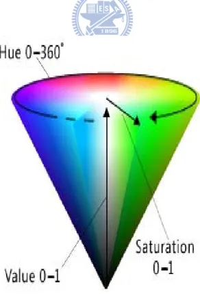
The HSV (hue, saturation and value) color space corresponds closely to the human perception of color. Conceptually, the HSV color space is a cone as shown in Fig. 2.1. Viewed from the circular side of the cone, the hues are represented by the angle of each color in the cone relative to the 0o line, which is traditionally assigned to be red. The saturation is represent as the distance from the center of the circle. Highly saturation color are on the outer edge of the cone, whereas gray tones (which have no saturation) are at the very center. The value is determined by the colors vertical position in the cone. At the point end of the cone, there is no brightness, so all colors are blacks. At the fat end of the cone are the brightness colors.
The formula of RGB transfers to HSV is defined as : ⎪ ⎪ ⎪ ⎪ ⎪ ⎩ ⎪ ⎪ ⎪ ⎪ ⎪ ⎨ ⎧ = ° + − − × ° = ° + − − × ° < = ° + − − × ° ≥ = ° + − − × ° = ° = B max min max G R G max min max R B B G R max min max B G B G R max min max B G min max H if , 240 60 if , 120 60 and if , 360 60 and if , 0 60 if , 0 ⎪ ⎩ ⎪ ⎨ ⎧ − = = otherwise , 0 if , 0 max min max max S max V = (2.16)
where max=max(R,G,B) and min =min(R,G,B).
The hue parameter is the value which represents color information without brightness. Therefore, the hue is not affected by change of the illumination brightness and direction. Although hue is the most useful attribute, there are three problems in using hue attribute for color segmentation: (1) hue is meaningless when the intensity value is very low; (2) hue is unstable when the saturation is very low; and (3) saturation is meaningless when the intensity value is very low [11]. Accordingly, Ohba et al. [14] use three criteria (intensity value, saturation, and hue) to obtain the hue value reliably.
z Intensity Threshold Value:
If V < , then Vt H =0, where V , V , and t H are an intensity value, the
16
bright enough, the color is discarded. Then, the hue value is set to a predetermined value, i.e., 0.
z Saturation Threshold Value:
If S< , then St H =0, where S, S , and t H are an saturation value, the
saturation threshold value, and a hue value, respectively. Using this equation, measured color close to gray is discarded in the image.
z Hue Threshold Value:
If 0<H <Ht or, 2π−Ht <H <2π then H =0. The range of hue
value is from 0 to 2π , and it has discontinuity at 0 and 2π . We use the phase
Chapter 3 Taking Medicine Recognition System
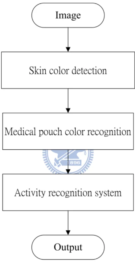
The system flowchart is illustrated in Fig. 3.1. Next, we discuss “skin color detection,” “medical pouch color recognition,” and “activity recognition system” in detail.
Image
Skin color detection
Medical pouch color recognition
Activity recognition system
Output
Fig. 3.1 The block diagram of taking medicine recognition system
Firstly, we build the grayscale value and the HSV color space background models in Scene 1, a normal view on medical pouch table. Then, our PTZ camera will zoom-in to become, a zoom-in of Scene 1, Scene 2 quickly because we do medical pouch color recognition. After the color recognition, the camera will return to Scene 1. Finally, we do activity recognition for taking medicine. Fig. 3.2 and Fig. 3.3 represent
18
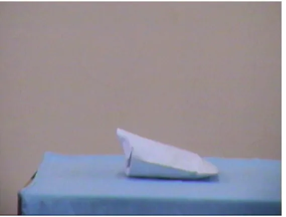
Scene 1 and Scene 2, respectively.
Fig. 3.2 Scene 1, normal view on medical pouch table
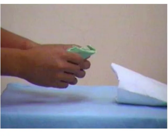
Fig. 3.3 Scene 2, zoom-in of Scene 1 and being used to recognize medical pouch’s color.
3.1 Skin Color Detection
Later, we called Scene 1 as s1 and Scene 2 as s2. In our system, we have two
zooms between s1 and s2. If the background models are ok completely, we will
have the first scene zoom that is from s1 to s2. Then, the scene was still s2 until
our system finished the medical pouch color recognition. Otherwise, we make use of skin color detection to trigger the medical pouch color recognition. Next, we will discuss the skin color detection in detail.
By skin color detection, we can discriminate that there are someone or not anyone in s2. First, the real-time image is transformed into the normalized RGB
color space by B G R R r + + = (3.1) B G R G g + + = (3.2)
According to Soriano and Martinkauppi [15], a boundary condition of skin color in the r-g plane is defined as
1452 . 0 0743 . 1 3767 . 1 ) ( =− 2 + + r r r fupper (3.3) 1766 . 0 5601 . 0 7760 . 0 ) ( =− 2 + + r r r flower (3.4)
If a pixel satisfies the following four conditions, it will be labeled as skin pixel; and further, we know there is a person in s2.
(3.5) ) ( nd ) (r a g f r f g> lower < upper (3.6) 0004 . 0 ) 33 . 0 ( ) 33 . 0 ( − 2 + − 2 ≥ g r R>G >B (3.7) (3.8) skin k G R− ≥
where kskin is a threshold.These detected skin pixels are belonged to hands because
our camera focus on subject’s hands and medical pouch. Fig. 3.4 shows an original
20
Fig. 3.4 Original image Ioriginal in s2
Next, we utilize above equations from Eqs. (3.1) - (3.8) to segment the skin
pixels in Ioriginal. Then, we can get an image Iskin from original image Ioriginal by
⎩ ⎨ ⎧ = otherwise , 0 pixel skin as detected is ) , ( if , 255 ) , (x y I x y Iskin original (3.9)
where )Ioriginal(x,y is the intensity of a pixel which is located at ( yx, ), and
) , (x y
Iskin is the segmented binary image by Eq. (3.9), as shown in Fig. 3.5.
Fig. 3.5 The binary image Iskin, in which white.
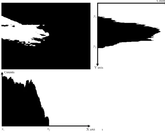
location of the subject’s hands and then the color of medical pouch can be determined. According to the binary image Iskin segmented above, we further extract the skin
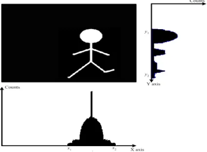
region to minimize the image size to process. Skin region extraction can be accomplished by simply a thresholding on the occupied histograms in the X and Y directions of processing image. Figure 3.6 shows an example of skin region extraction. We project the binary image Iskin and to the X and Y directions. The interested
section has higher counts in the histogram. We obtain the boundary coordinates x1, 2
x of X axis and y1, y2 of Y axis from the projection histogram. We can use these
boundary coordinates as four corners of a rectangle to locate subject’s hands, and the medical pouch as well.
22
3.2 Medical Pouch Color Recognition
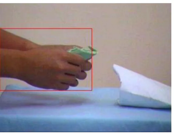
That is, it is the location of subject’s hands. According to the result of histogram of Iskin, Fig. 3.7 shows the region of subject’s hands.
Fig. 3.7 A rectangular region is detected to confine the subject’s hands
In Fig. 3.7, we find that the rectangle includes not only subject’s hands but also subject’s medical pouch. Thus, we can do medical pouch color recognition in the above rectangular region.
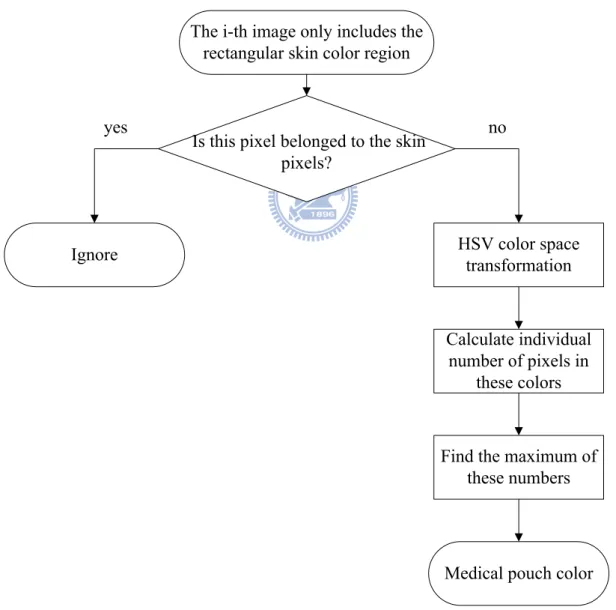
We will recognize medical pouch’s color in the HSV color space. First, we make use of Eq. (2.16) of chapter 2 to transform pixels in the hand region into the HSV color space. In order to decrease the computation, we do not transform all pixels in the region. Only the pixels not belonged to the skin pixels are transformed.
The hue value can be a reliable clue to discriminate the color of a medical pouch. The colors of our medical pouches are light red, light green and light yellow. We extract image pixels of these color medical pouches, and plot the histogram of hue component, the highly counted regions around red, green, and yellow can specify the threshold boundaries for these three colors, respectively.
belonging to the hand in the rectangular hand region are matching to the red, green, and yellow regions obtained above. The color bin with the maximal number of pixels is belonging to specify the color of medical pouch of the image. To be more reliable, we further utilize the dominant medical pouch’s color obtained in seven consecutive images to specify the final medical pouch’s color of the video clip. Fig. 3.8 shows the structure of the medical pouch color recognition.
The i-th image only includes the rectangular skin color region
Is this pixel belonged to the skin pixels? HSV color space transformation yes no Calculate individual number of pixels in these colors
Find the maximum of these numbers
Medical pouch color Ignore
24
3.3 Human Activity Recognition System
3.3.1 Object Extraction
A. Background Model
First, we only build a grayscale value background model and find out it cannot detect reliably those foreground pixel whose grayscale values close to background pixel. In order to solve this problem, we also build another background model in the HSV color space. The HSV color space corresponds closely to the human perception of color. We can have the luminance information and the chromatic information simultaneously. Hue is unreliable in some condition, so we use the three criteria (intensity value, saturation, and hue) described in Chapter 2 to obtain the hue value reliably.
In the grayscale value background model, each pixel of background scene is characterized by three statistics: minimum grayscale value ngray( yx, ), maximum grayscale value mgray( yx, ) and maximum inter-frame difference ( y, )
x
dgray of a
background video. Because these three values are statistical, we need a background video without any moving objects, for background model training. Let I be an image
frame sequence and contains N consecutive images. Iigray( yx, ) is the grayscale value of a pixel which is located at ( yx, ) in the i-th frame of I. The grayscale value background model, [mgray(x,y),ngray(x,y),dgray(x,y)], of a pixel is obtained by
{
}
{
}
{
}
⎥⎥ ⎥ ⎥ ⎦ ⎤ ⎢ ⎢ ⎢ ⎢ ⎣ ⎡ − = ⎥ ⎥ ⎥ ⎦ ⎤ ⎢ ⎢ ⎢ ⎣ ⎡ − ( , ) ) , ( max ) , ( min ) , ( max ) , ( ) , ( ) , ( 1 i y x I y x I y x I y x I y x d y x n y x m gray i gray i i gray i i gray i gray gray gray (3.10) where .i=1 ,2,... ,NIn the other hand, we build another background model with the minimum value ([ H( , ), S( , ), V( , )]
n x y n x y n x y ) and maximum value ([ H( , ), S( , ), V( , )] m x y m x y m x y ) in
each HSV domain. Then, we also record the inter-frame ratio in the brightness information and the inter-frame different in the chromatic information. Likewise, we use the same background video, for background model training. Suppose the observed
image frame sequence that contains N consecutive images. H
( )
, iI x y is the pixel’s
hue value at
( )
x,y of the i-th image frame. IiS( )
x y, is the pixel’s saturation valueat
( )
x,y of the i-th image frame. IiV( )
x y, is the pixel’s brightness value at( )
x,yof the i-th image frame. The background model of a pixel is obtained by
{
}
{
}
{
}
⎥⎥ ⎥ ⎥ ⎦ ⎤ ⎢ ⎢ ⎢ ⎢ ⎣ ⎡ − = ⎥ ⎥ ⎥ ⎦ ⎤ ⎢ ⎢ ⎢ ⎣ ⎡ − ( , ) ) , ( max ) , ( min ) , ( max ) , ( ) , ( ) , ( 1 i y x I y x I y x I y x I y x d y x n y x m H i H i i H i i H i H H H (3.11){
}
{
}
{
}
⎥⎥ ⎥ ⎥ ⎦ ⎤ ⎢ ⎢ ⎢ ⎢ ⎣ ⎡ − = ⎥ ⎥ ⎥ ⎦ ⎤ ⎢ ⎢ ⎢ ⎣ ⎡ −( , ) ) , ( max ) , ( min ) , ( max ) , ( ) , ( ) , ( 1 i y x I y x I y x I y x I y x d y x n y x m S i S i i S i i S i S S S (3.12)26
{
}
{
}
{
}
{
}
{
}
{
}
⎪ ⎪ ⎪ ⎪ ⎪ ⎪ ⎩ ⎪ ⎪ ⎪ ⎪ ⎪ ⎪ ⎨ ⎧ < ⎥ ⎥ ⎥ ⎥ ⎥ ⎥ ⎦ ⎤ ⎢ ⎢ ⎢ ⎢ ⎢ ⎢ ⎣ ⎡ ≥ ⎥ ⎥ ⎥ ⎥ ⎥ ⎥ ⎦ ⎤ ⎢ ⎢ ⎢ ⎢ ⎢ ⎢ ⎣ ⎡ = ⎥ ⎥ ⎥ ⎥ ⎥ ⎦ ⎤ ⎢ ⎢ ⎢ ⎢ ⎢ ⎣ ⎡ − − − 1 ) , ( / ) , ( if ) , ( / ) , ( max ) , ( min ) , ( max 1 ) , ( / ) , ( f i ) , ( / ) , ( max ) , ( min ) , ( max ) , ( ) , ( ) , ( 1 1 -i 1 1 i y x I y x I y x I y x I y x I y x I y x I y x I y x I y x I y x I y x I y x d y x n y x m V i V i V i V i i V i i V i V i V i V i V i i V i i V i V V V (3.13) where i=1 ,2 ,...,NB. Extraction of Foreground Object
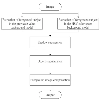
Fig. 3.9 shows the framework we apply to foreground subject extraction. Our framework of foreground subject extraction is composed of four components.
The first component is foreground subject extraction in the grayscale value and the HSV color space background models. The second component is the shadow suppression. The third component is the object segmentation. And the finally component is the foreground image compensation to recover the foreground pixels those are wrongly classified to the background.
Foreground objects can be segmented from every frame of the video stream. Each pixel of the video frame is classified to either a background or a foreground pixel by the difference between the background model and a captured image frame. First, we utilize the maximum grayscale value mgray
( )
x , , minimum grayscale value y n( )
x ,yand maximum inter-frame difference dgray
( )
x , of the grayscale value background ymodel to segment a foreground by
⎪ ⎩ ⎪ ⎨ ⎧ − > + < = otherwise , 255 ) ) , ( ( ) , ( and ) ) , ( ( ) , ( if , 0 ) , ( 1 μ μ k y x n y x I k y x m y x I y x I it gray gray t i foreground (3.14) where )It( yx,
i is the intensity of a pixel which is located at
( )
x,y , )( , 1y x I foreground
is the gray level of a pixel in binary image, μ is the median of all dgray
( )
x , , and k yis a threshold. Threshold k is determined by experiments according to difference environments. The value of k affects the amount of information retained in binary
image )1 ( ,
y x I foreground .
In the other hand, we utilize the maximum value V
(
,)
m x y , the minimum value
(
,)
V
n x y and maximum inter-frame value ratio dV
(
x y,)
of the HSV color space28 ⎪ ⎩ ⎪ ⎨ ⎧ < < = otherwise , 255 ) , ( ) , ( / ) , ( or ) , ( ) , ( / ) , ( if , 0 ) , ( 2 y x d k y x n y x I y x d k y x m y x I y x I iV V V V V V V V i foreground (3.15) where V
(
,)
iI x y is the intensity of a pixel which is located at
( )
x,y , )I2foreground(x,yis the gray level of a pixel in a binary image, k is a threshold, determined by light V
sufficiency of the scene. k will be reduced for in-sufficient light condition and V
increased otherwise.
C. Shadow Suppression
The pixels of the moving cast shadows are easily detected as the foreground pixel in normal condition. Because the shadow pixels and the object pixels share two important visual features: motion model and detectability. For this reason, the moving shadows cause object merging and object shape distortion. Therefore, we need to remove the shadow by using a shadow filter. The detail of the shadow filter is in next paragraph.
First, we discuss the shadow filter in the grayscale value. Let B( yx, ) be the background image formed by temporal median filtering, and I( yx, ) be an image of the video sequence. For each pixel ( yx, ) belonging to the foreground, consider a
3
3× template T such that xy Txy(m,n)=I(x+m,y+n), for −1≤m≤1 ,−1≤n≤1(i.e. xy
T corresponds to a neighborhood of pixel ( yx, )). Then, the NCC between
) , ( ) , ( ) , ( xy T B x y E E y x ER y x NCC = (3.16) where
∑ ∑
∑ ∑
∑ ∑
− = =− − = =− − = =− = + + = + + = 1 1 1 1 2 1 1 1 1 2 1 1 1 1 ) , ( ) , ( ) , ( ) , ( ) , ( ) , ( n m xy T n m B n m xy n m T E n y m x B y x E n m T n y m x B y x ER xy (3.17)If a pixel ( yx, ) is in a shadowed region, the NCC should be large (close to one), and
the energy ETxy of this region should be lower than the energy EB( yx, ) of the
corresponding region in the background images. There, we get
⎪⎩ ⎪ ⎨ ⎧ ≥ < = otherwise , foreground ) , ( and ) , ( shadow, ) , ( 1 NCC x y L E E x y y x S ncc Txy B (3.18) where )1( , y x
S is the shadow mask to class the pixel in the moving cast shadow, and
ncc
L is a fixed threshold. If Lncc is low, several foreground pixels may be
misclassified as shadow pixels. Otherwise, choosing a large value of Lncc, then the
actual shadow pixels may not be detected.
We know that shadow pixels have similar chromaticity, but lower brightness than the background model. Hence, we can detect the shadow from foreground subject in the HSV color space. We analyze only points belonging to possible moving object that are detected in the former step. We define another shadow mask 2
S for each ( , )x y
30 ⎪ ⎪ ⎩ ⎪ ⎪ ⎨ ⎧ < − < − < − = otherwise , foreground ) , ( ) , ( ) , ( and ) , ( ) , ( ) , ( and 0 ) , ( ) , ( if shadow, ) , ( 2 y x d k y x m y x I y x d k y x m y x I y x n y x I y x S S S S S i H H H H i V V i (3.19) where H( , ) i
I x y ,IiS( , )x y , and IiV
(
x y,)
are respectively the HSV channel of a pixellocated at
( )
x,y , and S2(x,y) is the shadow mask to class the pixel in the movingcast shadow. Values k and S k are selected threshold values used to measure the H
similarities of the hue and saturation between the background image and the current observed image. Finally, the foreground subject is defined as:
( , ) 1( , ) 2( , ) y x S y x S y x Iforeground = ∨ (3.20)
D. Object Segmentation
According to the binary image Iforeground segmented by above, we extract the
region of foreground object to minimize the image size. Foreground region extraction can be accomplished by simply introducing a threshold on the histograms in X and Y direction. Fig. 3.10 shows an example of foreground region extraction. We utilize the binary image and project it to X and Y directions. The interested section has higher counts in the histogram. We obtain the boundary coordinates x1, x2 of X axis and y1, y2
of Y axis from the projection histogram. We can use these boundary coordinates as four corners of a rectangle to extract foreground region and the size of this rectangle is adjusted to 128×96. Fig. 3.11 is the extracted foreground region.
Fig. 3.10Histogram of binary image projection in X and Y direction.
Fig. 3.11 The binary image of extracted foreground region.
E. Foreground Image Compensation
Detecting all foreground pixels and removing all shadows simultaneously are difficult. When we want to remove shadow pixels, some foreground data will be lost and this makes the foreground image be broken. Therefore, we will repair the foreground image by opening filter and closing filter.
32
3.3.2 Background Update
If we move indoor facilities, they will be detected as foreground pixels and the activity recognition will be misclassified. Therefore, we have to update background models in order to avoid above state occurring. Background models will be updated if this real-time video does not vary for a long time and there is nobody in the scene. By Eq. (3.10), we can calculate how many times the binary values remain unchanged.
⎩ ⎨ ⎧ + = = − otherwise ), , ( ) , ( ) , ( if , 1 ) , ( ) , ( 1 y x update y x I y x I y x update y x update t foreground t foreground (3.21)
where )Itforeground( yx, is the gray level of a pixel in binary image and it is located at )
,
( yx . Value update( yx, ) is a record of how many times Itforeground( yx, ) remains
unchanged.
3.3.3 Activity Template Selection
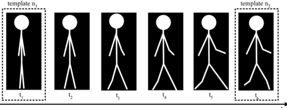
A human body is a rigid body, thus has individual natural frequency; namely, it has restriction on action speed when doing some specific actions. Because cameras usually capture image frames in a high frequency, i.e., 30 frames /sec, there are few differences between two consecutive postural image frames in a short interval. Therefore, we select some key posture frames from a sequence to describe an activity, i.e., our sample rate is 6 frames /sec. In our approach, we select one image frame, called as the essential template image, with a fixed interval instead of each image, i.e., our interval is 0.167 sec. An example is shown in Fig. 3.12. After selecting the
templates, each action is represented by several essential templates.
Fig. 3.12 One image frame is selected as template with an interval.
By eigenspace transformation (EST) and canonical space transformation (CST), these essential templates are transformed to a new space. The approximation will lose slight information of image with little differences, but it can decrease massive data dimensions. However, two similar image frames will converge to two near points in the new space that is after eigenspace and canonical space transformation. The images of similar postures done by difference people also barely converge to one point. Consequently, we select only essential templates rather than use all sequences for human activity recognition.
As described in Section 2.1, each image frame is transformed to a (c–1)-dimensional vector by EST and CST methods. Assume that there are n training models and c clusters in the system. Therefore, we have Nt templates, where Nt is
equal to n multiplied by c. Let g be a vector of template image of the j-th training i,j
model and the i-th category and t be the transformed vector of i,j g . i,j t is i,j
computed by n j c i j i j i, =H⋅g, , =1 ,2 ,L , ; =1 ,2 ,L , t (3.22)
34
where H denotes the transformation matrix combing EST and CST and n is the total
number of posture images in the i-th cluster. t is a (c–1)-dimensional vector and i,j
each dimension is supposed to be independent. Hence, t is rewritten as i,j
[
1]
T , 2 , 1 , , , , , − = c j i j i j i j i t t L t t (3.23)The transformation of each training model’s templates is treated as a mean vector. That is,
∑
= = n j j i i n 1 , 1 t μ (3.24)where i is the number of template categories. The standard deviation vector of the
m-th dimension is computed by
(
)
1 1 1 2 , − − =∑∑
= = t c i n j m i m j i m N t μ σ (3.25) where 1m=1 ,2,K ,c− .3.3.4 Construction of Fuzzy Rules form Video Stream
For human activity classification, transitional relationships of postures in a temporal sequence are important information. Human’s actions may have similar postures in two different activity sequences, and therefore only using one image frame to classify the action is not sufficient. For example, the actions of “jumping” and “crouching” both have the same postures called common states as shown in Fig. 3.13. Besides, the posture sequence of each activity is dissimilar in different people.
Hence, we propose a method which not only combines temporal sequence information for recognition but also is tolerant to variations of different people. We use the fuzzy rule-base approach to design our system. The fuzzy rule-base approach also has been proposed in gesture recognition in [16]; it has ability to absorb data difference by learning.
36
We use the membership function to represent the feature’s possibility of each cluster. We choose the Gaussian type membership function to represent the features because the Gaussian type membership function can reflect the similarity via the first order and second order statistics of clusters and is differentiable.
Firstly, when the k-th training image frame xk is inputted, the feature vector ak is
extracted by
ak =Hxk. (3.26)
where H denotes the transformation matrix combing EST and CST. As the same as ti,j
in Eq.(3.21), ak can be rewritten as
=
[
1 , 2, , c−1]
T. k k k k a a L a a (3.27)If we suppose the dimensions of the feature vectors are independent, a local measure of similarity between the training vector and each template vectors can be computed. Let Σ denote the covariance matrix of all essential template vectors and Ci
denote the i-th class of essential templates. The membership function is given by
⎪⎭ ⎪ ⎬ ⎫ ⎪⎩ ⎪ ⎨ ⎧ ⎥ ⎥ ⎦ ⎤ ⎢ ⎢ ⎣ ⎡ − − = ⎥⎦ ⎤ ⎢⎣ ⎡− − − = =
∏
−∑
= − = − − 1 1 1 1 2 2 , j 1 2 1 2 1 , ) ( 2 1 exp 2 1 max arg ) ( ) ( 2 1 exp ) 2 ( 1 ) ( M c m c m m m j i m k m T c i k i a C r σ μ σ π π μ a Σ μ a Σ a k k k(3.28)
where j is the training model number. ri,k denotes the grade of membership function
in category i of the k-th image frame. Besides, we can obtain which category each image belongs to by k i k r p , i max arg = (3.29)
The membership function describes the probability of which one it is like most. But it just contains the information of a single image. Hence, we collect three images to form a basis for temporal information.
Assume we have c linguistic labels, each linguistic label represent a category of essential template. Each image frame can be represented by one of these c linguistic labels. Here, we combine three contiguous images to a group( , , )I I I1 2 3 and the
interval of itself and next is 0.167 sec. The transformation of the image group can
form a feature vector [a a a .There are c1, 2, ]3 3 combinations of the feature vector. Each combination represents the possible transition states of the three images. We use Eqs. (3.26) and (3.27) to class each image frame. Hence, we can represent the feature vector (
[
a1,a2,a3]
) by linguistic label sequence([
P1,P2,P3]
). An image sequencewith linguistic label sequence is associated with its output of corresponding activity. As developed by Wang and Mendel [17], fuzzy rules can be generated by learning from examples. Such image sequence constitutes an input-output pair to be learned in the fuzzy rule base. In this setting, the generated rules are a series of associations of the form
“IF antecedent conditions hold, THEN consequent conditions hold.”
38
antecedent conditions are connected by “AND.” For example, an image sequence, its transformations of image 1, image 2, image 3 and belonging categories being concatenated as vector format, is given by
[
P1,P2,P3;D1]
(3.30)
Suppose that Image 1, Image2 and Image 3 belong to key posture 1, key posture 2 and key posture 3 respectively. Therefore, we assign the image sequences, whose feature vector is [ 1 1 a , 1 2 a , 1 3
a ], to the linguistic labels Posture 1, Posture 2 and Posture 3 respectively. Finally, according to the feature-target association implies this image sequence to support the rule of
Rule 1. IF the activity’s I1 is P11 AND its I2 is P AND its 21 I is 3 P , 31
THEN the activity is D1. (3.31)
After the learning steps of action video, some rules that obtained enough member of supporting fire strength may be representative to describe an action in video. In this thesis, a rule with at least four supporting input image frames is selected and compiled to constitute the knowledge rule base of our action recognition system. During the training of image sequences, we can compute the mean and standard deviation of each pre-defined activity.
3.3.5 Classification algorithm
After constructing the rule base, we can grade the input image sequence with each fuzzy rule by grade of membership function. Let Σ denote the covariance matrix of all essential template vectors, Ci denote the i-th class of essential templates and sk
denote the image frame transformed by EST and CST. The membership function is given by ⎪⎭ ⎪ ⎬ ⎫ ⎪⎩ ⎪ ⎨ ⎧ ⎥ ⎥ ⎦ ⎤ ⎢ ⎢ ⎣ ⎡ − − = ⎥⎦ ⎤ ⎢⎣ ⎡− − − = =
∏
−∑
= − = − − 1 1 1 1 2 2 , j 1 2 1 2 1 , ) ( 2 1 exp 2 1 max arg ) ( ) ( 2 1 exp ) 2 ( 1 ) ( M c m c m m m j i m k m T c i k i s C s r σ μ σ π π μ s Σ μ s Σ k k k(3.32)
where j is the training model number. ri,k denotes the grade of membership function
in category i of the k-th image frame. σ is the standard deviation of all essential templates. These membership functions are just the results of one image frame. Therefore, we use two transformed vector of passed image frames, which are called
2 − k
a and ak−1. Then, we set these three vectors as a feature vector [ak−2,ak−1,a ] k
and compute the membership functions of them respectively.
In order to calculate the similarity between image sequence and each postural sequence in the training data base, we take out the membership functions rk−2 n,1,
2
, 1 n k
r− and rk,n3 which are corresponding to the three category of linguistic labels, 1
Pn , Pn2 and Pn3, in the rule and have been calculated by Eq. (3.29). The summation
of rk−2 n,1, rk−1 n,2 and rk,n3 is the similarity between current image sequence and the
postural sequence of this rule. We can obtain the similarity related to all fuzzy rules of training data base in the same manner. The rule, which has the highest value of similarity, is selected.
40
Chapter 4 Experimental Results
In our experiment, we tested our system on videos taken by PTZ camera. We took the video in our laboratory at the 5th Engineering Building in NCTU campus. The light source is fluorescent lamp and is stable. The background is not complex and we equip a table in the scene. The camera is set up at a fixed location and kept stationary. This camera has a frame rate of thirty frames per second and image resolution is 320 240× pixels. Scene 1 is a normal view on medical pouch table, and Scene 2 is the zoom-in of Scene 1. Fig. 4.1 and Fig. 4.2 represent Scene 1 and Scene 2, respectively.
Fig. 4.1 Scene 1, normal view on medical pouch table
Fig. 4.2 Scene 2, zoom-in of Scene 1 and being used to recognize medical pouch’s color.
In our recognition systems, we have eight training actions: “walking from right to left,” “walking from left to right,” “walking straightly,” “reading ,” “using computer,” “sleeping,” “taking medicine,” and “picking up.”
4.1 Skin Color Detection and Medical Pouch Color Detection
4.1.1 Skin Color Detection
Skin color detection is used for segmenting the object’s hands. If we segment the skin region more precisely, we can extract object’s hands more correctly. A threshold
skin
k is applied in Eq. (3.8) described in Section 3.1 to obtain binary image B
( )
x ,y .The value of kskin is chosen by experiment and varies with different environments.
Hence, we ran a series of experiments to determine the optical threshold kskin and the
corresponding binary images are shown in Fig. 4.3. The threshold kskin=45 was
adopted in our experiment.
Hand region is extracted from binary image B
( )
x ,y in order to minimize thesize of images. Hand region extraction is accomplished by simply taking a threshold along X and Y directions. Fig. 4.4 shows an example of hand region extraction. Fig. 4.4(a) is a image frame of the video stream. Figure 4.4(b) is the binary image after performing background model analysis. Figures 4.4(c) and 4.4(d) show the projection of Fig. 4.4(b) onto the X and Y directions, respectively. We can find the boundary coordinates of the X and Y directions by observing the projection histogram. We used these boundary coordinates to define a rectangle to extract foreground region from Fig. 4.4(b). Fig. 4.4(e) is the extracted foreground region.
42
(a) (b)
(c) (d)
(e) (f)
Fig. 4.3 Example of skin color detection at different threshold, kskin, values. (a) An
(a) (b)
(c) (d)
(e)
Fig. 4.4 An example of hand region extraction. (a) An image frame, (b) binary image after skin color analysis, (c) projection of (b) onto X direction, (d) projection of (b) onto Y direction, (e) hand region extracted.
44
4.1.2 Medical Pouch Color Detection
For medical pouch color detection, we have to analyse the hue component of red, green, and yellow. Thus, we use three hundred 25×25images for each color, respectively. First, we plot the histogram of hue component by using all the above images. Then, we eliminate the first 5% and the last 5% in these data, and get a new range for each color. For red, its hue component value is between 296 and 317. For green, its hue component value is between 114 and 169. For yellow, its hue component value is between 37 and 58. We show some images in these analytic data in Fig. 4.5. These histogram plots are shown Figs. 4.6 – 4.8.
(a)
(b)
(c)
Fig. 4.5 Some pouch’s color images in analytic phase. (a) red data, (b) green data, (c)yellow data.
Fig. 4.6 Histogram plot of hue component in the red data.
Fig. 4.7 Histogram plot of hue component in the green data.
-50 0 50 100 150 200 250 300 350 400 0 1 2 3 4 5 6 7 8x 10 4 -500 0 50 100 150 200 250 300 350 400 1 2 3 4 5 6x 10 4