國
立
交
通
大
學
企業管理碩士學程
碩
士
論
文
數量彈性與二次訂購契約之供應鏈效益分析
SUPPLY CHAIN EFFECTS OF QUANTITY-FLEXIBILITY
CONTRACT AND DOUBLE-ORDERING CONTRACT
研 究 生:藍心如
指導教授:韓復華 教授
National Chiao Tung University
Global MBA Program
Thesis
Supply Chain Effects of Quantity-Flexibility Contract and
Double-Ordering Contract
Student: Hsin-Ju Lan
Advisor: Prof. Anthony F. Han
Supply Chain Effects of Quantity-Flexibility Contract and
Double-Ordering Contract
研 究 生:藍心如
Student: Hsin-Ju Lan
指導教授:韓復華
Advisor: Dr. Anthony F. Han
國 立 交 通 大 學
企業管理碩士學程
碩 士 論 文
A Thesis
Submitted to Global MBA Program College of Management National Chiao Tung University in partial Fulfillment of the Requirements
for the Degree of Master
in
Global Master of Business Administration
June 2010
Hsinchu, Taiwan, Republic of China
-i-
Supply Chain Effects of Quantity-Flexibility Contract and
Double-Ordering Contract
Student: Hsin-Ju Lan
Advisor: Dr. Anthony F. Han
Global Master of Business Administration
National Chiao Tung University
ABSTRACT
Recently, the improvement of manufacturing technology and information technology accelerate the development of supply chain management. So that coordination between supply chain members becomes more and more important. Supply chain contracts for collaborating the relationship between supply chain members thus becomes a powerful tool to improve the competitiveness of the whole supply chain.
This thesis focuses on two unconventional supply chain contracts, i.e. quantity-flexibility contract (QFC) and double-ordering contract (DOC). Using simulation analysis, we found that both QFC and DOC can increase the supply chain profitability under certain circumstances. The total supply chain profit effect seems to be more significant for QFC than that for DOC. While the QFC tends to make supply chain gains in all cases tested, the gains tend to increase as the product margin decreases. However, we found that the share of the profit is not fairly distributed. For both QFC and DOC, the buyer tends to take most of the gains and the supplier tends to suffer a loss. Therefore, for sustainable development of supply chain contract relations, an appropriate reward system to the supplier is critical. This provides an important subject for future research.
-ii-
Acknowledgements
The completion of this research would not have been possible without the help and support from many people. First of all, I would like express my greatest gratitude to my advisor, Dr. Anthony F. Han, for his expertise, guidance and support from the initial to the final of this research. I also want to thanks the committee members of my oral defense, Dr. Ming-Jong Yao and Dr. Yuh-Jen Cho, for giving me their valuable comments on my study. My gratitude extends to Dr. Ka Io Wong who helped me to review my thesis draft and gave me good comments.
Next, I would like to thanks to all the professors and my fellow GMBA classmates. I am very cherishing the time we have shared in last two years. Because of you, my school life becomes sparkling.
Further, I am thankful to Ms. Karen Wu and HANA Microelectronics (BKK) Ltd., Co. and coworkers in HANA, to help me accomplish my overseas internship. It was a memorable and a precious experience in my life.
Finally, my deepest appreciation goes to my friends and family for their kindly support and encouragement in this two-year study.
-iii-
Supply Chain Effects of Quantity-Flexibility Contract and
Double-Ordering Contract
Table of Contents
Abstract ... i
Acknowledgements ... ii
Table of Contents ... iii
List of Tables ... v
List of Figures ... vi
I. Introduction ... 1
1.1 Research Motivation ... 1
1.2 Research Scope ... 2
1.3 Methodology and Framework ... 2
II. Literature Review ... 4
2.1 Value Chain and Supply Chain ... 4
2.2 Supply Chain Management ... 5
2.3 EOQ and Service Level ... 6
2.4 Supply Chain Contracts ... 8
2.4.1 Quantity-Flexibility Contract ... 10
2.4.2 Double-Ordering Contract ... 13
2.5 Conclusion ... 15
III. Analysis of Quantity-Flexibility Contract ... 16
3.1 Quantity-Flexibility Contract Model Formulation ... 16
3.2 Experimental Design ... 18
3.3 Simulation Modeling (Excel) ... 20
-iv-
3.5 Sensitivity Analysis and Discussion ... 24
IV. Analysis of Double-Ordering Contract ... 28
4.1 Single Order Contract Model Formulation ... 28
4.2 Double-Ordering Contract Model Formulation ... 29
4.3 Experimental Design ... 32
4.4 Simulation Modeling (Excel) ... 34
4.5 Simulation Results ... 35
4.6 Sensitivity Analysis and Discussion ... 38
V. Conclusion ... 41
5.1 Research Summary... 41
5.2 Extension for Future Research ... 42
Reference... 44
Appendix A QFC Simulation Results ... 46
v
List of Tables
Table 1 Parameters Setting of QFC Simulation Models ... 19
Table 2 Simulation Scenarios of QFC ... 19
Table 3 Optimal OF for Different Flexibility (Buyer) ... 22
Table 4 Simulation Scenarios of QFC Sensitivity Analysis ... 24
Table 5 Parameters Setting of SOC and DOC Simulation Model ... 33
Table 6 Simulation Scenarios of SOC and DOC ... 33
vi
List of Figures
Figure 1 Research Framework ... 3
Figure 2 Value Chain ... 4
Figure 3 Buyer’s Profit ... 22
Figure 4 Supplier’s Profit ... 23
Figure 5 Total Supply Chain Profit ... 23
Figure 6 Buyer’s Profit (α = β=0 & α = β=0.1) ... 26
Figure 7 Supplier’s Profit (α = β=0 & α = β=0.1) ... 26
Figure 8 Total Supply Chain Profit (α = β=0 & α = β=0.1) ... 27
Figure 9 Timeline sketch of DOC ... 30
Figure 10 Buyer’s Profit ... 36
Figure 11 Supplier’s Profit ... 37
Figure 12 Total Supply Chain Profit ... 37
Figure 13 Effect of Buyer’s Profit (k=1/4) ... 39
Figure 14 Effect of Supplier’s Profit (k=1/4) ... 40
Figure 15 Effect of Total Supply Chain Profit (k=1/4) ... 40
1
I. Introduction
1.1 Research Motivation
In this competitive market environment, every company is eager to find out the effective mechanism in order to reduce their cost and satisfy customers. Although the ampler goods on hand will come out the better customer satisfaction, it will also increase cost. In addition, as we know, material cost fluctuates rapidly these few years. Thus, inventory management becomes a significant issue for a business.
It is very important in particular for the seasonal products which are characterized by limited selling period and shorter PLC (product life cycle). Due to the salvage value of the seasonal products decreases extremely after the sales period. Therefore, if there are a lot of inventories in the end of the sales season, enterprise’s profit will be eroded. In other words, if we can reduce demand uncertainty and forecast accurately, which can place order with precise quantities in order to meet both the higher CSL (customer service level) and the lower inventory cost, we can increase the profit.
Chopra and Meindl [1] stated that Quick Response (QR) is a set of actions a supply chain takes to reduce the replenishment lead time so that multiple orders may be placed in the selling season. Supply chain managers are able to improve their forecast accuracy as lead times decrease, which allows them to better match supply with demand and increase supply chain profitability.
Besides the improvement of technology, coordination between members in supply chain is very important. As Cachon [2] mentioned, optimal supply chain performance requires the execution of a precise set of actions. Unfortunately, those actions are not always in the best interest of the members in the supply chain, i.e., the supply chain members are primarily concerned with optimizing their own objectives, and that self-serving focus often results in poor performance. However, optimal performance is
2
achievable if the firms coordinate by contracting on a set of transfer payments such that each firm’s objective becomes aligned with the supply chain’s objective. Hence, how does the supply chain coordinate in order to maximize the whole supply chain profit is another important issue faced by businesses.
Supply chain contracts have been developed to coordinate between buyers and suppliers in supply chain. They not only specify the price, volums, delivery etc., but also help to optimize the supply chain performance particularly.
As mentioned above, reducing demand uncertainty is quiet important for the seasonal product. If the supplier offer more flexible ordering terms for reducing demand uncertainty, the buyer would be encouraged to order more quantity to meet the
customer’s need, the overall supply chain profit will increase.
Quantity-flexibility contracts(QFC) and Double-ordering contract(DOC) provide the buyer to order much flexibly. These contracts allow the buyers adjust their order or provide one more ordering opportunity after observing market demand. Thus, our study is to understand the impact of QFC and DOC on the buyer, the supplier and the total supply chain.
1.2 Research Scope
Therefore, our research scopes are as listed follows.
(1) To analyze the effects of supply chain profit with and without QFC and DOC respectively.
(2) To analyze the impact of supply chain profit sharing on each supply chain member with and without QFC and DOC respectively.
(3) And also to find out some managerial implications of supply chain contracts for supply chain manager.
3
There are a lot of researches relative to our topic which brought up many models in order to find out the solutions that can coordinate the parties in the supply chain and optimize the supply chain profit.
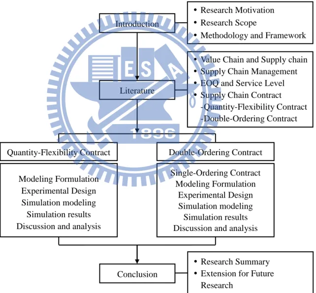
Rather than develop a model, our study is using Microsoft Excel to simulate different scenarios which is designed in terms of Quantity-flexibility contract (QFC) and Double-ordering contract (DOC) and to analyze the effect of the supply chain contracts and related implication. Figure 1 shows the framework of this research.
Figure 1 Research Framework Quantity-Flexibility Contract
Modeling Formulation Experimental Design Simulation modeling Simulation results Discussion and analysis
Double-Ordering Contract Single-Ordering Contract Modeling Formulation Experimental Design Simulation modeling Simulation results Discussion and analysis
Conclusion
Research Summary Extension for Future
Research
Research Motivation Research Scope
Methodology and Framework Introduction
Literature Review
Value Chain and Supply chain Supply Chain Management EOQ and Service Level Supply Chain Contract
- Quantity-Flexibility Contract - Double-Ordering Contract
4
II. Literature Review
2.1 Value Chain and Supply Chain
Michael Porter [3] introduced a value chain model that helps to analyze specific activities that is creating value competitive advantages. The value chain categorizes the generic value-adding activities of an organization. The "primary activities" include: inbound logistics, operations (production), outbound logistics, marketing and sales (demand), and services (maintenance). The "support activities" include: administrative infrastructure management, human resource management, technology (R&D), and procurement. The costs and value drivers are identified for each value activity.
Figure 2 Value Chain
(Source: Michael Porter: Competitive Advantage, 1985)
Martin Christopher [4] defined supply chain is “the network of organizations that are involved in different processed and activities, through upstream and downstream linkages, that produce value in the form of products and service to the ultimate customer.”
5
Chopra and Meindl [1] stated that a supply chain consists of all parties involved, directly or indirectly, in fulfilling a customer request. The supply chain includes not only the manufacturer and suppliers, but also transporters, warehouses, retailers, and even customers themselves. Within each organization, such as a manufacturer, the supply chain includes all functions involved in receiving and filling a customer request.
2.2 Supply Chain Management
Council of Supply Chain Management Professionals (CSCMP) defined that Supply chain management encompasses the planning and management of all activities involved in sourcing and procurement, conversion, and all logistics management activities. Importantly, it also includes coordination and collaboration with channel partners, which can be suppliers, intermediaries, third party service providers, and customers. In essence, supply chain management integrates supply and demand management within and across companies.
Another definition is provided by the APICS Dictionary when it defined Supply Chain Management as the "design, planning, execution, control, and monitoring of supply chain activities with the objective of creating net value, building a competitive infrastructure, leveraging worldwide logistics, synchronizing supply with demand, and measuring performance globally."
Chopra and Meindl [1] defined that supply chain management involves the management of supply chain assets and product, information, and fund flows to maximize total supply chain profitability.
Simchi-Levi et al. [5] defined that supply chain management is a set of approaches utilized to efficiently integrate suppliers, manufacturers, warehouses, and stores, so that merchandise is produced and distributed at the right quantities, to the right locations, and at the right time, in order to minimize systemwide costs while satisfying service
6
level requirement.
Stadtler [6] defined supply chain management as the task of integrating
organizational units along a supply chain and coordinating material, information and financial flows in order to fulfill (ultimate) customer demands with the aim of improving the competitiveness of a supply chain as a whole.
2.3 EOQ and Service Level
Undoubtedly, inventory control is a significant issue in supply chain management. The goal of effective inventory management in the supply chain is to have correct inventory at the right place at the right time to minimize system costs while satisfying customer service level[5]. In order to meet the goal, optimize the order quantity is one of the critical issues in inventory management. Here we introduce the economic order quantity model and service level that have been used to control the inventory
availability.
Economic order quantity model (EOQ model) is a level of inventory that minimize the holding cost and ordering cost.
Harris[7] first introduced the economic order quantity model which is the trade-offs between ordering and storage cost. The model assumes the following,
(1) Demand, D, is constant.
(2) Order quantities Q are fixed per order.
(3) A fixed setup cost, K, is incurred while placing an order. (4) A unit holding cost, h, is accrued when the inventory is held. (5) The lead time is zero.
(6) Initial inventory is zero.
(7) The planning horizon is infinite.
7
(9) The goal of this model is to find the optimal order policy that minimizes annual purchasing and holding costs while meeting all demands.
Q* = (1)
Service level is the probability of not having a stockout in an order. Baker [8] demonstrates the limitations of this notion and calls for analysis of the relation between end-item service levels and component safety stocks when there are both unique and common component. Baker et al.[9] analyze a two-product, two-level model for the effects of commonality on component safety stock. They posed a constrained
optimization problem which involves minimizing total component safety stock subject to a service level requirement.
Schneider and Ringquest [10] presented an analytic approximation for computing (s, S) policies under a specific service level. This model has been developed for a periodic review, single-item system which assumes a fixed ordering cost, linear holding costs, replenishment lead time is fixed and unfilled demand is backlogged.
Chen and Krass [11] investigated the inventory models in which the stockout cost is replaced by a minimal service level constraint (SLC) that requires a certain level of service to be met in every period. The minimal service level approach has the virtue of simplifying the computation of an optimal ordering policy, because the optimal reorder level solely determined by the minimal SLC and demand distributions. It’s found that above a certain “critical” service level, the optimal (s, S) policy collapses to a simple base-stock or order-up-to level policy, which is independent on the cost parameter.
Bollapragada et al.[12] considered stock positioning in a pure assembly system controlled using installation base-stock policies.They proposed a decomposition approach that uses an internal service level to independently determine near-optimal stock levels for each component. Compared with the current practice, this approach has
8
the potential to reduce that safety-stock cost by as much as 30%.
Since our research is focus on the newsboy product, which has short life cycle and the left over product should dispose of after sales period. So that the optimal order quantities should consider the trade-off of the stockout and shortage and might not fully satisfy the customer’s needs. Thus, here we choose critical fractile as the reference of deciding the ordering quantities instead of EOQ.
2.4 Supply Chain Contracts
Chopra and Meindl [1] stated that a supply chain contract specifies parameters governing the buyer-supplier relationship. Contracts should be designed to facilitate desirable supply chain outcomes and minimize actions that hurt performance. Ideally, a contract should be structured to increase the firm’s profits and supply chain profits, discourage information distortion, and offer incentives to the supplier to improve performance along key dimensions. They classified the supply chain contracts into the following categories and discussed contracts in these categories respectively.
(1) Contracts for product availability and supply chain profits (i) Buyback or returns contracts
(ii) Revenue-sharing contracts (iii) Quantity flexibility contracts
(2) Contracts to coordinate supply chain costs (i) Quantity discounts contracts
(ii) Contracts to increase agent effort (iii) Two-part tariffs
(iv) Threshold contracts
(3) Contracts to induce performance improvement (i) Shared-savings contracts
9
Simchi-Levi et al. [5] classified supply chain contracts into different components as follows,
(1) Strategic components
(i) Buyback contracts mean that the seller agrees to buy back unsold goods from the buyer for some agreed-upon price higher than the salvage value.
(ii) Revenue-sharing contracts mean that the buyer shares some of its revenue with the seller, in return for a discount on the wholesale price. (iii) Quantity-flexibility contracts mean that the supplier provides full
refund for returned (unsold) items as long as the number of returns is no larger than a certain quantity.
(iv) Sales rebate contracts provide a direct incentive to the retailer to increase sales by means of a rebate paid by the supplier for any item sold above a certain quantity.
(2) Contracts for make-to-stock/make-to-order supply chains
(i) Pay-back contracts are that the buyer agrees to pay some agreed-upon price for any unit produced by the manufacturer but not purchased by the distributor.
(ii) Cost-sharing contracts are that the buyer shares some of the
production cost with the manufacturer, in return for a discount on the wholesale price.
(3) Contracts with asymmetric information
(i) Capacity reservation contracts are manufacturer pays to reserve a certain level of capacity with the supplier.
10
purchase price for firms’ orders placed prior to building capacity and a different price for any additional order placed when demand is realized.
(4) Contracts for nonstrategic components
(i) Long-Term contracts, also called forward or fixed commitment contracts, specify a fixed amount of supply to be delivered at some point in the future; the supplier and the buyer agree on both the price and the quantity to be delivered to the buyer.
(ii) Flexible, or option, contracts are that the buyer prepays a relatively small fraction of the product price upfront, in return for a commitment from the supplier to reserve capacity up to a certain level.
(iii) Spot purchase contracts mean that buyers look for additional supply in the open market.
(iv) Portfolio contracts mean that buyers sign multiple contracts at the same time in order to optimize their expected profit and reduce their risk.
2.4.1 Quantity-Flexibility Contract
The buyer should place an order with fixed quantities before sales season begins, however, when demand realized may higher or lower than order quantity, the buyer may suffer understock or overstock. Quantity-flexibility contract, QFC, is that the supplier allows the buyer to increase or reduce the initial order quantity to an agreed level after the buyer observed market demand.
Quantity-flexibility contracts define terms under which the quantity a retailer ultimately orders from the manufacturer may deviate from a previous planning estimate [13]. Quantity-flexibility contract has been a common practice in the electronic industry
11
since 1980s and used by Sun Microsystems, Nippon Otis, Solectron, IBM, HP, and Compaq, etc. [14]. Backup agreement have been used by Anne Klein, Finity, DKNY, Liz Claiborne, and Catco in the apparel industry [15]. It stated that, if a retailer commits to a number of units for the season, the manufacturer will hold back a fraction of the commitment and the retailer can order up to this backup quantity at the original price after observing early demand.
Eppen and Iyer [15] focused on backup agreement between a catalog company and manufacturers. A backup agreement states that, if the catalog company commits to a number of units for the season, the manufacturer holds back a constant fraction ρ of the commitment Q and delivers the remaining units (1- ρ) Q at the beginning of the selling season. After observing early demand, the catalog company can order back to this backup a quantity for the original purchase cost and receive quick delivery but will pay penalty p for any of the backup units it does not buy. This research is from the
manufacturer’s perspective. The results indicate that backup agreements can have a substantial impact on expected profits and may result in an increase in the committed quantity. Also, these arrangements may maintain the manufacturer’s expected profit for a wide range of parameters.
Tsay [14] stated that quantity flexibility contracts under rolling horizon planning are efficient coordination schemes to balance the risk of each side. The objective of this paper is to present an analytical model for these contracts, characterize the structure of the optimal policies for buyers, and develop solution methodologies that allow buyers to determine ordering quantities which minimize their expected total cost per period.
Tsay and Lovejoy [16] discussed a quantity flexibility contract under a
rolling-horizon planning. In the study, it stipulates a maximum percentage revision each element of the period-by-period replenishment schedule is allowed per planning
12
iteration. This paper develops rigorous conclusions about the behavioral consequences of quantity-flexibility contracts and addresses about the implications for the
performance and design of supply chains with linkages possessing this structure. Issues explored include the impact of system flexibility on inventory characteristics and the patterns by which forecast and order variability propagate along the supply chain.
Barnes-Shuster et al. [17] investigated the role of options in a single-buyer single-supplier system with correlated demand. The buyer orders Qi units at a unit
wholesale price of ci to be delivered at the beginning of period. In addition, the buyer
purchases M options at a unit option price of co. In period two, he may choose to
exercise m≦M options at a per unit exercise price of ce. In this research, they illustrate
how options provide flexibility to a buyer to respond to market changes in the second period. They also study the implications of such arrangements between a buyer and a supplier for coordination of the channel.
Chopra and Meindl [1] applied simulation to evaluate the impact of
quantity-flexibility contract and observe that the amount ordered by the buyer is more in line with actual demand, resulting in higher profits for the supply chain. For the supplier, the quantity-flexibility contract makes sense if it has flexible capacity that can be used to produce at least the uncertain part of the order after the buyer has decided on the modification. A quantity-flexibility contract is also very effective if the supplier is selling to multiple buyers with independent demand. In addition, as the supplier increases the wholesale price, it is optimal for it to offer greater quantity flexibility to the buyer.
In our study, we apply simulation models to analyze the impact of
Quantity-flexibility contract which is extending from Chopra and Meindl’s basic proposition. The buyer is allowed to either increase α percentage or decrease β
13
percentage of initial ordering after observing demand but before the selling season. In addition, we also consider about the unit price will be stepwise with flexibility while the order quantity is increase.
2.4.2 Double-Ordering Contract
The classical single period problem assumes that the product can only be ordered once for the beginning of the sales period. But in practice, since the technology
improvement and the coordinations between supply chain members, many single-period product can have more replenishment opportunities later in the sales period. Thus, more and more researchers studied the newsboy problems with multi-ordering opportunities. Double-ordering contract, DOC, is that the supplier allows the buyer break up the purchase of the entire season into two orders.The first order is placed before the start of the sales season. Once the sales start, the buyer observes demand and places a second order. The quantity of the second order is different from the order-up-to level for the latter sales period and the remaining inventory after the earlier sales period. After the entire sales period, the left over products will be disposed.
Fisher and Roman [18] studied a QR system that made full use of early sale records to reduce the uncertainty on customer demand. They analyzed the ordering policy with the mathematical model for a single-period product under QR system, and developed a method to estimate the demand distribution.
Iyer and Bergen [19] studied how a manufacturer-retailer channel impacts choices of production and marketing variables under QR in the apparel industry. They build formal models of the inventory decisions of manufacturers and retailers both before and after QR. The results show that QR policy always improved the system performance. However, QR may not always make both manufacturers and retailers better off. Both parties are required to undertake actions to make all parties improve.
14
Lau and Lau [20] considered that a single-period newsboy type product may be ordered or produced twice during a season/period. In this paper, it allows a reorder during mid-season after the early-season demand has been observed, and this reorder arrives after a given lead time. The demand distributions during the various portions of the season may have very general distribution forms; also, the late-season and
early-season demands may be dependent. The result indicates that the reorder
opportunity can improve profits considerably as long as the product's profit margin is not very high.
Extending from the research in 1997, Lau and Lau [21] consider a non-negligible set-up cost for second order and state the solutions of how much quantity to order initially, when to place a second order and for what quantity.
Choi et al. [22] investigated an optimal two-stage ordering policy for seasonal products. In this study, market information is collected at the first stage and is used to update the demand forecast at the second stage by using Bayesian approach. There are two single-stage ordering policy. Both can place one order before sales season. By comparing with the optimal two-stage ordering policy and the two single-stage ordering policies which can both place one order before sales season, the results show that average profit generated by optimal two-stage policy are always larger than the average profit generated by corresponding one-stage policies. The earlier the order point, the higher the demand uncertain.
Chopra and Meindl [1] used simulation method to compare single order strategy with double order strategy and observe three important consequences of being able to place a second order in the season:
(1) The expected total quantity ordered during the season with two orders is less than that with a single order for the same cycle service level. In other
15
words, it is possible to provide the same level of product availability to the customer with less inventory if a second, follow-up order is allowed in the sales season.
(2) The average overstock to be disposed of at the end of the sales season is less if two orders are allowed.
(3) The profits are higher when a second order is allowed during the sales season.
In our study, we analyze about the effect of Double-ordering contract extending from Chopra and Meindl’s simulation analysis. We concern about different information accuracy for the second order with different standard deviation (σ) to find out the impact of information updated for the second order. And also the impact of buyer’s service level with Double-ordering contract.
2.5 Conclusion
The researches mentioned above are profound with complicated models. Our study applies an uncomplicated formulas and a liable tool to analyze the effect of QFC and DOC and provide the managers a simple and clear analysis and perspectives.
16
III. Analysis of Quantity-Flexibility Contract
This chapter analyzes the effect of the quantity-flexibility contract. We first
introduce the property and formulation of QFC in our study, and then state the design of our simulation experiment in section 3.2. The following section 3.3 introduce the steps of our simulation models. After that we indicate our simulation results in section 3.4. At the end of this chapter, we propose the sensitivity analysis of our QFC simulation model and discusses the results in section 3.5.
3.1 Quantity-Flexibility Contract Model Formulation
Quantity-flexibility contracts(QFC) are common used in the electronics and computer industry. However, Benetton has also used QFC with its retailer to increase supply chain profir successfully. For example, its retailers are required to place an order for 100 sweather each in red, blue, and yellow seven months before delivery. The retailer may alter up to 30 percent of the quantity ordered in any color and assign it to another color. The aggregate order can not be adjusted at this stage. After the start of the sales season, the retailer is allowed to order up to 10 percent of the its previous order in any color. Potentially, the retailer can increase the aggregate quantity ordered by up to 10 percent across all colors and of about 40 percent for individual colors. This results in a better matching of supply and demand at a lower cost than without this contract, and allows both the retailer and Benetton to increase their profits. [1]
In this chapter, we consider a single supplier and a single buyer. The buyer placed a QFC order to the supplier.
Unlike conventional fixed quantity contract, for QFC when the buyer orders OF
units, the realized contract quantity can be in the range of (1 + α) OFand (1 – β) OF,
depending on the market demand observed closer to the point of sales. The parameters α and β represent the downscale and upscale flexibility of the supplier respectively.
17
The buyer orders OF units. After observing the market demand at the beginning of
sales season, the supplier commits to provide QF = (1 + α) OF units, whereas the buyer
is committed to buy at least qF = (1 – β) OF units from the supplier. Both α and β are
between 0 and 1. So that the buyer can purchase XF units which is from qF to QF units,
depending on the demand it observes. However, considering the additional cost of fulfilling buyer’s need immediately, when the actual order XF is larger than his or her
initial order OF, the supplier’s production cost will increase by the upscale flexibility of
the supplier, α.
To write more detailed QFC model formulation, we now define the following notations.
OF Initial order quantity by buyer
α Upscale flexibility of the supplier β Downscale flexibility of the supplier pF Selling price per unit
cF Wholesale price per unit.
mF Production cost per unit.
sF The buyer’s salvage value per unit. pF> cF> mF> sF >0
Cost of overstocking by one unit, = cF - sF
Cost of understocking by one unit, = pF - cF
Supplier profit Buyer profit Total profit
The formulas of our QFC simulation model are described as follows. The upper bound of QFC order quantity is
18
The lower bound of QFC order quantity is
qF = (1 – β) OF (3)
Actual market demand is normally distributed D~ N( , ) and DF is the realized
demand quantity closer to the point of sales. The realized QFC order quantity is
(4)
is also the actual quantity that the buyer purchased. Quantity of buyer’s overstock is
oF = max(0, – XF) (5)
Quantity of buyer’s understock is
uF = max(0, XF – QF) (6)
For the supplier’s cost, we consider that when the actual order XF is larger than his
or her initial order OF, the supplier’s production cost will increase by the upscale
flexibility of the supplier, α.
Therefore, the supplier profit can be defined as the following.
– – – (7) Buyer profit is = min(DF, XF) × pF – XF × cF + oF × sF (8)
Total supply chain profit is summation of supplier’s profit and buyer’s profit
= + (9)
3.2 Experimental Design
19
scenario which take account of the flexibilities (α, β) and initial order quantities (OF).
In this scenario, we discuss QFC with flexible order, which means the buyer can adjust his or her initial order quantity on the agreed level in terms of the market demand. Except the assumption in 3.1, in our simulation experiment, we also assume that
(1) The initial order quantities (OF) and the flexibility (α, β) are given.
(2) α=β=0 means the supplier doesn’t provide flexibility to the buyer. (3) Since the sales season is not too long, the holding cost would not be
considered.
(4) The set up cost is not high and would not be considered.
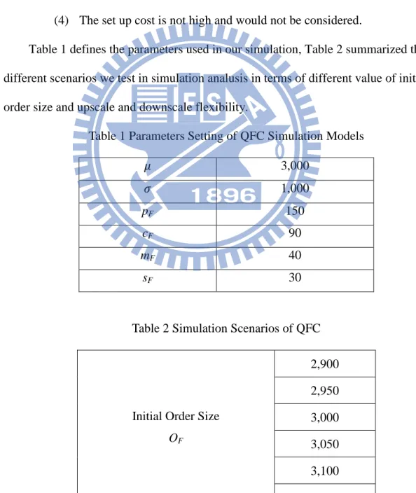
Table 1 defines the parameters used in our simulation, Table 2 summarized the different scenarios we test in simulation analusis in terms of different value of initial order size and upscale and downscale flexibility.
Table 1 Parameters Setting of QFC Simulation Models
3,000 1,000 pF 150 cF 90 mF 40 sF 30
Table 2 Simulation Scenarios of QFC
Initial Order Size OF 2,900 2,950 3,000 3,050 3,100 3,150
20 3,200 3,250 3,300 3,350 3,400 3,450 3,500
Upscale and Downscale Flexibility α = β 0 0.05 0.1 0.15 0.2
3.3 Simulation Modeling (Excel)
In our study, we use Microsoft Excel to design and implement our simulation analysis. Through this simulation model, we generate 500 samples to discuss the buyer’s profit, the supplier profit and total supply chain’s profit respectively to understand the effect of QFC.
Here we briefly summarize the simulation steps by using Excel.
Step 1: Set up the simulation parameters in the Excel spreadsheet based on Table 1. Step 2: Generating random numbers of market demand using Excel. We use the Excel function NORMINV (RAND (), μ, σ) to generate 1,000 samples of the random demand as defined in 2.4.1 that are normally distributed, with mean and standard deviation . Both μ and σ are based on the assumption of variables in section 3.2. Note that the first 500 sample points were not adopted to avoid the initial warm-up bias of the random number generator.
Step 3: Set up the formulas of supplier’s profit, buyer’s profit, total supply chain profit corresponding to the 500 samples of demand for each scenario based on the
21
formulas of section 3.1.
Step 4: Evaluate the average of the simulation results of 500 samples.
Step 5: Analysis for different scenarios. Using the Excel tool “Data Tables”, we generate different simulation results for different scenarios as shown in Table 2 and then use the Excel tool “Senario Manager” to generate different simulation results in terms of α and β described on Table 2.
(4a) Different OF for a given α and β.
(4b) For different values of α and β.
3.4 Simulation Results
From the simulation results, we have found that
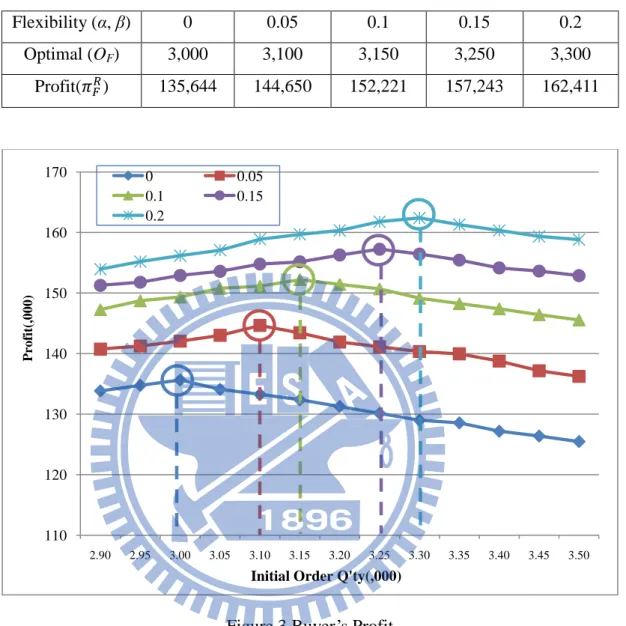
1. Table 3 indicates the optimal initial order quantity and corresponding profit of each given flexibilities for the buyer. Figure 3 shows the buyer’s profit under different flexibilities. Both the buyer’s initial order quantity and
corresponding profit increase while the flexibility (α and β) increases. The buyer gains around 12% from QFC in the case of α = β = 0.1. So that when the supply chain applies QFC and gives the buyer more flexibility on order quantities, the buyer would be willing to order more.
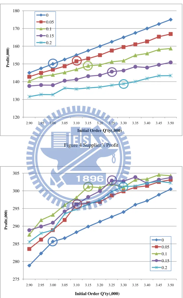
2. Figure 4 shows the supplier’s profit corresponding to the buyer’s initial order quantity under different flexibilities. The supplier’s profit goes down when the flexibility (α and β) increases except the reasonable flexibility. The supplier loses around 1% from QFC in the case of α = β = 0.1.
3. Figure 5 shows the total supply chain profit corresponding to the buyer’s initial order quantity under different flexibilities. From this Figure, we can find that QFC benefits the total supply chain. The total supply chain profit increases with the increased flexibility, except the flexibility is too large.
22
Table 3 Optimal OF for Different Flexibility (Buyer)
Flexibility (α, β) 0 0.05 0.1 0.15 0.2
Optimal (OF) 3,000 3,100 3,150 3,250 3,300
Profit( ) 135,644 144,650 152,221 157,243 162,411
Figure 3 Buyer’s Profit
110 120 130 140 150 160 170 2.90 2.95 3.00 3.05 3.10 3.15 3.20 3.25 3.30 3.35 3.40 3.45 3.50 Pro fit( ,0 0 0 )
Initial Order Q'ty(,000)
0 0.05
0.1 0.15
23
Figure 4 Supplier’s Profit
Figure 5 Total Supply Chain Profit
120 130 140 150 160 170 180 2.90 2.95 3.00 3.05 3.10 3.15 3.20 3.25 3.30 3.35 3.40 3.45 3.50 Pro fit( ,0 0 0 )
Initial Order Q'ty(,000)
0 0.05 0.1 0.15 0.2 275 280 285 290 295 300 305 2.90 2.95 3.00 3.05 3.10 3.15 3.20 3.25 3.30 3.35 3.40 3.45 3.50 Pro fit( ,0 0 0 )
Initial Order Q'ty(,000)
0 0.05 0.1 0.15 0.2
24
3.5 Sensitivity Analysis and Discussion
As mentioned above, we can find that QFC has a positive effect on the buyer, whereas the supplier suffers the loss from QFC. Once the supply chain apply the QFC, the more flexibility the supplier provides the more profit the supplier would lose. In the case of section 3.4, we know that buyer’s overstock cost is equal to the buyer’s
understock cost, Cu/Co=1, i.e. the product margin is equal to the leftover cost. What is the impact on the ordering quantity and the supply chain members if the product margin is higher or lower?
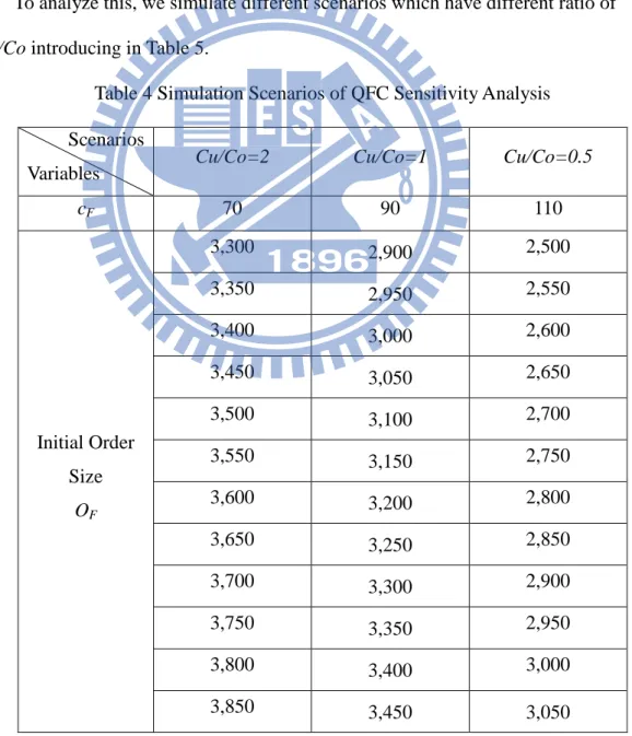
To analyze this, we simulate different scenarios which have different ratio of Cu/Co introducing in Table 5.
Table 4 Simulation Scenarios of QFC Sensitivity Analysis Scenarios
Variables Cu/Co=2 Cu/Co=1 Cu/Co=0.5
cF 70 90 110 Initial Order Size OF 3,300 2,900 2,500 3,350 2,950 2,550 3,400 3,000 2,600 3,450 3,050 2,650 3,500 3,100 2,700 3,550 3,150 2,750 3,600 3,200 2,800 3,650 3,250 2,850 3,700 3,300 2,900 3,750 3,350 2,950 3,800 3,400 3,000 3,850 3,450 3,050
25 3,900 3,500 3,100 Upscale and Downscale Flexibility α = β 0 0.05 0.1 0.15 0.2
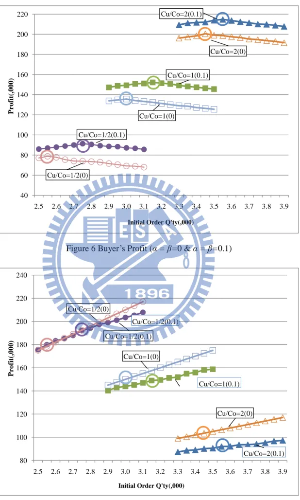
For simplifying, we only take α = β=0 and α = β=0.1as a example to introduce our finding as follows. The detailed simulation results are diagramed in Appendix A.
1. Figure 6 shows the buyer’s profit on various ratio of Cu/Co. It shows that the buyer always benefits from QFC. No matter the ratio of Cu/Co is high or low, both the buyer’s initial order quantity and profit increase with QFC. However, the buyer’s marginal profits are similar for different ratio of Cu/Co.
2. Figure 7 shows the supplier’s profit on various ratio of Cu/Co. If the ratio of Cu/Co is high, the supplier suffer loss more from QFC. However, if the ratio of Cu/Co is low, the supplier gain a little from QFC while the buyer orders less. In addition, the supplier loses less when the buyer orders less.
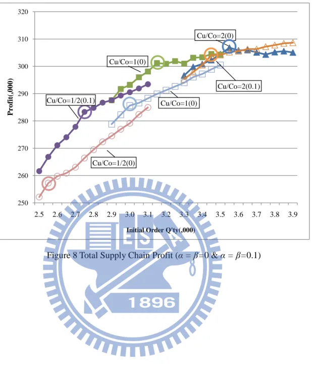
3. Figure 8 shows the total supply chain profit on various ratio of Cu/Co. It shows that the total supply chain always benefits from QFC. When the Cu/Co is higher, the marginal profit of the total supply chain is smaller.
4. Thus, QFC makes the supply chain much efficienctly. It favors the buyer and total supply chain but hurt the supplier. The higher the flexibility, the more benefit the buyer and total supply chain gain from QFC. In addition, the higher flexibility results in the higher initial order quantity.
26
Figure 6 Buyer’s Profit (α = β=0 & α = β=0.1)
Figure 7 Supplier’s Profit (α = β=0 & α = β=0.1)
40 60 80 100 120 140 160 180 200 220 2.5 2.6 2.7 2.8 2.9 3.0 3.1 3.2 3.3 3.4 3.5 3.6 3.7 3.8 3.9 P ro fit (, 0 0 0 )
Initial Order Q'ty(,000)
80 100 120 140 160 180 200 220 240 2.5 2.6 2.7 2.8 2.9 3.0 3.1 3.2 3.3 3.4 3.5 3.6 3.7 3.8 3.9 P ro fit (, 0 0 0 )
Initial Order Q'ty(,000)
Cu/Co=1/2(0.1) Cu/Co=1(0.1) Cu/Co=2(0.1) Cu/Co=1/2(0) Cu/Co=2(0) Cu/Co=1/2(0.1) Cu/Co=1(0) Cu/Co=1/2(0) Cu/Co=1/2(0.1) Cu/Co=1(0) Cu/Co=1(0.1) Cu/Co=2(0) Cu/Co=2(0.1)
27
Figure 8 Total Supply Chain Profit (α = β=0 & α = β=0.1)
250 260 270 280 290 300 310 320 2.5 2.6 2.7 2.8 2.9 3.0 3.1 3.2 3.3 3.4 3.5 3.6 3.7 3.8 3.9 P ro fit (, 0 0 0 )
Initial Order Q'ty(,000)
Cu/Co=1(0) Cu/Co=2(0) Cu/Co=1(0) Cu/Co=1/2(0) Cu/Co=1/2(0.1) Cu/Co=2(0.1)
28
IV. Analysis of Double-Ordering Contract
This chapter discusses the effect of DOC. In order to analyze the effect of the DOC, we contrast with the Single order contract (SOC). In this chapter, we first describe SOC in 4.1, and then describe DOC in 4.2. The following section 4.3 state our experimental design for both SOC and DOC. We then introduce the steps of our simulation models in 4.4. The section 4.5 indicates our simulation results. At the end of this chapter, we propose the sensitivity analysis of DOC simulation model and discuss the results in 4.6.
4.1 Single Order Contract Model Formulation
Single order contract(SOC) that the buyer only can order one time for the whole sales period before the sales season begins. Moreover, the buyer doesn’t allow changing its ordering quantity.
Here we consider a single supplier and a single buyer. The buyer placed a SOC order to the supplier.
We assume that the market demand of SOC is normal distributed, DX ~ N( , ),
with a mean of and standard deviation of .
To write more detailed SOC model formulation, we now define the following notations of SOC.
OX The buyer’s order quantity of Fixed contract
RX Realized demand quantity
Mean of quantity demanded
Standard deviation of quantity demanded SLX Service level
F-1 The inverse of the standard normal distribution oX The buyer’s overstock quantity
29
pX Selling price per unit
cX Wholesale price per unit.
mX Production cost per unit.
sX The buyer’s salvage value per unit. pX > cX > mX > sX > 0
Cost of overstocking by one unit, = cX - sX
Cost of understocking by one unit, = pX - cX
Supplier profit of Fixed contract Buyer profit of Fixed contract Total profit
The formulas of our SOC simulation model are described as follows. The buyer’s order quantity is
OX = F-1(SLX, , ) (10)
The buyer’s overstock quantity is
oX = max(0, OX – RX) (11)
The supplier profit is
= OX × (cX – mX) (12)
The buyer profit is
= min(DX, OX) × pX – OX × cX + oX × sX (13)
Total supply chai profit is
= + (14)
4.2 Double-Ordering Contract Model Formulation
Double-ordering contract (DOC) is widely used in fast fashion industry. For example, Benetton , used in the 1980, provides second order opportunity around the start of the season and can significantly reduce markdowns and leftover inventory.
30
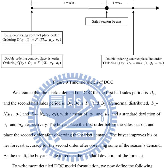
placed a DOC order to the supplier. Figure 9 introduces the timeline sketch of DOC.
Figure 9 Timeline sketch of DOC
We assume that the market demand of DOC for the first half sales period is , and the second half sales period is . Both and are normal distributed, ~ N( , ) and ~ N( , ), with a mean of and and a standard deviation of
and respectively. The buyer place the first order before the sales season, and place the second order afetr observing the market demand. The buyer improves his or her forecast accuracy for the second order after observing some of the season’s demand. As the result, the buyer is able to reduce the standard deviation of the forecast.
To write more detailed DOC model formulation, we now define the following notations of DOC.
Realized demand quantity of the first half sales period Realized demand quantity of the second half sales period SL Service level
F-1 The inverse of the standard normal distribution pD Selling price per unit
cD Wholesale price per unit.
Sales season begins
Double-ordering contract place 2nd order
Ordering Q’ty: = max (0, – )
6 weeks 1 week
Single-ordering contract place order Ordering Q’ty : OX = F-1(SLX, , )
Double-ordering contract place 1st order
31
mD Production cost per unit.
sD The buyer’s salvage value per unit. pD > cD > mD > sD > 0
Cost of overstocking by one unit, = cD - sD
Cost of understocking by one unit, = pD - cD
Supplier profit of the first sales period Supplier profit of the second sales period
Supplier profit of the entire sales period
Buyer profit of the first sales period Buyer profit of the second sales period
Buyer profit of the entire sales period Total profit
The formulas of our DOC simulation model are described as follows. The buyer’s first order quantity is
= F-1(SL, , ) (15)
The order-up-to level of the second half period is
= F-1(SL, , ) (16)
Buyer’s overstock quantity of first half period is
= max(0, – ) (17)
The buyer’s second order quantity is
= max(0, – ) (18)
Buyer’s overstock quantity of second half period is
= max(0, – ) (19)
Buyer’s understock quantity is
= max(0, – ) (20)
32
= × (cD – mD) (21)
Supplier profit of the second sales period is
= × (cD – mD) (22)
Supplier profit of the entire sales period is
= + (23)
Buyer profit of the first sales period is
= min ( , ) × pD – × cD (24)
Buyer profit of the second sales period is
= min ( , ) × pD – × cD – × sD (25)
Buyer profit of the entire sales period is
= + (26)
Total supply chain profit is
= + (27)
4.3 Experimental Design
In order to analyze the effect of DOC with the improved demand forecast, we experiment on scenarios which take account of the different standard deviation of the second order , which are given by different k fraction of . The smaller the k means the forecast is more accurate. And each scenario would simulate in terms of different SL.Besides, we assume that
(1) The supplier allows the buyer break up the purchase of the entire sales period into two orders. The first order covers the earlier half sales period, whereas the second order covers the latter half sales period. Thus,
= = (28)
=
33
(2) Since we assume the market information will improve the forecast, the standard deviation of quantity demanded of the second half sales period of DOC will be less than that of the first half sales period.
= k × , k 1 (30)
(3) In order to analyze the impact of DOC, we assume that the cost parameters of both SOC and DOC are the same.
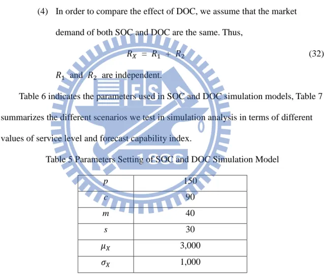
= , = , = , = (31) (4) In order to compare the effect of DOC, we assume that the market
demand of both SOC and DOC are the same. Thus,
= + (32)
and are independent.
Table 6 indicates the parameters used in SOC and DOC simulation models, Table 7 summarizes the different scenarios we test in simulation analysis in terms of different values of service level and forecast capability index.
Table 5 Parameters Setting of SOC and DOC Simulation Model
p 150 c 90 m 40 s 30 3,000 1,000
34 Service Level SL 0.25 0.3 0.35 0.40 0.45 0.50 0.55 0.60 0.65 0.70 0.75 0.80 0.85 0.90 0.95 Forecast Capability Index
k
1/3 1/4 1/5
4.4 Simulation Modeling (Excel)
In our study, we use Microsoft Excel to design and implement our simulation analysis. Through this simulation model, we generate 500 samples for both contracts to discuss the buyer’s profit, the supplier’s profit and total supply chain profit of each contract respectively to understand the effect of DOC.
Here we briefly summarize the simulation steps by using Excel.
Step 1: Set up the simulation parameters in the Excel spreadsheet based on Table IV-2.
Step 2: Generating random numbers of market demand using Excel. We use the Excel function NORMINV(RAND(), μ, σ) to generate 1,000 samples of the random demand as defined in 2.4.2. Both μ and σ are based on the assumption of variables in
35
section 4.3. Note that the first 500 sample points were not adopted to avoid the initial warm-up bias of the random number generator.
Step 3: Set up the formulas of supplier’s profit, buyer’s profit, total supply chain profit, buyer’s overstock and understock corresponding to the 500 samples of demand for each scenario based on the formulas in section 4.1 and 4.2.
Step 4: Evaluate the average of the simulation results of 500 samples.
Step 5: Analysis of different scenarios. Using the Excel tool “Data Tables”, we generate different simulation results in SL as shown in Table 7 and then we use the Excel tool “Scenario Manager” to generate different simulation results in terms of k described in Table 7.
(4a) Different SL for a given k. (4b) For different values of k.
4.5 Simulation Results
From the simulation results, we have found that
1. Figure 10 shows the buyer’s profit on SOC and DOC with various k. The buyer’s profit is increasing while the SL is higher. Under the same SL, the buyer’s profit with DOC is higher than that of SOC. The buyer’s profit with DOC is higher while k is smaller. Also, in this case, the optimal SL of DOC is larger than that of SOC. Furthermore, the margin of DOC profit and SOC profit increases with the increased SL.
2. Figure 11 shows the supplier’s profit on SOC and DOC with various k. The supplier suffers loss from DOC obviously. The margin of DOC loss and SOC loss increases with the increased SL. And it seems that the k doesn’t affect the profit.
36
The total supply chain profit is getting higher while the SL is higher. The total supply chain profit with DOC is better than that of SOC while SL is over 0.8. Furthermore, the impact from k decreases when SL is getting larger.
4. Thus, DOC favors the buyer and hurts the supplier. It makes total supply chain efficiently when SL is over 0.8. It seems that the better the buyer’s forecast capability doesn’t affect too much. Furthermore, applying DOC makes the buyer achieve higher SL and better satisfy customer’s needs.
Figure 10 Buyer’s Profit
80 90 100 110 120 130 140 150 160 170 0.25 0.30 0.35 0.40 0.45 0.50 0.55 0.60 0.65 0.70 0.75 0.80 0.85 0.90 0.95 P ro fit (, 0 0 0 ) Service Level SOC k=1/3 k=1/4 k=1/5
37
Figure 11 Supplier’s Profit
Figure 12 Total Supply Chain Profit
110 120 130 140 150 160 170 180 190 200 210 220 230 240 0.25 0.30 0.35 0.40 0.45 0.50 0.55 0.60 0.65 0.70 0.75 0.80 0.85 0.90 0.95 P ro fit (, 0 0 0 ) Service Level SOC k=1/3 k=1/4 k=1/5 240 250 260 270 280 290 300 310 320 330 0.25 0.30 0.35 0.40 0.45 0.50 0.55 0.60 0.65 0.70 0.75 0.80 0.85 0.90 0.95 P ro fit (, 0 0 0 ) Service Level SOC k=1/3 k=1/4 k=1/5
38
4.6 Sensitivity Analysis and Discussion
Same with QFC, as mentioned above, we can find that DOC has a positive effect on the buyer, whereas the supplier suffers a loss from DOC. In the case of section 4.5, we know that buyer’s overstock cost is equal to the buyer’s understock cost, Cu/Co=1, i.e. the product margin is equal to the leftover cost. What is the impact on the ordering quantity and the supply chain members if the product margin is higher or lower?
To analyze this, we simulate different scenarios which have different ratio of Cu/Co introducing in Table 8.
Table 7 Simulation Scenarios of DOC Sensitivity Analysis Scenarios
Variables Cu/Co=2 Cu/Co=1 Cu/Co=0.5
cF 70 90 110
For simplifying, we only take SOC and DOC with k = 1/4 as a example to introduce our finding as follows. The detailed simulation results are diagramed in Appendix B.
1. Figure 13 indicates the effect of DOC on the buyer’s profit under various ratio of Cu/Co. For the buyer, no matter the ratio of Cu/Co is higher or lower, the buyer benefits from DOC. However, the buyer benefits more when the ratio of Cu/Co is lower.
2. Figure 14 indicates the effect of DOC on the supplier’s profit under various ratio of Cu/Co. For the supplier, no matter the the ratio of Cu/Co is high or low, the supplier lose from DOC. In addition, the supplier loses more from DOC while the ratio of Cu/Co is smaller.
3. Figure 15 indicates the effect of DOC on total supply chain profit under various ratio of Cu/Co. It seems that the k doesn’t affect the total supply cahin
39
profit. And the total supply chain profit with DOC is better than that of SOC while SL is over 0.8. The profit increases approximate to 3% when SL is very high.
4. Thus, the DOC benefits the buyer, whereas the supplier suffers a loss from DOC. As to the total supply chain, DOC is effective only when the SL is high.
Figure 13 Effect of Buyer’s Profit (k=1/4)
-40 -20 0 20 40 60 80 100 120 140 160 180 200 220 240 0.25 0.3 0.35 0.4 0.45 0.5 0.55 0.6 0.65 0.7 0.75 0.8 0.85 0.9 0.95 P ro fit (, 0 0 0 ) Service Level Cu/Co=1/2(S) Cu/Co=1/2(D) Cu/Co=1(S) Cu/Co=1(D) Cu/Co=2(S) Cu/Co=2(D)
40
Figure 14 Effect of Supplier’s Profit (k=1/4)
Figure 15 Effect of Total Supply Chain Profit (k=1/4)
60 80 100 120 140 160 180 200 220 240 260 280 300 320 340 0.25 0.3 0.35 0.4 0.45 0.5 0.55 0.6 0.65 0.7 0.75 0.8 0.85 0.9 0.95 P ro fit (, 0 0 0 ) Service Level 240 250 260 270 280 290 300 310 320 330 0.25 0.3 0.35 0.4 0.45 0.5 0.55 0.6 0.65 0.7 0.75 0.8 0.85 0.9 0.95 P ro fit (, 0 0 0 ) Service Level Cu/Co=2(D) Cu/Co=1(D) Cu/Co=1/2(D) Cu/Co=2(S) Cu/Co=1(S) Cu/Co=1/2(S) Cu/Co=1/2(S) Cu/Co=1/2(D) Cu/Co=1(S) Cu/Co=2(S) Cu/Co=1(D) Cu/Co=2(D)
41
V. Conclusion
5.1 Research Summary
From the simulation experiments results, we can easily find that no matter QFC or DOC, the supply chain contracts benefit for the buyer undoubtedly. Whereas the
supplier suffers loss from QFC or DOC. As to the total supply chain, it benefits from supply chain contract under certain circumstances.
QFC always benefits the buyer, it not only improves the buyer’s profit and also gives the buyer incentive to order more quantity, especially when the supplier provides better flexibility. But the supplier suffer loss from it. However, it improves total supply chain profit, especially when the buyer’s product margin is relatively low. Thus, QFC probably is applied in the industry that the supplier’s production capacity is large. So that the supplier is willing to provide the flexibility to stimulate the buyer’s order and still can mainten his or her profit under a certain level.
As to DOC, it improves the supply chain efficiency only when service level is high. However, it always benefits the buyer but makes the supplier suffer loss. In addition, DOC request the QR system which the supplier needs to invest a lot to improve the manufacturing to meet fulfill the buyer’s needs promptly. This also should be
considered. So that rather than the decentralized system of supply chain, the DOC might be applied in the industry which is highly vertical integration or the centralized supply chain system, such as Zara and Benetton, in order to prompt response the market demand and market change effectively.
Smiling curve can be illustrated for this kind of phenomenon. Smiling curve had been proposed by Stan Shih, the founder of Acer. It is an illustration of value-added potentials of value chain in an IT-related manufacturing industry. According to Shih’s observation in PC industry both end of the value chain command higher value added to
42
the product than the middle part of the value chain. The following graph indicates the smiling curve phenomenon.
Figure 16 Smiling Curve
(Source: Wikipedia)
From this graph, we can realize the power structure in a supply chain. In this graph, the upstream and downstream channels own much power, whereas the middle members of the supply chain relatively weak. Corresponding to our analysis, while the supply chain members coordinate by the supply chain contract, the buyer might be more powerful resulting from the buyer always gains profit from these contracts.
Nevertheless, for the supply chain sustainability, the buyer cannot fully take the advantage. The buyer should also consider the incentive such as reward system or revenue sharing with the supplier while applying supply chain contracts.
5.2 Extension for Future Research
At the end of our study, we propose some aspects for future research.
1. In our study, we consider the unit cost vary stepwise with flexibility while the ordering quantity increase for QFC. For the DOC, it could be considered for future research that the unit cost of the second order can be higher than that of
43
the first order.
2. Our study is only discussing about a simple supply chain consisting of one buyer and one supplier, which produces and sells a single-period product. However, one supply chain always consists of several members in many echelons. The effect of aggregation could be considered for future discussion. 3. It’s also interesting to have an industrial survey to understand the application
of supply chain contract in industry.
4. As mentioned before, the supplier loses from the supply chain contract. Thus, the supplier reward system can be another interesting issue to consider.
44
Reference
1. Chopra, S. and P. Meindl, Supply chain management : strategy, planning, and operation. 3rd ed Upper Saddle River, N.J.: Pearson Prentice Hall. 2007. 2. Cachon, G., "Supply chain coordination with contracts". Handbooks in
operations research and management science, 2003. 11: p. 229-340. 3. Porter, M., Competitive advantage: Free Press New York. 1985.
4. Martin, C., Logistics and supply chain management: Financial Times, Prentice Hall. 1998.
5. Simchi-Levi, D., P. Kaminsky, and E. Simchi-Levi, Designing and managing the supply chain : concepts, strategies, and case studies. 3rd ed. Mcgraw-Hill/Irwin series operations and decision sciences Boston: McGraw-Hill/Irwin. 2008. 6. Stadtler, H., Supply chain management and advanced planning: concepts,
models, software, and case studies: Springer Verlag. 2008.
7. Harris, F., "How many parts to make at once". Operations Research, 1990. 38(6): p. 947-950.
8. Baker, K., "Safety stocks and component commonality". Journal of Operations Management, 1985. 6(1): p. 13-22.
9. Baker, K., M. Magazine, and H. Nuttle, "The effect of commonality on safety stock in a simple inventory model". Management Science, 1986. 32(8): p. 982-988.
10. Schneider, H. and J. Ringuest, "Power approximation for computing (s, S) policies using service level". Management Science, 1990. 36(7): p. 822-834. 11. Chen, F. and D. Krass, "Inventory models with minimal service level
constraints". European Journal of Operational Research, 2001. 134(1): p. 120-140.
12. Bollapragada, R., U. Rao, and J. Zhang, "Managing inventory and supply performance in assembly systems with random supply capacity and demand".
45
Management Science, 2004. 50(12): p. 1729-1743.
13. Tsay, A., S. Nahmias, and N. Agrawal, "Modeling supply chain contracts: A review". Quantitative models for supply chain management, 1999. 17: p. 299¡V336.
14. Tsay, A.A., "The quantity flexibility contract and supplier-customer incentives". Management Science, 1999. 45(10): p. 1339-1358.
15. Eppen, G.D. and A.V. Iyer, "Backup agreements in fashion buying - The value of upstream flexibility". Management Science, 1997. 43(11): p. 1469-1484. 16. Tsay, A.A. and W.S. Lovejoy, "Quantity flexibility contracts and supply chain
performance". Manufacturing & Service Operations Management|Manufacturing & Service Operations Management, 1999. 1(2): p. 89-111.
17. Barnes-Schuster, D., Y. Bassok, and R. Anupindi, "Coordination and flexibility in supply contracts with options". Manufacturing & Service Operations
Management, 2002. 4(3): p. 171-207.
18. Fisher, M. and A. Raman, "Reducing the cost of demand uncertainty through accurate response to early sales". Operations Research, 1996. 44(1): p. 87-99. 19. Iyer, A.V. and M.E. Bergen, "Quick response in manufacturer-retailer channels".
Management Science, 1997. 43(4): p. 559-570.
20. Lau, H.S. and A.H.L. Lau, "Reordering strategies for a newsboy-type product". European Journal of Operational Research, 1997. 103(3): p. 557-572.
21. Lau, A.H.L. and H.S. Lau, "Decision models for single-period products with two ordering opportunities". International Journal of Production Economics, 1998. 55(1): p. 57-70.
22. Choi, T.M., D. Li, and H. Yan, "Optimal two-stage ordering policy with Bayesian information updating". Journal of the Operational Research Society, 2003. 54(8): p. 846-859.
46
Appendix A QFC Simulation Results
Figure A-1 Buyer’s Profit (Cu/Co=2)
Figure A-2 Supplier’s Profit (Cu/Co=2)
185 190 195 200 205 210 215 220 225 230 3.30 3.35 3.40 3.45 3.50 3.55 3.60 3.65 3.70 3.75 3.80 3.85 3.90 Pro fit( ,0 0 0 )
Initial Order Q'ty(,000)
0 0.05 0.1 0.15 0.2 70 75 80 85 90 95 100 105 110 115 120 3.30 3.35 3.40 3.45 3.50 3.55 3.60 3.65 3.70 3.75 3.80 3.85 3.90 P ro fit (, 0 0 0 )
Initial Order Q'ty(,000)
0 0.05
0.1 0.15
47
Figure A-3 Total Supply Chain Profit (Cu/Co=2)
Figure A-4 Buyer’s Profit (Cu/Co=1/2)
290 294 298 302 306 310 314 3.30 3.35 3.40 3.45 3.50 3.55 3.60 3.65 3.70 3.75 3.80 3.85 3.90 P ro fit (, 0 0 0 )
Initial Order Q'ty(,000)
0 0.05 0.1 0.15 0.2 60 65 70 75 80 85 90 95 100 105 2.50 2.55 2.60 2.65 2.70 2.75 2.80 2.85 2.90 2.95 3.00 3.05 3.10 Pro fit( ,0 0 0 )
Initial Order Q'ty(,000)
0 0.05
0.1 0.15
48
Figure A-5 Supplier’s Profit (Cu/Co=1/2)
Figure A-6 Total Supply Chain Profit (Cu/Co=1/2)
170 175 180 185 190 195 200 205 210 215 220 2.50 2.55 2.60 2.65 2.70 2.75 2.80 2.85 2.90 2.95 3.00 3.05 3.10 P ro fit (, 0 0 0 )
Initial Order Q'ty(,000)
0 0.05 0.1 0.15 0.2 250 255 260 265 270 275 280 285 290 295 300 2.50 2.55 2.60 2.65 2.70 2.75 2.80 2.85 2.90 2.95 3.00 3.05 3.10 P ro fit (, 0 0 0 )
Initial Order Q'ty(,000)
0 0.05 0.1 0.15 0.2
49
Appendix B DOC Simulation Results
Figure B-1 Buyer’s Profit (Cu/Co=2)
Figure B-2 Supplier’s Profit (Cu/Co=2)
170 180 190 200 210 220 230 0.25 0.30 0.35 0.40 0.45 0.50 0.55 0.60 0.65 0.70 0.75 0.80 0.85 0.90 0.95 P ro fit (, 0 0 0 ) Service Level SOC k=1/3 k=1/4 k=1/5 60 70 80 90 100 110 120 130 140 150 0.25 0.30 0.35 0.40 0.45 0.50 0.55 0.60 0.65 0.70 0.75 0.80 0.85 0.90 0.95 P ro fit (, 0 0 0 ) Service Level SOC k=1/3 k=1/4 k=1/5