回歸平均的探索

全文

(1)國立交通大學財務金融研究所碩士論文. 回歸平均的探索 An Exploration for Mean Reversion. 研究生：陳君婷指導教授：李昭勝博士鍾惠民博士. 中華民國九十六年六月.

(2) 回歸平均的探索 An Exploration for Mean Reversion. 研究生：陳君婷. Student : Chun-Ting Chen. 指導教授：李昭勝博士. Advisor : Dr. Chao-Sheng Lee. 鍾惠民. 博士. Advisor : Dr. Hui-Min Chung. 國立交通大學財務金融研究所碩士班碩士論文. A Thesis Submitted to Graduate Institute of Finance National Chiao Tung University in partial Fulfillment of the Requirements for the Degree of Master of Science in Finance June 2007 Hsinchu, Taiwan, Republic of China. 中華民國九十六年六月.

(3) 回歸平均的探索. 研究生 : 陳君婷. 指導教授:李昭勝博士鍾惠民博士. 國立交通大學財務金融研究所碩士班 2007 2007 年 6 月. 摘要. 回歸平均在金融市場以很多不同的形式存在，且這些形式都符合於有效率的市場。然而，投資者與學者意味的回歸平均定義始終缺乏。本文提出關於時間序列回歸平均的定義且領悟平均隨時間變化的潛在意義。使用波動率指數、美國十年公債的利率與布蘭特原油和西德州中級原油的價差之周資料，估計回歸平均的水平與速度。結果顯示回歸平均的現象並非永續而是間斷性地存在，且不同的時間週期導致不一致的結果。. 關鍵字：自我相關、卡方檢定、指數權重移動平均法、幾何布朗運動、最大概似估計法、回歸平均、OU 隨機過程、定態隨機過程。. i.

(4) An Exploration for Mean Reversion. Student: Chun-Ting Chen. Advisor: Dr. Chao-Sheng Lee Advisor: Dr. Hui-Min Chung. Graduate Institute of Finance National Chiao Tung University June 2007. ABSTRACT Mean reversion exists in many different forms within financial markets, and none of these forms is necessarily inconsistent with efficient markets. However, there is a lack of precision in what many investment practitioners and scholars mean by the term “mean reversion”. In this paper, we propose a formal definition of what most investment practitioners and scholars seem to mean by “mean reversion”. In this paper, we recognize the potential significance of time variation in price reversion, and propose a time-dependent definition of mean reversion, which is based on the Ornstein-Uhlenbeck (O-U) process and the Geometric Brownian Motion (GBM). Using weekly data of VIX (Volatility Index) traded in CBOE from 1990 to 2007, interest rate of the United States Treasury Benchmark Bond 10-year from 1984 to 2007 and the spread between Brent crude oil and West Texas Intermediate crude oil traded in NYMEX from 1997 to 2007 to estimate the level and speed of mean reversion, and we show that the mean reversion phenomenon is not persistent but recurring, and there are inconsistent results by using different time scales.. Keywords: Autocorrelation, Chi-Square test, EWMA, GBM, Maximum Likelihood Estimation, Mean reversion, O-U process, Stationary.. ii.

(5) 誌謝. 首先誠摯的感謝指導教授李昭勝博士及鍾惠民博士，兩位老師悉心的教導使我得以探索回歸平均(Mean Reversion)領域的深奧，不時的討論並指點我正確的方向，使我在這些年中獲益匪淺。雖然李昭勝老師的逝去是我研究生涯中的遺憾，但老師對於學問的嚴謹是晚輩學習的典範。本論文的完成尤其要感謝牛維方學長的大力協助，不厭其煩的指出我研究中的缺失，且總能在我迷惘時為我解惑，使得本論文能夠更完整而嚴謹，你對於我的幫忙我銘記在心。另外亦得感謝中興大學應用數學系的林宗儀教授，台中技術學院風險管理與保險系的林淑惠教授、交通大學資訊與財金管理學系的周幼珍教授三位口試委員，因為有您們的建議及幫忙，使得本論文能夠更完整而嚴謹。也感謝同學的熱情幫忙與包容，恭喜我們順利走過這兩年。兩年裡的日子，研究室裡共同的生活點滴，學術上的討論、言不及義的閒扯、讓人又愛又怕的宵夜、趕作業的革命情感，感謝眾位學長姐、同學、學弟妹的共同砥礪，你/妳們的陪伴讓兩年的研究生活變得絢麗多彩。家人在背後的默默支持更是我前進的動力，你們的體諒、包容，讓我可以專心致力在課業上。有你們的支持與鼓勵，相信未來的生活將是很不一樣的光景。最後，謹以此文獻給我摯愛的雙親與李昭勝老師。願老師以我為榮!. iii.

(6) CONTENTS. Chinese Abstract ...........................................................................................................i English Abstract ...........................................................................................................ii Chinese Acknowledgements .......................................................................................iii Contents .......................................................................................................................iv List of Figures...............................................................................................................v I. II.. Introduction..........................................................................................................1 Definitions and Models....................................................................................2 2.1 Commonly Used Definitions.......................................................................2 2.2 Models Regarding Mean Reversion ..........................................................6. III.. Desired Properties of Mean Reversion...........................................................7. IV.. Statistical Inference for Mean Reversion of a Time Series ..........................8 4.1 Estimating the Level of Mean Reversion ..................................................9 4.2 Hypothesis Testing about Mean Reversion.............................................14. V.. Conclusions.........................................................................................................22. Reference ....................................................................................................................23 Appendix.....................................................................................................................26. iv.

(7) List of Figures. Figure 1.. Estimator for Level of Mean Reversion……………………….…...13. Figure 2.. MLE for Speed of Mean Reversion…………………………….…..16. Figure 3.. Chi-Square Test for Volatility Index……………………………….19. Figure 4.. Chi-Square Test for Interest Rate of U.S. Treasury Bond 10-Year……………………………...……………………………….20. Figure 5.. Chi-Square Test for Spread of Crude Oil between Brent and WTI………………………………………………..………..……….21. v.

(8) Introduction. I.. The theoretical significance of mean reversion of asset prices or returns in financial markets has long been recognized as crucial in discussions of predictive ability, arbitrage, hedging behavior, and derivative valuation. Many authors have examined the presence of mean reversion for the price spread between spot and future under arbitrage free condition. Negative correlation between the futures risk premium and spot prices is generally assumed. Many studies have also shown that the processes of financial asset prices can be characterized as mean-reverting. For example, Bessembinder, Coughenour, Seguin, and Smoller (1995) investigated serial correlations in agricultural, financial, and precious metal prices. MacKinlay and Ramaswamy (1988) found the mean reversion existed in the changes of the stock index futures basis. Significant mean-reverting behaviors are also found by Fama and French (1988b), who examine first-order autocorrelation coefficients of long-horizon real stock returns. More evidence can also be found in Lo and MacKinlay (1988); Poterba and Summers (1988); and Bonomo and Garcia (1994). Mean reversion is generally cited as a property of a stochastic process that tends to revert back to some normal level over long time when it is away from the level. This normal level is often called the mean or trend of the variable underlying the stochastic process. However, there is indeed lack of precision in what the “mean reversion” is. Furthermore, empirical investigations concerning mean reversion to date almost focus on static examinations. Actually, mean reversion of a process might be time-dependent with different scales. In fact, Ahmet, Norman, and Tian (2001) recognize the potential significance of time variation in price reversion, and propose a time-dependent definition of mean reversion, which is based on the term-structure of prices. Generally, many mean-reverting behaviors are measured over long horizons or infinite time. But investment practitioners are often interested in how the prices change over short time horizons, not long horizons. And they are also interested in the 1.

(9) speed of mean reversion. A serious obstacle in detecting mean reversion is the absence of reliable long time series, especially because mean reversion, if it exists, is thought to be slow and can only picked up over long horizons. For example, Fama and French (1988a), and Poterba and Summers (1988) provide direct empirical evidence that mean reversion occurs in U.S. stock prices over long horizons. But Lo and MacKinlay (1988) find evidence against mean reversion in U.S. stock prices using weekly data. Richardson (1989) also shows that by ignoring the interdependence among measures of mean reversion at different time horizons, interpretations that focus on individual horizon statistics can be misleading. Thus, we will give a new definition of mean reversion, and infer the desired properties of mean reversion with different time scales. This paper is organized as follows. In Section II, we first review commonly used definitions for mean reversion. As we shall see, there is no existing universal measure of “mean reversion” and the definition that we believe investment professionals often struggle towards is not like some other standard definition of time series analysis (namely “stationary”). In Section III, three examples are used to illustrate if these definitions are compliant with the common intuition about mean reversion. In Section IV, from a statistical view of point, we try to propose a definition for mean reversion and illustrate how it works. Concluding remarks and extensions for future researches are presented in Section V.. II.. Definitions and Models. 2.1 Commonly Used Definitions As discussed in the introduction, there are many possible definitions of mean reversion, which seems to mean different things to different people. Scholars discuss mean reversion by assuming that prices return to a fixed level or a trend path over infinite time. The most common definition is probably as follows:. 2.

(10) Definition 1: An asset model is mean reverting if the prices tend to some constant in long-horizon time given information available now.. Many scholars used this property of mean reversion to propose more stochastic models. For example, the GARCH model proposed by Bollerslev (1986) also assumed that there is a long-term average variance rate. Using this definition, many analysts can convince themselves that volatilities obviously mean revert without violating the trivial market efficient and arbitrage free conditions. The problem with this definition is that the level of mean reversion may be time-varying. There can be found enormous number of examples for which a trend can be viewed as the target of mean reversion, for instance, the nondurable goods index discussed in Ramsay and Silverman (2002). Under finite time horizon and discrete observations, autocorrelation of prices or returns is a well-known attribute commonly referred to as “mean reverting”. This gives the second definition of mean reversion:. Definition 2: An asset model is mean reverting if the returns or prices are negatively auto-correlated.. The general autoregressive process of order p in discrete time can be expressed as follows: Rt = µ + φ1 Rt −1 + φ 2 Rt − 2 + L + φ p Rt − p + ε t. (1). where φi ’s are autocorrelation coefficients on the i-th lagged term and ε t ’s are standard normal innovations. However, with different values of φi ’s, the process (1) does not necessarily converge. This means that a process can be negatively auto-correlated but diverges in long-horizon time, and so Definition 2 may be contrary to Definition 1. Therefore, the first-order autoregressive process AR(1) is popularly used in financial markets or academic researches.. 3.

(11) Then there comes to the sort of process discussed in Lee (1991): “Under this model, which has wide intuitive appeal, a below average price in one period is likely to be followed by “compensatory” above average prices in subsequent periods.” Rt = µ + φ (µ − Rt −1 ) + σε t. (2). where Rt is the return price in period t , µ is the unconditional mean return in a single period, ε t ’s are standard normal innovations, σ is volatility, and φ is positive coefficient that also means the negative autocorrelation coefficient. The middle term on the right-hand side, the mean reversion term, measures the deviation of this process from the mean in the previous period and adds the correction with weight φ . If the process was below the mean in the previous period, the process gets a. φ -kick upward; if it was above the mean, downward. That is, equation (2) captures a concept of mean reversion that explicitly models negative autocorrelations. It has frequently been said for example that the fantastic returns achieved in the 1980s were really a catching up exercise to make up for the poor returns in the 1970s. Jegadeesh (1991) also found the evidence that the monthly returns on the equally weighted index of stocks traded on the NYSE exhibits mean reversion over the period 1926-1988, according as the series of returns is found to exhibits significant negative serial correlation. In order to assess the informal evidence for this form of mean reversion in equity markets, Exley, Mehta, and Smith (2004) looked at 100 years of equity return data in 16 countries (the decennial Dimson, Marsh, and Staunton (2003) data set, split according to returns in each decade of the last century) and found no evidence that poor (good) returns in one decade are followed by good (poor) returns in the next. However, when the authors looked at the UK annual equity return data, they found that returns in a year are negatively correlated (-0.2) in the data set with returns in the subsequent two years. Lee’s definition refers to the 1980s “catching up” with the 1970s, so the returns in these decades were negatively auto-correlated if we looked at discrete decades. But presumably if we had just looked at annual periods we would 4.

(12) have found that the returns in the 1980s were generally above average and all returns in the 1970s generally below average. This would seem to maybe suggest an element of positive autocorrelation if we change the time scales. So it seems that there is also some uncertainty as to whether mean reversion is a positive or negative autocorrelated phenomenon. Equation (2) for the asset price process is in fact an example of a called stationary process. It is sometimes confusing about the difference between stationary process and mean reversion. In fact, stationary indeed provides another view to the concept of mean reversion.. Definition 3: An asset model is mean reverting if growth rates or volatilities are stationary.. A stationary process has identical distributions over time, unconditional on the immediate past. Under suitable conditions, the sample distribution of observations over a very long time period will converge to the stationary distribution. If an observation falls high up in the tail of the stationary distribution, it is likely that the following observation will be nearer to the long term average. This can give the appearance of a force driving observations over time towards a long term mean. This mean reverting force is countered by the influence of random noise which pushes the process away from its current value. Stationary series have proved fruitful for analyzing economic quantities such as interest rate, or dividend yields because at first sight it is plausible that these have a natural long term mean level. Exley, Mehta, and Smith (2004) mentioned that there exists mean reversion phenomenon in equity risk premium by using a stationary drift (or growth rate) process. They found that the evidence for mean reversion in equity market return volatility is also strong by using the data for 3-month and 5-year implied volatilities on the FTSE 100 (approximately the last 10 years) and DJ Euro-Stoxx Indices (approximately the last 5 years). However the corresponding asset prices can already reflect either deterministic or 5.

(13) stochastic mean reversion in volatility so that we do not observe any associated mean reversion in prices. Asset prices may continue to describe a random walk despite the stationary of these associated processes. Another problem with this definition is that a stationary process has the same distribution at every point in time which means that the mean price is the same over all time period. But we discussed the various functions of the mean reversion at different time scales in the introduction. And it might be allowed that the mean reversion is simple dependent. Before proposing our definition of mean reversion, we first discuss the implication of above three definitions. The Definition 1 does not imply the other two definitions because the long-term mean can not imply the negative auto-correlated and stationary processes. But the Definition 3 implies the Definition 1 because the prices are reverting to a stationary variable under the Definition 3, which means that the expectations are the same at any time and exist a long-term mean. And the Definition 2 also implies the Definition 1 because if the process value was below the mean in the previous period, the process gets an upward; if it was above the mean, downward. This means that the process exist a long-term constant mean. However, we can not find out any implications between Definition 2 and 3. These three definitions are popularly used in finance about mean reverting, but they may be inconsistent whether the asset prices are mean reverting.. 2.2 Models Regarding Mean Reversion Interest rates and volatilities of returns of assets are the quantities that are most frequently referred as mean reverting in finance. Traditionally there are models dedicated to describe them. The Ornstein-Uhlenbeck (O-U) process is a well-known stochastic process with an analytic solution of mean reversion. Vasicek (1977) uses it for describing the evolution of interest rates. The model specifies that the instantaneous interest rate follows the stochastic differential equation: dX t = κ (µ − X t )dt + σdWt 6. (3).

(14) In equation (3), µ and κ are respectively the level and speed of mean reversion. Hull and White (1990) extended (3) with both µ and κ to be time dependent. Another extension is the CIR (Cox, Ingersoll, and Ross, 1985) model that is also commonly used in describing interest rate. In a stochastic differential equation form, the model can be expressed as dX t = κ (µ − X t )dt + σ X t dWt. (4). As the model yields the non-central χ 2 distribution as its solution, each points of the process can be guaranteed to be positive almost surely. A broader class of models is the CEV (Constant Elasticity of Variance) model proposed by Cox and Ross (1976) which can be expressed as dX t = κ (µ − X t )dt + σX tβ / 2 dWt. (5). Similar to the CIR model, all values of the process are positive almost surely. Besides for modeling interest rates, these models are also used for volatilities, for example Heston (1993). It is noted that all of these models describe mean reversion at a very short time horizon with the term κ (µ − X t )dt . This illustrate the very basic idea that the level of the process will always tend to be lower if it is higher than its level of mean reversion, and tend to higher if it is lower than its level of mean reversion.. III.. Desired Properties of Mean Reversion. In this section, we illustrate the desired properties of mean reversion by investigating three processes, the Ornstein-Uhlenbeck (O-U) process, Brownian motion and simple harmonic motion (SHM). The O-U process is widely utilized in financial modeling, especially for interest rate. For example, Vasicek (1977) pioneered the application of such mean reverting stochastic processes for interest rate modeling. In fact, the O-U process can be viewed as a typical mean-reverting process since at every moment the process tends to move toward the level of mean reversion. Clearly the O-U process satisfies Definitions 1-3. For model (3), it is seen that the 7.

(15) long-term mean converges to µ, that is lim Et (X T Ω t ) = µ . As the process indeed T →∞. arises from an AR(1) process, it is easy to derive that two consecutive segments X t − X t −1 and X t −1 − X t −2 are negatively correlated with coefficient of correlation 1 − e −κt . Furthermore, as t → ∞ , the distribution converges to a normal distribution with mean µ and variance σ 2 2κ . The Brownian motion has totally different properties. As it diverges for very long horizon, neither the limit distribution nor the long-term mean exist. Consecutive segments are independent instead negatively correlated. Thus the Brownian motion can be viewed as a stereotype of processes that are not mean-reverting. Comparing with the O-U process and the Brownian motion, it is a little confusing that the simple harmonic motion (SHM) is mean reverting or not. Unlike the two counterparts, the SHM does not satisfy the above definitions, but it is always mean reverting to the mean level with a fixed frequency. Intuitively the SHM, say xt = sin t , passes the zero (or any points between -1 and 1) infinitely often and thus there’s no doubt that SHM is mean-reverting. However, the SHM does not converge to any constant nor has an obvious asymptote. The serial dependence also counts on the sampling frequency. For example, as the samples are taken from the region (0, π 2) with very high frequency, the path rises persistently, so the coefficient of correlation must be positive. It is readily seen that the Definitions 1 and 2 are not satisfied. To sum up, both the O-U process and the Brownian motion can be clearly shown to be mean reverting or not, but the simple harmonic motion may be suspicious. Indeed, it seems hard to provide a rigorous definition to identify the mean reversion properties of all processes. However, it seems possible and worth to investigate the mean reversion properties of discretely observed time series by extending Definition 2.. IV.. Statistical Inference for Mean Reversion of a Time Series. Among most of the above definitions and the commonly used models, the concept of mean reversion involves about the instantaneous behavior of the process or some 8.

(16) characteristics at an infinitely long time. However, in practical applications data are generally discretely observed and so only Definition 2 is feasible here. By extending Definition 2, we propose the following definition for the mean reversion of a time series.. Definition 4: A time series X t , t = 1,2,3, L , is mean reverting if there exists a function. µ t ≡ µ (t , X 0 , L, X t ). such. that. E t ( X t +1 | Ω t ). xt < µ t and in (µ t , xt ) if xt > µ t . The quantity κ t = − log. lies. in. (xt , µ t ). if. E ( X t +1 ) − µ t is the speed X t − µt. of mean reversion at time t.. It is easy to see that the definition is compliant with the concept of mean reversion by the stochastic differential equations. Also an AR(1) process with a negative coefficient of correlation satisfies this definition. But processes satisfying this definition do not necessarily converge in distribution or have a mean for long time. By this definition, level and speed of mean reversion are in a sense confounding. That is, each target of mean reversion µ t corresponds to a different speed of mean reversion κ t . But such characteristics enable dealing with non-stationary processes. On analyzing time series with this approach, a class of µ t can be taken into consideration as the candidates of the target of mean reversion, for example an EWMA (Exponentially Weighted Moving Average) predictor or some other nonlinear functions of observations.. 4.1 Estimating the Level of Mean Reversion Next, we discuss how the historical data can be used to estimate of the levels of mean reversion. In many instances, authors assume that the mean is constant over all time period. As a consequence, in the forecast computations each observation carries the same weight. However, the assumption of a time invariant is restrictive, and it would be more reasonable to allow for a mean that moves slowly over time. 9.

(17) Heuristically, in such a case it would be reasonable to give more weight to the most recent observations and less to the observations in the distant past. The exponentially weighted moving average (EWMA) model is a particular case of the model where the weights decrease exponentially as we move back through time. In this paper, we will use the O-U stochastic process as mean reverting model. Using weekly data of VIX (Volatility Index) traded in CBOE from 1990 to 2007, interest rate of the United States Treasury Benchmark Bond 10-year from 1984 to 2007, and spread between Brent crude oil and West Texas Intermediate (WTI) crude oil traded in NYMEX from 1997 to 2007 to investigate the phenomenon of mean reversion with different time scales. Continuous time models are useful for the theoretical properties, but in reality the trajectories of the process cannot be observed continuously, and the process must be sampled in discrete time. For estimation and testing purposes, a discrete time analogue of the continuous time model is required. First, we consider the locally constant mean model: X n+ j = µ + ε n+ j where µ is a constant mean level and ε n+ j is a sequence of uncorrelated errors. If one chooses weights that decrease geometrically with the age of the observations, the forecast of the future observation at time n can be calculated from. µˆ n = (1 − ω )X n + ωµˆ n−1. (6). where X t is the asset price, µˆ n is the estimate of the mean price for time n , and the weight ω is a constant between zero and one. Equation (6) shows how the forecast can be updated after a new observation has become available and expresses the new forecast as a combination of the old forecast and the most recent observation. The coefficient ω depends on how fast the mean level changes. If ω is small, more weight is given to the last observation and the information from previous periods is heavily discounted. If ω is close to 1, a new observation will change the old forecast only very little. Through repeated application of Equation (6), we can see that µˆ n is an 10.

(18) exponentially weighted average of previous observations, which can be shown that n −1. µˆ n = (1 − ω )∑ ω t X n −t + ω n µˆ 0. (7). t =0. Thus the influence of µˆ 0 on µ n is negligible, provided n is moderately large and. ω is smaller than 1. We take the available historical data X 1 as the initial estimate of µˆ 0 . Second, we consider the locally linear trend mean model: X n + t = µ + β t + ε n +t where µ is the intercept and β is the slope of the linear trend mean. Ordinary least squares leads to the following estimates at time 0: N. βˆ0 =. . ∑  t − t =1. N + 1 X t 2 .  N +1 t −  ∑ 2  t =1  N +1 µˆ 0 = X − βˆ0 2 N. 2. N  N + 1 12∑  t − X t 2  t =1  = N3 − N. (8). where N denotes the number of observations. We follow an approach originally used by Holt (1957) to introduce the updating equations. We assume a linear trend for the mean µ t and write it in slightly different form µ t = µ n + (t − n )β . Then the mean at time n + 1 is be defined as µ n +1 = µ n + β . An estimate of this mean can be found from two different sources: (1) from X n+1 , which represents the present estimator of. µ n+1 , and (2) from µˆ n + βˆ n , which is the estimator of µ n+1 from observations up to and including time n . Note that βˆ n is the estimate of the slope at time n . Holt considers a linear combination of these estimates,. (. µˆ n +1 = (1 − ω1 ) X n +1 + ω1 µˆ n + βˆ n. ). where α 1 = 1 − ω1 is a smoothing constant that determines how quickly past information is discounted. Similarly, information about slope comes from two sources: (1) from the difference of the mean estimators µˆ n +1 − µˆ n , and (2) from the previous estimator of the slope βˆ n . Again these estimates are linearly weighted to give 11.

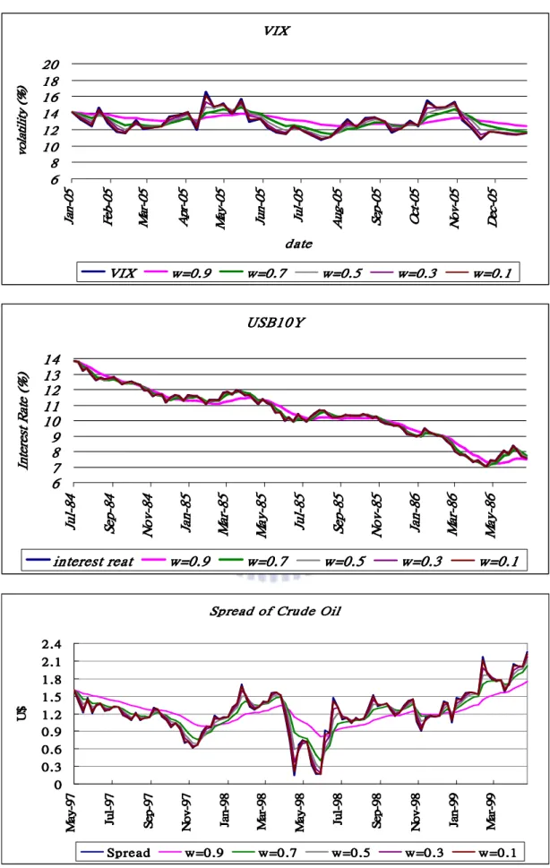
(19) βˆ n +1 = (1 − ω 2 )(µˆ n+1 − µˆ n ) + ω 2 βˆ n Thus, the parameter estimates are updated according to. (. µˆ n +1 = (1 − ω1 ) X n +1 + ω1 µˆ n + βˆ n. ). βˆ n +1 = (1 − ω 2 )(µˆ n +1 − µˆ n ) + ω 2 βˆ n. (9). We define the two different smoothing coefficients as ω1 = ω 2 and ω 2 = 2ω (1 + ω ) where the coefficient ω depends on how fast the mean level changes. Figure 1 shows how fast the mean level changes by using the weekly data of VIX, interest rate of the United States Treasury Benchmark Bond 10-year, and spread between Brent crude oil and West Texas Intermediate crude oil traded in NYMEX. If. ω is small, more weight is given to the last observation and the mean level is closer to the new observation. On the other way, if ω is close to 1, a new observation will change the old forecast only very little and the mean level changes smoothly. Figure 1 also shows that the locally constant mean model would be appropriate method for the data of VIX and spread of crude oil, and the locally downward linear trend mean would be appropriate method for the data of the United States Treasury Benchmark Bond 10-year.. 12.

(20) VIX 20 18 ) (% 16 y ti 14 li t 12 la o 10 v 8 6. 5 -0 n a J. 5 -0 b e F. 5 -0 r a M. VIX. 5 -0 y a M. 5 -0 r p A. w=0.9. 5 -0 n u J. 5 -0 g u A. 5 -0 l u J. date w=0.7 w=0.5. 5 -0 p e S. 5 -0 t c O. 5 -0 v o N. w=0.3. 5 -0 c e D. w=0.1. USB10Y ) % ( e t a R ts e r e t n I. 14 13 12 11 10 9 8 7 6. 4 8 -l u J. 4 8 p e S. 4 8 v o N. interest reat. 5 8 n a J. 5 8 -r a M. w=0.9. 5 8 y a M. 5 8 -l u J. w=0.7. 5 8 p e S. 5 8 v o N. w=0.5. 6 8 n a J. 6 8 -r a M. w=0.3. 6 8 y a M. w=0.1. Spread of Crude Oil. $U. 2.4 2.1 1.8 1.5 1.2 0.9 0.6 0.3 0. 79ya M. 79luJ Spread. 79peS. 79vo N w=0.9. 89naJ. 89ra M w=0.7. 89ya M. 89luJ w=0.5. 89peS. 89vo N w=0.3. 99naJ. 99ra M w=0.1. Figure 1. Estimator for Level of Mean Reversion: Index series and mean level series with different weight of the VIX (top) and interest rate of the United States Treasury Benchmark Bond 10-year 13.

(21) (middle), and spread between Brent crude oil and West Texas Intermediate crude oil traded in NYMEX (bottom). The fact is that the mean level changes faster with. ω = 0.9. ω = 0.1. than ω. = 0.9 . The weight. is better choice because we expect the mean level series changes smoothly which is. suggested by Brown (1962).. 4.2 Hypothesis Testing about Mean Reversion According to EWMA model with locally constant mean, we can calculate the estimate of the mean price for time n ( µˆ n ) by historical data ( X 1 , X 2 , L , X n ), and l-step-ahead forecast of mean from time original n by µˆ n +l = µˆ n . The forecasts are the same for all l. Therefore, the distribution of the price X t which follows the O-U process with constant mean is.  σ2 X t ~ N  µˆ n + e −κ ( X t −1 − µˆ n ), 1 − e − 2κ 2κ . (. ) . and the log likelihood function is given by. [. ]. n ( X t − µˆ n ) − e −κ ( X t −1 − µˆ n ) n 2 log L = constant − log τ − ∑ 2 2τ 2 t =1. ( ). c. 2. (10). σ2 ( 1 − 2e −κ ) . We need to maximize the equation (10) to obtain estimators where τ = 2κ 2. and test hypotheses. The Maximum Likelihood Estimators (MLE) of κ and σ 2 for the O-U process with constant mean are c κˆ MLE = − log(s c ) 2, c σˆ MLE =. (. c 2κˆ MLE. n 1− e. c − 2κˆ MLE. ) ∑ [( X n. c. t. ]. ˆ − µˆ n ) − e −κ MLE ( X t −1 − µˆ n ). 2. t =1.  n   ∑ ( X t − µˆ n )( X t −1 − µˆ n )  where s c = max t =1 n ,0  .   ( X t −1 − µˆ n )2   ∑ t =1  . If the price X t follows the O-U process with linear trend mean, the distribution is.   β σ2   ( X t ~ N  ( X t −1 + β )e −κ +  µˆ n − + β (1 − e −κ ) , 1 − e − 2κ ) κ 2κ     14.

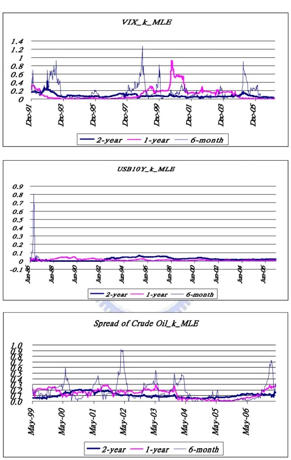
(22) and the log likelihood function is given by. n log Ll = constant − log τ 2 2. ( ).  β β   −κ   X t − µˆ n + − β  − e  X t −1 − µˆ n +  n  κ κ     −∑ 2 2τ t =1. 2. (11). The Maximum Likelihood Estimators (MLE) of κ and σ 2 for the O-U process with linear trend mean are l = − log(s l ) κˆ MLE. σˆ. 2,l MLE. =. (. l 2κˆ MLE.   −κˆ l  β β  X t − µˆ n + l − β  − e MLE  X t −1 − µˆ n + l ∑ κˆ MLE κˆ MLE t =1     n. l. n 1 − e −2κˆ MLE. ).   . 2.  n   ∑ ( X t − µˆ n − β )( X t −1 − µˆ n )  where s l = max t =1 ,0  n   ( X t −1 − µˆ n )2   ∑ t =1   Figure 2 shows how the updated estimators for speeds of mean reversion change by using the weekly data of VIX, interest rate of the United States Treasury Benchmark Bond 10-year, and spread between Brent crude oil and West Texas Intermediate crude oil traded in NYMEX. We discuss three different time scales which are 6-month, 1year, and 2-year respectively to estimate the speeds of mean reversion. The fact is that the less recent observations are considered which means the shorter time scale, the faster speed of mean reversion are reflected.. 15.

(23) VIX_k_MLE 1.4 1.2 1 0.8 0.6 0.4 0.2 0. 19 -c eD. 39 -c eD. 59 -c eD 2-year. 79 -c eD. 99 -c eD 1-year. 10 30 -c -c eD eD 6-month. 50 -c eD. USB10Y_k_MLE 0.9 0.8 0.7 0.6 0.5 0.4 0.3 0.2 0.1 0 -0.1. 0 9 n u J. 8 8 n u J. 6 8 n u J. 2 9 n u J. 4 9 n u J. 2-year. 0 0 n u J. 8 9 n u J. 6 9 n u J. 1-year. 2 0 n u J. 6 0 n u J. 4 0 n u J. 6-month. Spread of Crude Oil_k_MLE 1.0 0.9 0.8 0.7 0.6 0.5 0.4 0.3 0.2 0.1 0.0. 99 -y aM. 00 -y aM. 10 -y aM 2-year. 30 -y aM. 20 -y aM. 1-year. 40 -y aM. 50 -y aM. 60 -y aM. 6-month. Figure 2. MLE for Speed of Mean Reversion: Estimators of the updated estimators for speeds of the mean reversion with different time scales by using the VIX series (top), interest rate series of the United States Treasury Benchmark Bond 10 years (middle), and spread between Brent crude oil and. 16.

(24) West Texas Intermediate crude oil traded in NYMEX (bottom). The fact is that the speeds of mean reversion with shorter time scale are almost faster and than longer time scale. And the speed of mean reversion of VIX series and the spread of crude oil series are obviously faster than the interest rate series of the United States Treasury Benchmark Bond 10 years. In particular, the speeds are all zeroes which mean that there is no evidence for mean reversion since 1986 with shortest time scale.. We utilize a Chi-Square test for the presence/absence of a mean reversion effect. The O-U process is no longer mean reverting when κ = 0 . We wish to test precisely the null hypothesis of no mean reversion ( Η 0 : κ = 0 ) against the alternative of mean reversion ( Η 1 : κ > 0 ).The LR statistic Λ ( X ) can be shown that Λ( X ) =. { ( {(. ). } }. (. ). sup{L0 (θ | X ) : θ ∈ Θ 0 } sup L0 σ 2 | X : θ ∈ Θ 0 L0 σˆ 02 | X = = . 2 sup{L(θ | X ) : θ ∈ Θ} sup L κ , σ 2 | X : θ ∈ Θ L κˆ MLE , σˆ MLE |X. ). (. ). And the test statistic − 2 log Λ will be asymptotically χ 2 distributed with degree of freedom equal to the difference in dimensionality of Θ and Θ 0 . Therefore, − 2(log L0 − log L ) ~ χ 2 (1). The log likelihood function for the O-U process with constant mean under the null hypothesis is log Lc0 = constant −. n (X − X ) n log σ 02,c − ∑ t 2,ct −1 2 2σ 0 t =1. (. ). 2. (12). and the MLE σˆ 02,c of σ 02,c under Η 0 is n. ∑ (X σˆ 02,c =. − X t −1 ). t. 2. t =1. .. n. By the equations (10) and (12), we can obtain that. (. [. ). (. ). ˆc. )]. (. 2 ,c c − 2 log Lc0 − log Lc = n log σˆ 02,c − log σˆ MLE − log 1 − e − 2κ MLE + log 2κˆ MLE +n. −. 2κˆ. (. c MLE. 2,c σˆ MLE 1− e. ) ∑ [( X n. c − 2κˆ MLE. ˆc. t. ]. − µˆ n ) − e −κ MLE ( X t −1 − µˆ n ). 2. t =1. The log likelihood function for the O-U process with linear trend mean under the null hypothesis is. 17.

(25) n ( X − X t −1 − β ) n log Ll0 = constant − log σ 02,l − ∑ t 2 2σ 02,l t =1. ( ). 2. (13). and the MLE σˆ 02,l of σ 02,l under Η 0 is n. ∑ (X σˆ 02,l =. t. − X t −1 − β ). 2. t =1. .. n. By equations (11) and (13), we can obtain that. (. [. ). (. l. ). (. )]. 2 ,l l − 2 log Ll0 − log Ll = n log σˆ 02,l − log σˆ MLE − log 1 − e − 2κˆ MLE + log 2κˆ MLE +n. −. l 2κˆ MLE. (. 2 ,l σˆ MLE 1 − e − 2κˆ. l  β β   −κˆ MLE   X t −1 − µˆ n +  ∑  X t − µˆ n + κ − β  − e κ    t =1 . n. l MLE. ). 18. 2.

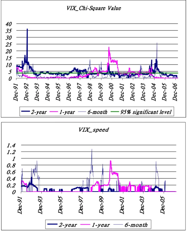
(26) VIX_Chi-Square Value 40 35 30 25 20 15 10 5 0. 19 -c e D. 29 -c e D. 39 -c e D. 2-year. 49 -c e D. 59 -c e D. 69 -c e D. 79 -c e D. 1-year. 89 -c e D. 99 -c e D. 6-month. 00 -c e D. 10 -c e D. 20 -c e D. 30 -c e D. 40 -c e D. 50 -c e D. 60 -c e D. 95% significant level. VIX_speed 1.4 1.2 1 0.8 0.6 0.4 0.2 0. 19 -c eD. 39 -c eD. 59 -c eD 2-year. 99 -c eD. 79 -c eD. 1-year. 10 -c eD. 30 -c eD. 50 -c eD. 6-month. Figure 3. Chi-Square Test for VIX: Set the Chi-Square test for the presence of mean reversion effect with different time scales by using VIX weekly data from 1990 to 2007. The results show that mean reversion phenomenon is significant but the speeds of mean reversion are slower with longer time scale. And the mean reversion is not always significant, but recurring, and the speeds of mean reversion are also clearly faster with shorter time scale.. 19.

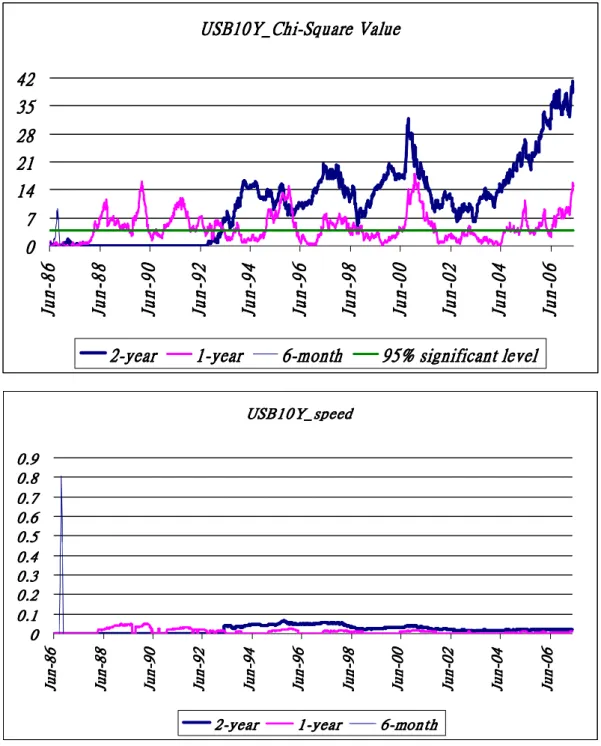
(27) USB10Y_Chi-Square Value 42 35 28 21 14 7 0 6 8 n u J. 8 8 n u J. 0 9 n u J. 2-year. 4 9 n u J. 2 9 n u J. 1-year. 6 9 n u J. 8 9 n u J. 6-month. 0 0 n u J. 2 0 n u J. 4 0 n u J. 6 0 n u J. 95% significant level. USB10Y_speed 0.9 0.8 0.7 0.6 0.5 0.4 0.3 0.2 0.1 0. 6 8 n u J. 8 8 n u J. 0 9 n u J. 2 9 n u J. 4 9 n u J. 2-year. 6 9 n u J. 1-year. 8 9 n u J. 0 0 n u J. 2 0 n u J. 4 0 n u J. 6 0 n u J. 6-month. Figure 4. Chi-Square Test for Interest Rate of U.S. Treasury Bond 10-Year: Set the Chi-Square test for the presence of mean reversion effect with different time scales by using United States Treasury Benchmark Bond 10-year weekly data from 1984 to 2007. The results show that mean reversion is mostly higher significant but the speeds of mean reversion are slow, not exceeding 0.1, with longer time scale. On the contrast, the mean reversion phenomenon is mostly insignificant, but the speeds of mean reversion in 1986 is nearly eight times faster, about 0.8, with short time scale than which with longer time scale.. 20.

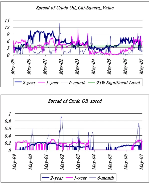
(28) Spread of Crude Oil_Chi-Square_Value 15 12 9 6 3. 2-year. 1-year. 6-month. May-07. May-06. May-05. May-04. May-03. May-02. May-01. May-00. May-99. 0. 95% Significant Level. Spread of Crude Oil_speed 1 0.8 0.6 0.4 0.2. 2-year. 1-year. May-07. May-06. May-05. May-04. May-03. May-02. May-01. May-00. May-99. 0. 6-month. Figure 5. Chi-Square Test for Spread of Crude Oil between Brent and WTI: Set the Chi-Square Test for the presence of mean reversion effect with different time scales by using weekly data of spread between Brent crude oil and West Texas Intermediate crude oil from 1997 to 2007. The results are similar to the series of VIX, which also show that mean reversion phenomenon is mostly significant but the speeds of mean reversion are slower and smoother with longer time scale. And the mean reversion phenomenon is not always significant, but recurring and the speeds of mean reversion are also faster with shorter time scale.. 21.

(29) V.. Conclusions The existence of various types of mean reverting features in asset yields or returns. does not in any way contradict the assumption that markets are efficient. In this paper, we have discussed various other forms of mean reversion, proposed a formal definition of what most investment practitioners and scholar seem to mean by “mean reversion” and estimated the level and speed of mean reversion by using EWMA and MLE respectively. And we realize that the mean reversion is affected by various time scales. Many authors have investigated mean reversion based on the infinite time. Actually, investment practitioners are interested in a variation of underlying asset price at finite time, neither instantaneous nor infinite time. Therefore, we use three different finite time scales which are 6-month, 1-year, and 2-year to investigate the phenomenon of mean reversion. We find out that the speeds of mean reversion are faster with shorter time scale than longer time scale. There is strong evidence for mean reversion in VIX (Volatility Index) and spread between Brent crude oil and West Texas Intermediate (WTI) crude oil, and there are recurring periods where mean reversion is highly significant. However, for the data of USB10Y (United States Treasury Benchmark Bond 10-year), there is strong evidence for mean reversion with longer time scale, but weak evidence with shorter time scale. In this paper, we only discuss the locally constant and linear trend mean models. Manzan (2005) analyzes the annual stock prices data from 1871 until 2003 to show that there is significant evidence to support a nonlinear model in which the speed of mean reversion increases when deviations get large. This confirms previous analysis using nonlinear adjustment models, such as Gallagher and Taylor (2001), Schaller and van Norden (2002), and Psaradakis et al. (2004). The issue of nonlinear mean reversion is worth investigating on future researches.. 22.

(30) Reference Bessembinder, H., Coughenour, J.F., Seguin, P.J., and Smoller, M.M., 1995, “Mean Reversion in Equilibrium Asset Prices: Evidence from the Futures Term Structure,” Journal of Finance, 50, 361-375. Bollerslev, T., 1986, “Generalized Autoregressive Conditional Heteroscedasticity,” Journal of Econometrics, 31, 307-327. Bonomo, M., and Garcia, R., 1994, “Can a Well-Fitted Equilibrium Asset-Pricing Model Produce Mean Reversion?” Journal of Applied Econometrics, 9, 19-29. Brown, R.G.., 1962, “Smoothing, Forecasting and Prediction of Discrete Time Series,” Prentice-Hall, Englewood Cliffs, NJ. Cox. J.C., Ingersoll, J.E., and Ross, S.A., 1985, “A Theory of the Term Structure of Interest Rates,” Econometrics, 53, 385-407. Cox. J.C., and Ross, S.A., 1976, “The Valuation of Options for Alternative Stochastic Processes,” Journal of Financial Economics, 3, 145-166. Dimson, E., Marsh, P., and Staunton, M., 2003, “Global Investment Returns Yearbook 2003,” Published by ABN AMRO ISBN 0-9537906-3-0. Exley, J., Mehta S., and Smith A., 2004, “Mean Reversion” presented to Faculty & Institute of Actuaries Finance and Investment Conference Brussels. Fama, E.F., and French, K.R., 1988a, “Business Cycles and the Behavior of Metals Prices,” Journal of Finance, 43, 1075-1093. Fama, E.F., and French, K.R., 1988b, “Permanent and Temporary Components of Stock Prices,” Journal of Political Economy, 96, 246-273. Gallagher, L.A. and Taylor, M.P., 2001, “Risky Arbitrage, Limits of Arbitrage, and Nonlinear Adjustment in the Dividend-Price Ratio,” Economic Inquiry, 39, No. 4, 524-536. Heston, S., 1993, “A Closed-Form Solution for Options with Stochastic Volatility with Applications to Bond and Currency Options,” Review of Financial Studies, V6, N2, 327-343.. 23.

(31) Holt, C.C., 1957, “Forecasting Trends and Seasonals by Exponentially Weighted Moving Averages,” O. N. R. Memorandum, No. 52, Carnegie Institute of Techology. Hull, J. and White, A., 1990, “Pricing Interest-Rate-Derivatives Securities,” Review of Financial Studies, V3, N4, 573-592. Jegadeesh, N., 1991, “Seasonality in Stock Price Mean Reversion: Evidence from the U.S. and the U.K.,” Journal of Finance, 46, 1427-1444. Kocagil, A.E., Swanson, N.R., and Zeng, T., 2001, “A New Definition for Time-Dependent Price Mean Reversion in Commodity Markets,” Economics Letter, 71, 9-16. Lee, P., 1991, “Just How Risky Are Equities Over the long Term?” Sample Inn Actuarial Society paper, 24th. Lo, A.W., and MacKinlay, C., 1988, “Stock Market Prices do not Follow Random Walk: Evidence from a Simple Specification Test,” Review of Financial Studies, 49, 479-513. MacKinlay, C., and Ramaswamy, K., 1988, “Index-Futures Arbitrage and the Behavior of Stock Index Futures Prices,” Review of Financial Studies, 1, 137-158. Manzan, S., 2005, “Nonlinear Mean Reversion in Stock Prices,” Center for Nonlinear Dynamics in Economics and Finance (CeNDEF), Department of Quantitative Economics, University of Amsterdam. Poterba, J., and Summers, L., 1988, “Mean Reversion in Stock Prices: Evidence and Implications,” Journal of Financial Economics, 22, 27-59. Psaradakis, Z., Sola, M. and Spagnolo, F., 2004, “On Markov Error-Correction Models, with an Application to Stock Prices and Dividends,” Journal of Applied Econometrics, 19, 69-88. Ramsay, J.O., and Silverman, B.W., 2002, “Applied Functional Data Analysis: Methods and Case Studies,” Published by New York Springer-Verlag. Richardson, M., 1989, “Temporary Components of Stock Prices: A Skeptic’s View.” Working Paper, Wharton School of Business, University of Pennsylvania. 24.

(32) Schaller, H. and van Norden, S., 2002, “Fads or Bubbles?” Empirical Economics, 27, 335-362. Vasicek, O. A., 1977, “An Equilibrium Characterization of the Term Structure,” Journal of Financial Economics, 5, 177-188.. 25.

(33) Appendix. By equation (3), we let Yt = e κt X t with the initial condition Y0 = X 0 , and get that. dYt = κe κt X t dt + e κt dX t = κe κt X t dt + e κt [κ (µ − X t )dt + σdWt ] = κe κt µdt + e κt σdWt Therefore, t. E (Yt ) = Y0 + µ ∫ κe κs ds 0. (. ). = Y0 + µ e κt − 1. ∴ E ( X t ) = X 0 e −κt + µ (1 − e −κt ) t. Var (Yt ) = σ 2 ∫ e 2κs dWs 0. 2. =. σ (e 2κt − 1) 2κ. σ2 ∴Var ( X t ) = 1 − e − 2κt ) ( 2κ  σ2 X t ~ N  X 0 e −κt + µ 1 − e −κt , 1 − e − 2κt 2κ . (. ). (. ) . Extending the O-U process with linear trend mean, which is dX t = κ (a + β t − X t )dt + σdWt , we let Yt = e κt X t with the initial condition Y0 = X 0 , and get that dYt = κe κt X t dt + e κt dX t = κe κt X t dt + e κt [κ (a + β t − X t )dt + σdWt ] = κe κt (a + β t )dt + e κt σdWt Therefore, t. E (Yt ) = Y0 + ∫ κe κs (a + β s )ds 0. β   = (Y0 + β t ) +  a − + βt  e κt − 1 κ  . (. 26. ).

(34) β   ∴ E ( X t ) = ( X 0 + β t )e −κt +  a − + β t  1 − e −κt κ  . (. ).  β σ2   1 − e − 2κt X t ~ N  ( X 0 + β t )e −κt +  a − + β t  1 − e −κt , 2κ κ   . (. 27. ). (. ) .

(35)