國
立
交
通
大
學
資訊科學與工程研究所
碩
士
論
文
在數量極大的程式碼中解決測試覆蓋度的
最佳化問題
Test Coverage Optimization Problems with
Large Code Size
研 究 生:周其衡
指導教授:林盈達 教授
在數量極大的程式碼中解決測試覆蓋度的最佳化問題
Test Coverage Optimization Problems with Large Code Size
研 究 生:周其衡 Student: Chi-Heng Chou
指導教授:林盈達 Advisor: Dr. Ying-Dar Lin
國立交通大學
資訊科學與工程研究所
碩士論文
A Thesis
Submitted to Institutes of Computer Science and Engineering College of Computer Science
National Chiao Tung University in partial Fulfillment of the Requirements
for the Degree of Master
In
Computer Science and Engineering June 2008
HsinChu, Taiwan, Republic of China 中華民國九十七年六月
在數量極大的程式碼中解決測試覆蓋度的最佳化問題
學生: 周其衡
指導教授: 林盈達
國立交通大學資訊科學與工程研究所
摘要
迴歸測試經常執行在主要、次要以及甚至僅更正臭蟲的軟體或韌體的新版本 發行。舉例來說,在思科 IOS 的一部份原始碼中,總共有 2,320 個測試用例用來 檢查 57,758 個函式,若在任一次的新版本發行中,將所有的測試用例執行過, 則需要 36 天。在以前的減少測試演算法的研究中,基於聲明程度的條件/分歧的 測試覆蓋度資訊並無法適用於較大的程式,因此難以套用於真實的產品系統中。 在本文裡,我們將根據某測試用例測到某函式的覆蓋度資訊,致力於開發真實測 試方法。當測試資訊的詳細度從條件/分歧減少為函式時,可降低很多複雜度並 且能夠有好的延展性。首先,我們定義一個測試用例的函式可達度(一個測試用 例可以測到多少百分比的函式)以及一個函式的測試強度(百分之多少的測試用 例可以測到特定函式)。透過這兩個標準,覆蓋度的資訊就可被特徵化。然後我 們透過或不透過安全模式來應用貪婪演算法去選取測試用例,所謂安全模式是 指,凡是含有修改過函式的測試例都會被選取出來。在不使用安全模式的情形 中,從部份 IOS 的平均結果看來,我們能夠減少測試成本(時間)為原本的 1/91。 透過安全模式,降低的比例隨著修改過的函式以及它們的測試強度增加而降低。 大多數的更正臭蟲的新版本發行僅修改一個或很少的函式並且它們的測試強度 很低,在此我們的方法能夠應用的更安全及更有效率。 關鍵字: 迴歸測試,軟體工程,減少測試,測試覆蓋度Test Coverage Optimization Problems with Large Code Size
Student: Chi-Heng Chou
Advisor: Dr. Ying-Dar Lin
Institutes of Computer Science and Engineering
National Chiao Tung University
Abstract
Regression testing is conducted frequently on major, minor, and even bug-fix software or firmware releases. For example, as a part of Cisco IOS source codes with 57,758 functions checked by 2,320 test cases, it requires 36 days if all test cases are run on a release. Previous research works on test reduction algorithms select test cases based on the test coverage information of statement-level conditions/branches and could not scale to larger programs, and thus are difficult to apply in real production systems. In this work, we aim to develop a practical test reduction approach based on the coverage information of which test cases "touch" which functions. Since the granularity of coverage information is reduced from condition/branch to function, the complexity is much reduced and could scale well. We first define function reachability of a test (the percentage of functions that a specific test could touch) and test intensity of a function (the percentage of tests that touch a specific function). With these two metrics, the coverage information is characterized. We then apply greedy algorithms to select test cases, with or without a safe mode that selects all test cases touching modified functions. The results from instrumenting parts of IOS show that we could reduce the test cost (time) to 1/91, on the average, without a safe mode. With a safe mode, the reduction ratio drops as the number of modified functions and their test intensities increase. Numerous bug-fix releases modify only one or very few functions with low test intensity, where our approach can be applied safely and effectively.
Contents
1 INTRODUCTION ... 1
1.1 MOTIVATION ... 1
1.2 RELATED WORKS ... 1
1.3 CONTRIBUTION ... 3
2 NOTATION DEFINITION AND PROBLEMS ... 5
2.1 NOTATION DEFINITION ... 5
2.2 SIX PROBLEMS ... 7
3 DESIGNING SIX ALGORITHMS ... 10
3.1 PDF-SA ALGORITHM ... 10
3.2 CW-NUMMIN,CW-COSTMIN AND CW-COSTCOVB ALGORITHMS ... 10
3.3 CW-COVMAX ALGORITHM ... 13
3.4 CW-COSTMIN-C ALGORITHM ... 14
4 SYSTEM DESIGN AND IMPLEMENTATION ... 16
4.1 TESTING SERVER ... 16
4.2 RFCCONVERTER AND IMPORTER ... 17
4.3 RFCDATABASE ... 17
4.4 RFCVIEWER ... 18
5 EXPERIMENTAL RESULTS ... 19
5.1 CHARACTERISTICS OF THE TEST-FUNCTION MAPPINGS ... 19
5.2 RESULT ANALYSIS ... 23
5.2.1 The impact of different test intensity threshold ... 23
5.2.2 Inside the results ... 24
5.2.3 CW-NumMin and CW-CostMin results ... 25
5.2.4 CW-CostCovB Results ... 25 5.2.5 CW-CovMax Results ... 26 5.2.6 CW-CostMin-C results ... 28 5.2.7 PDF-SA Results ... 29 6 CONCLUSIONS ... 32 7 REFERENCE ... 34
List of Figures
FIGURE 1DEFINITIONS OF VARIABLES ... 5
FIGURE 2DEFINITIONS OF FUNCTIONS ... 6
FIGURE 3PDF-SA ALGORITHM... 10
FIGURE 4CW-NUMMIN,CW-COSTMIN AND CW-COSTCOVB ALGORITHMS ... 12
FIGURE 5CW-COVMAX ALGORITHM... 14
FIGURE 6CW-COSTMIN-C ALGORITHM ... 15
FIGURE 7REGRESSION FUNCTION COVERAGE ARCHITECTURE ... 16
FIGURE 8RFCDATABASE ... 18
FIGURE 9FUNCTION REACHABILITY AND TEST INTENSITY... 20
FIGURE 10DISTRIBUTIONS OF DDTSS ... 21
FIGURE 11SAFE SELECTION... 22
FIGURE 12TS VS.CW-NUMMIN,CW-COSTMIN RESULTS... 24
FIGURE 13EXPLANATION OF THE TYPES OF FUNCTIONS IN CW-NUMMIN ... 25
FIGURE 14CW-COSTCOVB RESULTS ... 26
FIGURE 15CW-COVMAX RESULTS ... 28
FIGURE 16CW-COSTMIN-C RESULTS ... 29
FIGURE 17PDF-SA RESULT ... 30
List of Tables
TABLE 1THE DESCRIPTION OF PROBLEMS ... 8
TABLE 2TEST COVERAGE OPTIMIZING PROBLEMS ... 8
TABLE 3CW-COSTCOVBEXAMPLE ... 13
1 Introduction
1.1 Motivation
During the lifecycle of a large industrial software product, the number of test cases and their complexity increase significantly as new versions of software are constantly released. The developers tend to skip some insignificant test cases and forgo the fault detection opportunities due to the cost of reproducing all the accumulated test cases. The test cases are selected according to their cost and the fault detection opportunities. An array of selection algorithms have been designed based on a variety of models on the relations between the code coverage and fault detection opportunities of test cases. However, these algorithms still demand a large space of database and the long execution time due to the huge number of test cases and functions.
The relationships between test cases and functions are like an interlaced net. The selection of the function involves some test cases, and vice versa. We define the test intensity of a function and the function reachability to explain the relationships between test cases and functions, where the former is the percentage of test cases that cover or invoke the functions, and the latter is the percentage of functions covered by test cases. Through the relationships and different selection requirements, we could find several practical problems with test reduction and solve them.
1.2 Related works
This section discusses the method of choosing suitable test cases to effectively reduce the testing time and the loss of fault detection capability, as well as existing study in reducing the number of test cases. The trade-offs of the number of selected
test cases and fault detection capability are somewhat controversial. For example, Wong et al. [1] concludes that test cases without adding coverage to a test set are likely to have small impact on fault detection capability. However, minimizing test cases is reported to severely compromise the fault detection capability in [2]. Hence, these two papers illustrated that selecting effective test cases with the fault detection capability is important.
Regression testing is conducted frequently on major, minor, and even bug-fix software or firmware releases. It always focuses on the newly modified portion of the source codes, implying that a test case that does not cover any function having been modified since the last regression test will not reveal any new fault, so skipping the test case will not lose the fault detection capability of a new regression round. Hence, each regression testing can detect every fault by test cases. In other words, the new faults should be generated by functions newly introduced or modified since the last regression test. It also means regression testing will not find less new faults by not running the test cases which do not cover modified functions. This assumption is held throughout this thesis.
Reducing the regression testing is a well-known minimal set-cover problem, which is an NP complete problem [1],[3],[4]. According to [3], the reduction includes the test selection problem and the test plan update problem. Since our experiments work on the practical circumstances of the existing automated regression test system and do not have the information of the test plan, here we only investigate the test selection problem that is also called test case reduction problem. The test case reduction problem is clearly defined as follows:
Given: A test suite T, a set of testing requirements {r1,r2,...,rn}, that must be
satisfied to provide the desired test coverage of the program, and subsets {T1,T2,...,Tn}
belonging to Ti covers ri.
Problem: Find a representative set of test cases tj that will satisfy all of the ri's
A number of methods can solve the test case reduction problem in polynomial time, e.g., the greedy heuristic methods [5]-[8], the generic algorithm methods [9],[10][11] and the integer linear programming methods [12]. The greedy heuristic methods are generally better than others [13][14], so our algorithms adopt a greedy heuristic method. The related research about reduction of regression testing also includes prioritizing test cases for regression testing [15], modeling the cost-benefits for regression testing [16] and impact of test case reduction on fault detection capability [1][2][17][18]. We focus only on greedy heuristic methods, which have some different applications. The focus on fault detection capability, especially with the branch coverage, can be seen in [5][6][7]. The hitting set algorithm [5] categorizes test cases in the test suite according to the degree of “essentialness” and selects test cases in the order from most “essential” to least “essential”. The G/GE/GRE algorithms [8] are based on three strategies: essential, 1-to-1 redundant and greedy strategies. However, the previous algorithms do not match our needs exactly. The G algorithms [8] are adapted to new applications to solve the problems we face in the next chapter and the algorithms for these problems in Chapter 3.
1.3 Contribution
This thesis describes the implementation of a database driven test case selection service in an automated regression test production system capable of providing information of code coverage trace and execution time of each test case. The service also imports code modification history from the source control system with the intention to focus on the opportunity of detecting faults caused by newly modified codes. We define two metrics to characterize the coverage information: function
reachability of a test and test intensity of a function. Then we adopt algorithms from previous works to the practical circumstances of the existing automated regression test system, and devise some test case selection strategies for different concerns.
The organization of this paper is as follows. Chapter 2 first defines the notation of selection algorithms and describes the six problems. Next, Chapter 3 describes our designed test case selection strategies adapted to the circumstances of the real life system. Chapter 4 states the implementation of our practical database-driven test case selection services and Chapter 5 provides the experiment environment and results. Finally, Chapter 6 discusses the lessons learned from this exercise and future work.
2 Notation definition and problems
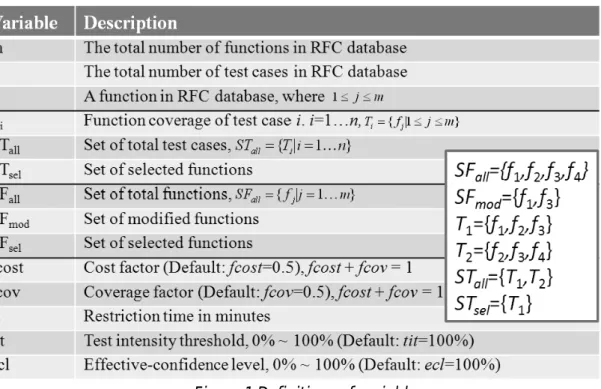
2.1 Notation Definition
Some definitions of variables and functions are tabulated in Figure 1 and Figure 2, respectively. From Figure 1, there are two test cases {T1, T2 } and four functions
SFall={ f1, f2, f3, f4}, with two modified functions, SFmod = {f1 , f3}. When we need to
choose a test case to cover modified functions, the reasonable selection is T1, which
covers f1 and f3. Thus, STsel={T1}. Next, five parameters that are constraints of our
algorithms, such as fcost, fcov, rt, tit and ecl, will be explained further in each algorithm.
Figure 2 Definitions of functions
Figure 2 shows the definition of functions, which are basic components in our algorithms. COST(Ti) returns the execution time of test case Ti. Test case count TC(fi)
returns the number of test cases which cover fi function count FC(Ti) and function
coverage count FCC(SFmod,Ti) both return the number of functions to be covered by
the test case Ti, but FCC(SFmod,Ti) puts special attention on modified functions. Extra
function coverage count EFCC(SFmod,Ti) returns total function count minus function
coverage count. Finally, TFC(STall) and TEFCC(SFmod,STall) return total function
count and total extra function coverage count, respectively. In the CostCovB problem, the cost or extra coverage factor used to decide cost is meaningful or extra coverage. The algorithm of this problem uses CV(SFmod,STall,Ti,fcost,fcov) to choose the most
balancing test case. The detailed definitions of functions are listed in Figure 2. Because CV() is used to select best balancing test case, it should be composed by two parts, cost and coverage, where the former is PARAW(SFmod,Ti) * fcost and the latter is
PARAC(SFmod,STall,Ti) * fcov. fcost and fcov are factors of cost and extra coverage,
respectively. PARAW() returns the percentage of WEIGHT(SFmod,Ti) among total
WEIGHT(SFmod,Ti) and PARAC(SFmod,STall,Ti) returns the percentage of
EFCC(SFmod,Ti) among TEFCC(SFmod,STall).
We define function reachability of a test (FC(Ti)/|SFall|) as the percentage of
functions that a specific test could touch, and test intensity of a function (TC(fi)/|STall|),
as the percentage of tests that touch a specific function. The coverage information is characterized by these two metrics.
2.2 Six Problems
The empirical study we made is on the prevailing Cisco Internetwork Operating System (IOS) which has very huge code size and test cases. Our study is confined to about 50,000 functions and 2,300 test cases that are only a portion of whole system. Each test case operates a series of configuration and testing steps. The runtime of a test case varies from 10 minutes to 100 minutes. Conducting a complete regression testing of 2,300 test cases on a single test platform takes a few weeks, so selecting a small and proper subset of test cases in regression testing can save a lot of time. From the previous assumption, we focus on test cases that cover modified functions. How do we get the minimal number of test cases or minimal cost of test cases with the knowledge of which functions have been modified since the last regression round, or even balance between cost and coverage? Furthermore, with a given limited testing time, how do we get maximal coverage? With a given required level of coverage, how do we get the minimal cost of test cases? How to reduce selecting time of selection algorithms? We summarize the problems in Table 1.
Table 1 The description of problems
Problem Short name Description
The Number-Minimization
Problem NumMin
Given the modified functions to get the minimal number of test cases
The Cost-Minimization
Problem CostMin
Given the modified functions to get the minimal cost of test cases
The Cost and Coverage
Balance Problem CostCovB
Given the modified functions to get the test cases which can balance cost and extra coverage The Coverage-Maximization
Problem CovMax Given the restriction time to get the max coverage The Cost-Minimization with
Confidence Level Problem CostMin-C
Given the effective-confidence level to get the minimal cost of test cases
The Selection Acceleration
Problems SA
Find the infrastructure functions to reduce the functional space
Moreover, executing the test case selection algorithms also takes time, which is a large cost, if requirement is frequently asked. Functions with test intensity over a preset threshold (e.g., 90%) are designated infrastructure functions (TC(fi)/|STall|≧tit).
Removing these functions improves the speed of algorithms. The constraints of the six typical problems and the benefits derived from their respective solutions are tabulated in Table 2.
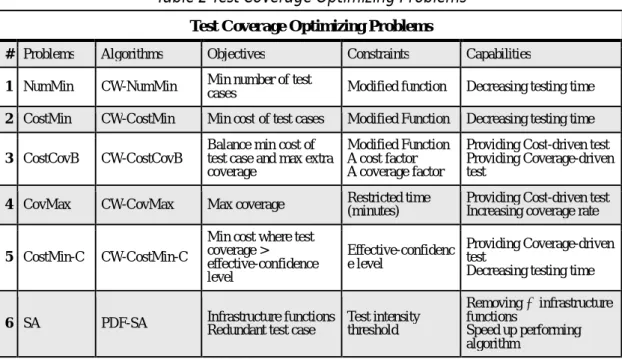
Table 2 Test Coverage Optimizing Problems
Test Coverage Optimizing Problems
# Problems Algorithms Objectives Constraints Capabilities
1 NumMin CW-NumMin Min number of test
cases Modified function Decreasing testing time
2 CostMin CW-CostMin Min cost of test cases Modified Function Decreasing testing time
3 CostCovB CW-CostCovB
Balance min cost of test case and max extra coverage
Modified Function A cost factor A coverage factor
Providing Cost-driven test Providing Coverage-driven test
4 CovMax CW-CovMax Max coverage Restricted time (minutes) Providing Cost-driven test Increasing coverage rate
5 CostMin-C CW-CostMin-C
Min cost where test coverage > effective-confidence level Effective-confidenc e level Providing Coverage-driven test
Decreasing testing time
6 SA PDF-SA Infrastructure functions Redundant test case Test intensity threshold
Removing —infrastructure functions
Speed up performing algorithm
In the NumMin and CostMin problems, given a set of modified functions, we need to find the minimal number or cost of test cases, subject to the constraint that each modified function in the set must be called at least once. After solving these two problems, testing time of regression testing could be reduced.
In the CostCovB problem, in order to balance cost and coverage, we judge which factor, cost or coverage, is more important with the set of modified functions. The solution provides a guide between cost-driven and coverage-driven tests.
In the CovMax problem, given a constant total test time restriction, the test cases with maximal coverage and the cheapest cost is chosen to provide a cost-driven test strategy.
In the CostMin-C problem, an effective-confidence level as an alternative measure of coverage is adapted. The coverage over only the functions registered in RFC database, as in contrast to coverage over all functions is called
effective-confidence level. Due to large code size, the mapping of the functions, which
is unreachable by any test case, and test cases is so large that performing an algorithm for these useless mapping only increases cost without improving accuracy. Thus, RFC database only stores the mapping of reachable functions and test cases, and this is why effective-confidence level is instead of coverage level. Solution of this problem could provide a coverage-driven test strategy which also decreases testing time.
In the SA problem, owing to speed up other algorithms, execution of the selection algorithms do consider the infrastructure functions with different test intensity criteria. For example, with the 100% test intensity threshold, the functions covered by every test case can be skipped. Hence, when performing algorithms, the considered functions in selection algorithms becomes small and each algorithm becomes faster. By controlling the size of the infrastructure function set, the algorithms can speed up their testing.
3 Designing Six Algorithms
The six practical problems and designed strategies are shown in Table 2. There are two categories of algorithms: the PDF-SA algorithm and the prefix of the CW algorithms.
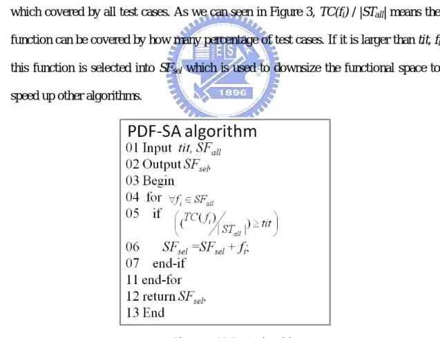
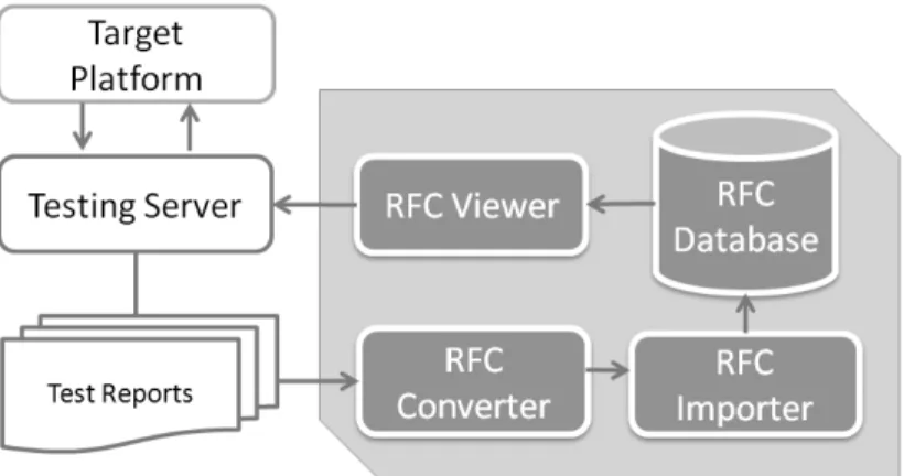
3.1 PDF-SA algorithm
In order to reduce the number of function concerned in selection algorithms, the number of test cases to cover each function will be calculated. The tit is the test intensity threshold, a kind of metric; to describe a degree of how many percentages of test cases can cover each function. For example, if tit=100%, we remove the functions which covered by all test cases. As we can seen in Figure 3, TC(fi) / |STall| means the
function can be covered by how many percentage of test cases. If it is larger than tit, fi
this function is selected into SFsel which is used to downsize the functional space to
speed up other algorithms.
Figure 3 PDF-SA algorithm
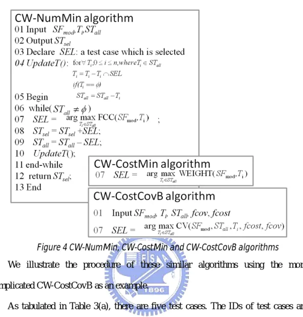
3.2 CW-NumMin, CW-CostMin and CW-CostCovB algorithms
(CW). The CW-NumMin, CW-CostMin and CW-CostCovB algorithms have similar structure except the mechanism of selecting the CW value, as listed in Figure 4. The CW-NumMin algorithm uses FCC(SFmod,Ti) as CW value because larger
FCC(SFmod,Ti) means a larger coverage in the test cases. After selecting one test case
into STsel, it’s necessary to update STall. Next, using UpdateT() to remove the test
cases which do not cover any functions. Because when a test case does not have any extra coverage, it should be removed from STall. And then continue to perform this
loop until STall = null. The CW-CostMin algorithm uses WEIGHT(SFmod,Ti) as CW
value. Larger WEIGHT(SFmod,Ti) means more coverage under the same cost. In the
other words, larger WEIGHT(SFmod,Ti) means cheaper, so the WEIGHT(SFmod,Ti) is
token as CW value by the CW-CostMin algorithm. In the CW-CostCovB algorithm uses CV(SFmod,STall,Ti,fcost,fcov) as CW value. In chapter 2.1, we have showed that
the larger CV(SFmod,STall,Ti,fcost,fcov) means this test case can have better balance
Figure 4 CW-NumMin, CW-CostMin and CW-CostCovB algorithms
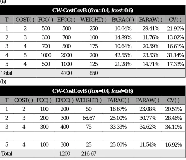
We illustrate the procedure of these similar algorithms using the more complicated CW-CostCovB as an example.
As tabulated in Table 3(a), there are five test cases. The IDs of test cases are from 1 to 5 and execution times are 2, 3, 4, 5 and 4 minutes, respectively. These test cases could cover the number of 500, 300, 700, 1,000 and 500 modified functions and also cover the extra functions with the number of 500, 700, 500, 2,000 and 1,000, respectively. The factors for the cost and the extra coverage are fcov=0.4 and
fcost=0.6.
At the beginning, we get the value of WEIGHT(), FCC()/COST(), from each test case. For example, WEIGHT() of test case 1 is 500/2=250. The other four test cases get the value of WEIGHT() in the same way. Then we sum the value of WEIGHT() and the value of EFCC() for five test cases, separately. The total value of WEIGHT() is 850 and the total value of EFCC() is 4,700. Next, we get the value of PARAC() and
EFCC() = 500/4,700 = 10.64% and PARAW() = WEIGHT() / Total WEIGHT() =
250/850 = 29.41%. That means the percentage of the extra coverage and the percentage of cost of test case 1 is 10.64% and 29.41% among all test cases, respectively. Therefore, the value of CV() can be calculated by PARAC()*fcov +
PARAW()*fcost = 10.64%*0.4 + 29.41%*0.6 = 21.90%. As illustrated in Table 3(a),
the test case 4 has the largest value of CV(). Hence, the test case 4 is chosen as the selected test case and then the values of FCC() and EFCC() are updated by recalculating them after removing the functions covered by test case 4. The above steps are repeated until the selected test cases can cover all modified functions.
Table 3 CW-CostCovB Example
(a)
CW-CostCovB (fcov=0.4, fcost=0.6)
T COST( ) FCC( ) EFCC( ) WEIGHT( ) PARAC( ) PARAW( ) CV( )
1 2 500 500 250 10.64% 29.41% 21.90% 2 3 300 700 100 14.89% 11.76% 13.02% 3 4 700 500 175 10.64% 20.59% 16.61% 4 5 1000 2000 200 42.55% 23.53% 31.14% 5 4 500 1000 125 21.28% 14.71% 17.33% Total 4700 850 (b)
CW-CostCovB (fcov=0.4, fcost=0.6)
T COST( ) FCC( ) EFCC( ) WEIGHT( ) PARAC( ) PARAW( ) CV( )
1 2 100 200 50 16.67% 23.08% 20.51% 2 3 200 300 66.67 25.00% 30.77% 28.46% 3 4 300 400 75 33.33% 34.62% 34.10% 5 4 100 300 25 25.00% 11.54% 16.92% Total 1200 216.67
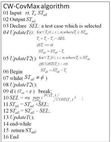
3.3 CW-CovMax algorithm
In the CW-CovMax algorithm, as listed in Figure 5, cost is the constraint. The idea is the same as the CW-CostMin, but the target is all functions, rather than modified functions. Hence, FC(Ti)/COST(Ti) is used as CW value. Because the test
time of Ti is larger than the restriction time, Ti has no change to be selected test case.
Hence, we use UpdateT2() to remove test cases, which testing time are greater than the restriction time, before selecting the test cases.
Figure 5 CW-CovMax algorithm
3.4 CW-CostMin-C algorithm
CW-CostMin-C algorithm extends from the CW-CostMin algorithm, as listed in Figure 6. FC()/COST() is used as CW value. The loop terminates when STall is null or
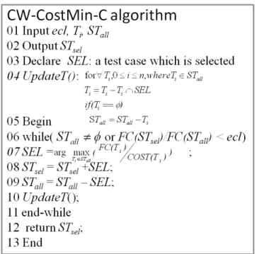
4 System Design and Implementation
In the implementation, we designed a Regression Function Coverage Architecture (RFCA) illustrated in the right portion of Figure 7 to solve these problems. There are four components: RFC Converter, RFC Importer, RFC Database and RFC Viewer. After performing regression test, there are test reports generated by testing tools in the testing server. RFCA imports these test reports into the RFC database, configures to run test case selection algorithms, and then replies a list of selected test cases to test the server through the RFC Viewer. The input of RFCA is the output of the testing server. Therefore, we first introduce the testing server.
Figure 7 Regression Function Coverage Architecture
4.1 Testing Server
Before performing regression testing, we should instrument the target platform by the Testwell CTC++[19] first, owing to display which portion of source is covered. Test cases are executed on the test sever to test the target platform. When the target platform is tested, the testing server will generate raw test reports, which only contain coverage information of all functions, including reachable and unreachable functions by a test case, in the instrumented target platform. Because the information of unreachable function cannot give any help in the selection algorithms, it should be
removed from test reports. After the simple transformation of test reports by the testing server, the refined test reports are generated without the information of unreachable functions. After that, the testing server outputs the refined test reports to RFC Converter. It also outputs the file-list and status files, where the former records each test case belonging to which test area1, and the latter records the execution time of test cases. These files are used to construct the schema of test cases in RFC database.
4.2 RFC Converter and Importer
RFC Converter combines the file-list, status files and test reports into complete test reports, called test summary files. Each test summary file contains complete function coverage information and the information of testing environment. Next, RFC Importer reads these test summary files, parses these and records the corresponding field in RFC database.
4.3 RFC Database
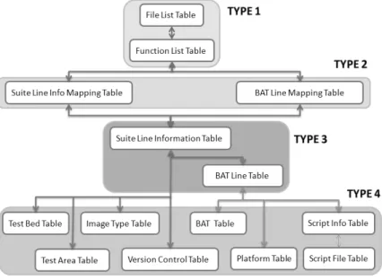
RFC Database has 14 schema, which categorized as four categories from type 1 to type 4, as listed in Figure 8. The type 1 schema stores information of functions, including file name, file path and function name. The type 2 schema stores the relationships between functions and test cases by only two IDs, the function id and the test case id. Because the size of type 2 schema grows fast and is very large. In type 3 schema, it stores the relationship between each test report and the corresponding testing environment. The type 4 schema records the related information about testing environment. These schemas could help to reduce the number of test cases by filtering the testing environment. For example, when target platform is version A and image
1
Test area includes MPLS, VPN and etc. in Automated Test Center (ATC) which is a central Cisco test team
type B, only the corresponding test cases under these two constraints is selected to perform selection algorithm.
Figure 8 RFC Database
4.4 RFC Viewer
RFC Viewer has two steps to generate a list of selected test cases. First, a client inputs the modified function list and the parameters of selection algorithms from clients including fcost, fcov, rt, tit and ecl. At same time, RFC Database generates the execution time file, the list of test intensity of functions and test case files. The execution time file records the execution time of each test case. The list of test intensity of functions used to remove infrastructure functions from certain test intensity threshold. The test case files contain the mapping from test case ID to function ID. The reason of using temporary files instead of exporting data from RFC Database is to speed up the process of RFC Viewer. If someone is trying to read data from RFC Database and the other plans to execute algorithms from RFC Database, RFC database becomes slow. Finally, the list of selected test cases is generated by the selection algorithms discussed above.
5 Experimental Results
5.1 Characteristics of the Test-Function Mappings
Our experiment platform uses a personal computer, which has AMD Athlon 64 Processor 3800+ 2.41GHz with 3GB RAM and Microsoft Windows XP Professional SP2. The experiments are executing on this platform.
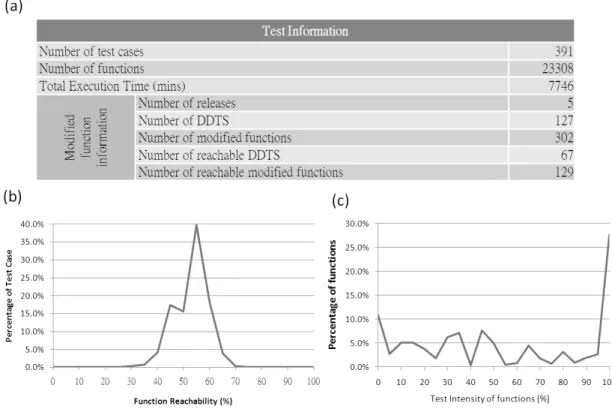
We choose MPLS test area as our experiment target because it has more test cases than other test areas. As tabulated in Figure 9(a), there are 391 test cases in MPLS test area. They cover 23,308 functions and their total execution time is 7,746 minutes. The function reachability of 391 test cases is depicted in Figure 9(b). Because the test cases execute a series of procedures, they have really high function reachability. Most test cases can cover about 40% to 60% functions, meaning that most test cases have the 40% to 60% function reachability and also implying that a few selected test cases may cover total functions. The test intensity of 23,308 functions can be seen in Figure 9(c). There are over 25% functions can be covered by all test cases. The distribution of test intensity of functions is average.
Figure 9 Function Reachability and Test Intensity
There are five releases and each release contains several DDTSs2, which are bug tracking records, in this experiment. There are total 127 DDTSs which contain 302 modified functions. However, MPLS only covers 67 DDTSs which have 129 modified functions, as illustrated in Figure 9(a). Next, we try to explain the information of DDTS in detail.
As illustrated in Figure 10(a), five releases, which are 124-13.12, 124-13.13, 124-13.14, 124-13.15, 124-13.16, contain 13, 16, 24, 3 and 11 DDTSs, respectively. That means the distributions of bug tracking records in each release is nonuniform. At same time, over 65% DDTSs only modify 1 function which is shown in Figure 10(b). Furthermore, the test intensity of three types, which are percentage of DDTS with FC=1, percentage of functions and percentage of DDTS, range from 0% to 100% and 100% test intensity of theirs are 25%~30% as listed in Figure 10(c). It implies that
2
25%~30% DDTSs are covered by all test cases. We will use the information of distributions of DDTSs to explain why safe method is not enough.
Figure 10 Distributions of DDTSs
The safe method selects all test cases that can cover modified functions. And then it is performed to explain the cost of selected test cases from the above distribution of DDTSs. At first, the percentage of TCsel/TC, FC/TFC and
COSTsel/COST of each DDTS with the safe method are sorted by percentage of
TCsel/TC. As listed in Figure 11, the average cost of DDTSs is still high. The cost in
almost DDTSs is greater than 40%. Only 4 DDTSs can get smaller cost. In other words, 94% DDTS do not have good cost down with safe method. Because 94% DDTSs are covered by too many test cases or covered by the test cases which cost high. Hence, the safe selection method is not enough. We need to further reduce the cost.
Figure 11 Safe selection
Because the selection algorithms will use different test intensity of functions to compare the effective of speedup, the PDF-SA experiment is first conducted to understand the distribution of infrastructure functions in different test intensity of functions. The scenario of each experiment can be seen in Table 4. We choose the test intensity threshold with NA, 80, 90 and 100, to see the effect of different test intensity of functions to each selection algorithm. With different test intensity of functions, we can prove that the selection algorithms without considering the infrastructure functions are faster. Next, each selection algorithm is performed. In the CW-NumMin and the CW-CostMin algorithms, we want to observe that how many selected test cases and cost can be reduced. In the CW-CostCovB algorithm, the effects of fcov and
fcost are investigated. In the CW-CovMax algorithm, 500 and 1,000 minutes are
selected as restriction time due to the execution time of each test case is between 10 to 100 minutes. Finally, the speedup of the different test intensity thresholds will be compared in the PDF-SA algorithm.
Table 4 Summarization of Scenarios
Steps Algorithms Test Intensity
Threshold Other Parameters 1 PDF-SA 0, 5, …, 100
2 CW-NumMin NA, 80, 90, 100
3 CW-CostMin NA, 80, 90, 100
4 CW-CostCovB NA, 80, 90, 100 fcov = {0, 0.1, …, 1}
5 CW-CovMax NA, 80, 90, 100 rt = {500, 1000}
6 CW-CostMin-C NA, 80, 90, 100 ecl = {10, 20, …, 100}
5.2 Result Analysis
5.2.1 The impact of different test intensity threshold
In the following testing, we choose a symbol of CW to represent the situation of consider all functional space and tit to represent test intensity threshold. For example, CWtit100 is a case which does not consider 100% test intensity of functions.
The goals of the CW-NumMin and the CW-CostMin algorithm choose the minimal test cases and the minimal cost, respectively. At the beginning, we have to analyze does different tit have different impact to cost and coverage in the experiments, as illustrated in Figure 12 (a). In the CWtit100, CWtit90, CWtit80 and CW of
the CW-NumMin, the difference only appears in EFCC/TFC value. Because the effect of without considering infrastructure functions has less impact. We only explain the experiment results in CWtit100 scenario in the following selection algorithm. However,
why the value of EFCC/TFC has difference with 27.59% (92.41%-64.82%) in the CWtit100 and CW of the CW-NumMin? We have to explain the significance in these
Figure 12 TS vs. CW-NumMin, CW-CostMin results
5.2.2 Inside the results
In Figure 13, in order to explain how many types of function exist in a complete functional space, we take CW and CWtit100 in the CW-NumMin algorithm as an
example. First, the total coverage can be divided as two parts, one is FC/TFC and the other one is (TFC-FC)/TFC. FC/TFC means the degree of coverage. In contrary, the (TFC-FC)/TFC means the degree of non-coverage. The FC/TFC has 92.96% in the CW. Furthermore, FC/TFC is composed of three parts: EFCC/TFC, Infrastructure functions / TFC and Modified functions / TFC. The corresponding percentage is 92.41%, 0% and 0.55% respectively. However, the modified functions have 302 numbers and account for 1.295% of all functions. But it only has 0.55% in Figure 13. Because not every modified function can be covered in MPLS test area. There are 129 modified functions real in MPLS test area and account for 0.55% only.
The percentage of FC/TFC is 92.62% in CWtit100. EFCC/TFC, Infrastructure
functions / TFC and Modified functions / TFC account for 64.82%, 27.59% and 0.55%, respectively. However, the percentage of infrastructure functions is not equal to 27.73% where we discussed above. Because there is 0.14% functions are infrastructure functions and modified functions at the same time. Whatever the
functions belong to infrastructure functions or not in our selection algorithms, we should consider the modified functions into algorithms. That’s why the infrastructure functions only reduce 27.5% functional space.
Figure 13 Explanation of the types of functions in CW-NumMin
5.2.3 CW-NumMin and CW-CostMin results
Next, we observe the CWtit100 in the CW-NumMin algorithm as illustrated in
Figure 12(a). If we select 2.56% of all test cases, all the modified functions can be covered. And it also provides 64.82% extra function coverage count and cost 2.32% of original tests. As illustrated in Figure 12(b), the CWtit100 only needs to select 2.56%
test cases to cover all modified functions in the CW-CostMin algorithm. It also provides 62.3% extra function coverage count and cost 1.10% of original tests. We pick up TCsel/TC and COSTsel/COST from Figure 12(a) and normalize as traditional
selection (TS) in Figure 12(b). In the CWtit100 of the CW-NumMin and the
CW-CostMin algorithms, it only need 1/39 and 1/39 test case of TS, and 1/43 and 1/91 cost of TS, respectively. Our selection algorithms can reduce a lot of test cases and costs, obviously. Furthermore, because the CW-CostMin always selects the cheapest test case and the CW-NumMin always selects the test case with largest coverage, the cost of the CW-CostMin is less than the one of the CW-NumMin.
5.2.4 CW-CostCovB Results
In the CW-CostCovB algorithm, we provide a cost-driven and coverage-driven algorithm. We judge which factor, cost or coverage, is more important. The parameter
fcov and fcost is the factor of extra coverage and cost, respectively. When fcov is
higher than fcost, it means that extra coverage is emphasized. We analyze every kind of parameters where fcov from 0, 0.1, … 1, in other words, fcost from 1, 0.9, … 0. In the curve of EFCC/TFC as illustrated in Figure 14(a), fcov=0 and fcost=1 means we emphasize cost most. When we use fcost=1, the CW-CostCovB becomes the CW-CostMin. The selected test cases can provide 62.3% extra coverage. However, from fcov=0 to fcov=1, the extra coverage only falls in 62% to 69% coverage. The extra coverage is hard to have over 69% coverage because the coverage of infrastructure functions have about 27% coverage. In additional, the curve of COSTsel/COST grows a lot when fcov from 0.3 to 0.4 and spends 1% cost more. The
cost only locates on 1% to 3% whatever the selection of fcov. The cost is small but still has large extra coverage, because these selected test cases have large function reachability and have small cost at same time. To compare the difference of emphasis in extra coverage and cost, we choose the extreme result which is fcov=0 and fcov=1, as illustrated in Figure 14 (b). Based on fcov=0, to normalize these two results. For an extra 6% coverage (96.25%-90.44%), we pay a cost of 2.6 times (1.097%→2.853%) and select the test cases of 1.2 times. Hence, we recommend the fcov=0 is better choice in the MPLS test area.
Figure 14 CW-CostCovB results
In the CW-CovMax algorithm, we provide a cost-driven method. The client can perform different selection policies by different restriction time. We use 500 and 1,000 minutes here. As illustrated in Figure 15 (a), there is 99.63% coverage in rt=500 and 100% coverage in rt=1,000. We can see that in order to improve a little bit coverage would pay a lot of cost. Based on rt=500, we normalize rt=1,000 as depicted in Figure 15 (b). The coverage only improves 0.37% in rt=1,000, but it needs to select 1.44 times test cases and 1.98 times cost. It means that only few parts of functions are covered by a certain test case. In order to improve the coverage from 99% to 100%, we need to select many test cases. It concluded that choosing appropriated restriction time is important. In additional in Figure 15 (a), the 15.58% test cases can reach 100% coverage. In other words, the functions which are covered by all test cases can also be covered by other 15.58% test cases. There are two possibilities to explain this. First, there are old version test cases. We add new test cases without deleting old test cases. The functions which can be covered by old version test cases also can be covered by new version test cases. Next, the granularity of coverage is big. When a function is covered by a certain test case, we mark this function as covered. In actually, some test cases may use to test the different parts of the function. Because the testing resource is limited and the reason of easy to manage, we use the function coverage as coverage criteria. The fault detection capability may be decreased if choosing a bigger granularity. We only provide a case study. The real impact of reducing test cases on fault detection capability in our system with large code size would be future works.
Figure 15 CW-CovMax results
5.2.6 CW-CostMin-C results
In the CW-CostMin-C algorithm, we provide a coverage-driven method. The client can get the minimal cost according to the sufficient coverage. This algorithm extends from CW-CostMin algorithm. We select the cheapest test cases in each step until the sufficient coverage is reached. Each step uses the CW-CostMin algorithm. Obviously, when the test cases in n={0,10,…,90} and ecl=n+10, they must contains test cases in ecl=n. We perform the algorithm from ecl=10 to ecl=100. In Figure 16 (a), the coverage is 68.82% from ecl=10 to ecl=60. Because when we select a test case in ecl=10, it already provides 68.82% coverage. Until ecl=70, it just selects new test cases. Because the huge changes of cost from ecl=90 to ecl=100, we focus on this division. We need to select 1.79% test cases and cost 0.529% in ecl=90. We also need to select 15.85% test cases and cost 12.74% in ecl=100. Based on ecl=90, we normalize ecl=100, as illustrated in Figure 16 (b). Increasing the 8.85 times test cases and 24.08 times cost from coverage 90% to 100%. It also means that there is only few functions are covered by certain test cases. Hence, the cost grows a lot when coverage from 90% to 100%. It is important to choose appropriate ecl.
Figure 16 CW-CostMin-C results
5.2.7 PDF-SA Results
After explaining the results of all algorithms, we focus on the PDF-SA algorithm to see the improvement in each algorithm. The Probability Density Function (PDF) and Cumulative Density Function (CDF) of test intensity of functions are shown in Figure 17 (a). In order to analyze and draw figure easily, different values of test intensity of functions are aggregated into a separate division. For example, 20% means the test intensity of functions is from greater than or equal to 20% to less than 25%. Observed from Figure 17 (a), the distribution of PDF is irregular. 0% and 100% test intensity of functions are larger than others, meaning that two large portions of functions are covered by many test cases due to the initial procedures and special features. For the distribution of CDF, its value grows slowly except 100%. Hence, we let the functions be infrastructure functions when tit=100. There are 6,463 functions are infrastructure functions that do not need to be considered in selection algorithms. In other words, we can reduce 27.73% functional space. For the convenience to compare with experiment results, other two controls are selected as depicted in Figure 17 (b). For 80% and 90% of test intensity of functions, 8,427 and 7,510 functions are not required to be considered, and thus 36.20% and 32.2% functional space are reduced, respectively.
Figure 17 PDF-SA result
As listed in Figure 18 (a), there are five lines to represent the corresponding five algorithms, the CW-NumMin, the CW-CostMin, the CW-CostCovB, the CW-CovMax and the CW-CostMin-C. Y-axis means the execution time in each algorithm with seconds and X-axis means the degree of infrastructure threshold in the PDF-SA algorithm. As illustrated in Figure 18 (a), we can see the different policies of test intensity of functions have great difference, especially in CW to CWtit100, because
from CW to CWtit100 can reduce 27.73% functional space. The speed up is not
remarkable from CWtit100 to CWtit90 and CWtit90 to CWtit80 because it only remove
more 4.47% and 4% functional space respectively.
Figure 18 Performance Improving by PDF-SA
algorithms. Because this algorithm needs two parameters, fcov and fcost, and also needs to accumulate the cost and EFCC of all test cases to get the CV(). Furthermore, we normalize the execution time of the CWtit100, the CWtit90 and the CWtit80 base on
the execution time of the CW. As illustrated in Figure 18 (b), the execution time of the CWtit100, the CWtit90 and the CWtit80 reduce to 10%~70% of original execution time,
especially in the CW-CovMax and the CW-CostMin-C. Because these two algorithms use FC()/COST() as an CW instead FCC()/COST() in other algorithms. The CWtit100,
the CWtit90 and the CWtit80 can save algorithm runtime to 48.46%, 40.91% and
33.37% of original in average. Because the selection algorithms use many operations such as union, intersection and minus of set, even the infrastructure functions of CWtit100 only have 27.73%, the algorithm runtime can be reduced to 48.46%.
Consequently, if choosing the smaller tit, you can reduce more runtime. In contrary, the results of algorithms become unreasonable when too many functions are considered as infrastructure functions.
6 Conclusions
Regression testing becomes unmanageable in large code size. Hence, we implement the database driven test case selection service and define two metrics to characterize the coverage information: function reachability of a test and test intensity of a function. Then we adapted algorithms from previous works to the practical circumstances of the existing automated regression test system, and devise some test case selection strategies for different concerns.
The CW-NumMin algorithm can reduce the number of selected test cases and cost to 1/39 and 1/43 respectively. The CW-CostMin algorithm can reduce the number of selected test cases and cost to 1/39 and 1/91 respectively. The CW-CostCovB algorithm provides cost-driven and coverage-driven tests. It also concludes that for an extra 6% coverage (96.25%-90.44%), we pay a cost of 2.6 times (1.097%→2.853%) and select the test cases of 1.2 times. The CW-CovMax algorithm provides cost-driven tests. It concludes that rt=1000 has more 0.37% coverage than rt=500 but increases 1.44 times test cases and 1.98 times cost and also concludes that choosing appropriated restriction time is important. The CW-CostMin-C algorithm provides coverage-driven tests. It concludes that from coverage 90% to 100%, it needs to select 8.85 times test cases and cost 24.08 times and also concludes that choosing appropriated effective-confidence level is important. In the PDF-SA algorithm, CWtit100, CWtit90 and CWtit80 can reduce execution time to 48.46%, 40.91% and
33.37% respectively.
These algorithms use greedy heuristic methods and are applicable in MPLS tests of IOS. The experiment results show that the number of test cases and cost are reduced to 1/39 and 1/91, respectively. In advance, these algorithms also provide
cost-driven and coverage-driven tests.
In future work, four directions can be improved. First, the impact without selecting the test cases, which can cover modified functions, should be concerned. Second, we have to analyze the benefit of trade-off between function coverage and fault detection capability. Because the current system is based on the large code size, to adapt other criteria, such as condition/branch coverage, may degrade the efficiency of testing system and increase the algorithm runtime. Next, if we have many test beds dedicated to different features such that we can perform regression testing parallel with different features. Hence, selecting the test cases to run on the different test beds will have complicated hand-off cost. Finally, the test coverage generated by the original test cases may have flaws. We can compare the effectiveness of test coverage through different traffic, such as attack tools, protocol fuzzier and real traffic.
7 Reference
[1] W. E. Wong, J. Horgan, S. London, and A. Mathur, “Effect of test set minimization on fault detection effectiveness.” Software – Practice and Experience, 28(4):347-369, Apr. 1998
[2] G. Rothermel, M. J. Harrold, J. Ostrin, and C. Hong, “An empirical study of the effects of minimization on the fault detection capabilities of test suites,” in Proceedings of International Conference on Software Maintenance, pp.34-43, 1998
[3] H. K. N. Leung and L. White, “Insights into regression testing,” in Proceedings of International Conference on Software Maintenance, Miami, FL, USA, Oct. 1989, pp.60-69
[4] M. R. Garey and D. S. Johnson, “Computers and intractability: a guide to the theory of NP-completeness,” W. H. Freeman, Jan. 1979
[5] M. J. Harrold, R. Gupta, and M. L. Soffa, “A methodology for controlling the size of a test suite,” ACM Transactions on Software Engineering and Methodology, Vol. 2, No. 3, 1993, pp. 270-285
[6] D. Jeffrey and N. Gupta, “Test suite reduction with selective redundancy,” International Conference on Software Maintenance, 2002. Proceedings., Sep. 2005
[7] D. Jeffrey and N. Gupta, “Improving fault detection capability by selectively retaining test cases during test suite reduction,” IEEE Transactions on Software Engineering, Vol. 33, Feb. 2007
[8] T. Y. Chen and M. F. Lau, “A new heuristic for test suite reduction,” Information and Software Technology, Vol. 40, No. 5, 1998, pp. 347-354
[9] T. G. Whitten, C. Springs and Colo, “Method and computer program product for generating a computer program product test that includes an optimized set of computer program product test cases, and method for selecting same,” United States Patent[5,805,795], Sep. 1998
[10] X. Y. Ma, Z. F. He, B. K. Sheng, and C. Q. Ye, “A genetic algorithm for test-suite reduction”, 2005 IEEE International Conference on Systems, Man and Cybernetics, Vol. 1, Oct. 2005, pp.133-139
[11] N. Mansour and K. El-Fakin, “Simulated annealing and genetic algorithms for optimal regression testing,”, Journal of Software Maintenance: Research and Practice, Vol. 11, No. 1, 1999, pp. 19-34
[12] J. Black, E Melachrinoudis, and D. Kaeli, “Bi-criteria models for all-uses test suite reduction,” International Conference on Software Engineering, 2004, pp.
106-115
[13] H. Zhong, L. Zhang, H. Mei, “An experimental comparison of four test suite reduction techniques,” POSTER SESSION: Far east experience papers, pp.636-640
[14] T. Y. Chen and M. F. Lau, “A simulation study on some heuristics for test suite reduction,” Information and Software Technology, Vol. 40, no. 13, Nov. 1998, pp. 777-787
[15] G. Rothermel, R. H. C. Chu and M. J. Harrold, “Prioritizing test cases for regression testing,” IEEE Transactions on Software Engineering, Vol. 27, Oct. 2001
[16] A. G. Malishevsky, G. Rothermel, and S. Elbaum, “Modeling the cost-benefits tradeoffs for regression testing techniques.” In Int’l. Conf. Softw. Maint., Oct. 2002, pp. 230–240
[17] W. E. Wong, J. Horgan, A. Mathur, and A. Pasquini, “Test set size minimization and fault detection effectiveness: A case study in a space application,” Journal of Systems and Software, 48:79-89, Oct. 1999
[18] G. Rothermel, M. J. Harrold, J. von Ronne, and C. Hong, “Empirical studies of test-suite reduction,” Software Testing Verification and Reliability, Vol. 12, No. 4, 2002, pp. 219-249
[19] Testwell CTC++, [online], available from World Wide Web: http://www.testwell.fi/ctcdesc.html
[20] Deitel, Deitel, Nieto & McPhie perl, “Perl: how to program,” Prentice-Hall, 2001 [21] The Perl Directory, [online], available from World Wide Web:
http://www.perl.org
[22] SQL 語 法 教 學 , [online], available from World Wide Web: http://www.1keydata.com/tw/sql/sql.html
[23] 朝井淳, “SQL 語法範例辭典,” 旗標出版股份有限公司, Feb. 2007
[24] 陳俊宏, “PHP5 & MySQL 徹底研究,” 旗標出版股份有限公司, June 2004 [25] M. Kofler, “The definitive guide to MySQL 5, 3rd ed.,” Apress L.P., 2006
[26] The phpMyAdmin Project, [online], available from World Wide Web: http://www.phpmyadmin.net/home_page/index.php
[27] AppServ Open Project, [online], available from World Wide Web: http://www.appservnetwork.com/
[28] MySQL, [online], available from World Wide Web: http://www.mysql.com/ [29] PHP, [online], available from World Wide Web: http://www.php.net/