個別股票的隨機指標(KD)參數制定與買賣策略的選擇

全文

(1)國立交通大學管理學院(工業工程與管理學程)碩士班. 碩士論文個別股票的隨機指標(KD)參數制定與買賣策略的選擇 Select Operation Alternatives of the KD Method to Security Market Stock. 研究生 : 陳志剛指導教授 : 劉復華陳安斌. 博士博士. 中華民國九十四年六月.

(2) 個別股票的隨機指標(KD)參數制定與買賣策略的選擇 Select Operation Alternatives of the KD Method to Security Market Stock 研究生：指導教授：. Student： Chih-Kang Chen Advisor : Fuh-Hwa F. Liu, Ph.D. An-Pin Chen, Ph.D.. 陳志剛劉復華博士陳安斌博士. 國立交通大學管理學院(工業工程與管理學程)碩士班碩士論文. A Thesis Submitted to Department of Industrial Engineering and Management College of Management National Chiao Tung University in Partial Fulfillment of the Requirements for the Degree of Master of Science in Industrial Engineering and Management June 2005 HsinChu, Taiwan, Republic of China. 中華民國九十四年六月.

(3) 個別股票的隨機指標(KD)參數制定與買賣策略的選擇指導教授 : 劉復華博士陳安斌博士. 學生：陳志剛. 國立交通大學管理學院(工業工程與管理學程)碩士班. 摘要在股票市場上，投資人常以淨報酬率來做為評量投資績效的依據，而技術指標通常是作為買賣進出的輔助工具，以期獲得最大報酬率。但是股票投資是一種高報酬高風險的投資行為，所以顯然的單一以報酬率的高低做為買賣操作方法選擇是無法規避高度風險的。在本文中，我們採用 KD 指標來模擬運算做為買賣進出的依據指標，其 KD 周期則採用不同天數(5 天、6 天、及 9 天)、週數(4 週、6 週、及 9 週)來製作，共有 6 種。另外在執行買賣的策略上, 我們也提出 α、β 與 γ，3 種買賣策略，經交叉運用共產生十八種買賣操作方法。為判別各買賣操作方法之優劣良窳，我們在台北股市中挑選 5 檔各產業的龍頭股，分別是台積電、聯電、台塑、中鋼、及國泰金控，以各組買賣操作方法套入歷史資料(2001/1/2~2004/12/31) 來模擬計算並各取得 3 項績效指標，分別是交易成本、報酬率之變異數、及淨報酬率。至於應如何決定 3 項績效指標之權重來產生最佳之買賣操作方法呢? 在本研究中採用資料包絡分析法(Data Envelopment Analysis)做為評比各組買賣操作方法績效的理論與工具，資料包絡分析法可以求得各組買賣操作方法在十八組中之相對績效，亦即決定各組最佳績效指標之權重。再以各組最佳績效值來評比各組之績效，排列出十八組買賣操作方法之優劣名次。. 關鍵詞: 隨機指標、KD 指標、資料包絡分析法. i.

(4) Select Operation Alternatives of the KD Method to Security Market Stock Student: Chih-Kang Chen. Advisor: Fuh-Hwa F. Liu, Ph. D. An-Pin Chen, Ph.D.. Department of Industrial Engineering and Management National Chiao Tung University Abstract It is popular for people to invest in stocks even though it may have high return and high risk respect to bonds and deposit. Individuals often lose money in stock investment since they tend to focus on high return, but ignore the high risk and cost behind the investment. In the stock market, individuals and portfolio managers employ variety analysis techniques to decide buying/selling for short-term investment. The Stochastic Oscillator (KD) is one of the popular analysis techniques. We use the past 991 days’ (or 206 weeks’) opening, closing, the highest, and the lowest prices of five major stocks in Taiwan to generate six types KD curves that are based upon different moving average time intervals. In this research, we consider three selling/buying strategies. We assess the performance of the eighteen operation methods (OMs), the compositions of six KD curves and three strategies, by Data Envelopment Analysis (DEA). Three indices are used: transaction cost, return rate variance, and total return rate. We observed one of the proposed strategies outperforms the others. Depends on the market characteristics of a stock, a particular OM may outperform the others. One would observe the interaction effects between time intervals for generating the KD curves and the selling/buying strategies.. Keywords: Stochastic Oscillators, KD, Data Envelopment Analysis, DEA. ii.

(5) Acknowledgements 誌謝本論文得以順利完成，首先要感謝指導老師劉復華教授一年多的悉心指導，不僅對我的智慧有很大的啟迪作用，並且讓我學習到更多做人處事的方法。在論文撰寫期間，老師不厭其煩、耐心親切的指導與關心及一絲不茍、以身作則的治學態度，令學生永誌難忘，高山仰止，景行行止，也讓學生望見了一代大師的風範，謹此致上由衷的敬意與謝忱。我在此亦誠摯的感謝另一位指導老師，資管所所長陳安斌教授在實務方面給予我諸多的建議與指正，補足我在實務上有偏頗之處，讓我的論文更具水準，並且增色不少。論文口試期間，承蒙巫木誠教授和王淑芬教授於百忙之中對本論文細心審閱，而且不吝指正論文之缺失，並惠賜寶貴意見，使本論文得以更加嚴謹完備，特此致上最誠摯的謝意。另外對於曾經幫助過我的同學們，致上我真誠的謝意，尤其是同門同學進富與昆峰常在我需要幫助時伸出援手，並且提供寶貴的建議。由於你們的砥礪與幫助，讓我能順利完成學業，深厚之情誼將永銘於心。最後，我要感謝爸爸媽媽對我的辛苦栽培與養育之恩；感謝岳父岳母無私的奉獻與幫忙照顧幼兒；也要特別感謝我的愛妻婷媛，對我在就讀研究所期間的支持與鼓勵，讓我能全力以赴；至於我那兩個可愛的兒子浩瑋、浩翔，感謝你們的聰穎與體貼，讓我成為一個最幸福的爸爸。謹在此鳳凰花開的季節，獻上我無限的感激與敬意，並將這份完成碩士學業的榮耀與喜悅獻給所有幫助過我的人。. 陳志剛. 謹誌於. 民國 94 年 6 月 30 日交通大學工業工程與管理研究所. iii.

(6) Contents Abstract (Chinese) …………………………………………………….…….………………....i Abstract (English) ……………………………………………………………..………….….. ii Acknowledgements…………………………………………..………………………….……iii Contents……………………………………………………..…………………………….…..iv List of Tables………………………………………………..…………………………….….. v List of Figures...……………………………………………..…………………………….…..vi 1. Introduction ……………………………………………………………………… ………...1 2. Stock Buying/Selling Strategies …………………………………………………........……3 2.1 Strategy α………………………………………………………………………….… 3 2.2 Strategy β……………………………………………………………………………. 4 2.3 Strategy γ……………………………………………………………………………..6 3. Eighteen Stock Operation Methods under Selection…................................................……10 4. Performance Assessment of the Eighteen OMs ……………………………..………….....11 4.1 Performance Indices ………………………………………………….….…...…….12 4.2 Assessing Efficiency of OMk ……………………...……………………………..... 14 4.3 Computation of Super-Efficiency………………………………………………….. 17 5. Computation and Results…………………………………………………………………. 19 5.1 The Computation of UMC……………………………..……………….….………. 19 5.2 Original Data for the Other Four Stocks………………………………………….... 23 5.3 Eighteen OMs Performance for the Five Stocks........................................................28 5.4 Tick Size Impact Analysis…………………….......................................................... 29 6. Conclusion ……………………………………………………………………………..… 31 References ……………………………………………………………………………........... 32 Appendix...……………………………………………………………………………........... 33. iv.

(7) List of Tables Table 1 Three possible stock operation strategies used at Periodt……………...……………. 7 Table 2 Combinations of KD curves and strategies…….…….…...………………..….…… 10 Table 3 Profiles of five major stocks in 2003……………………….…................................. 11 Table 4 The Indices………………..……………………………….………………..……… 12 Table 5 Performance data of the eighteen OMs of UMC………………………..…………. 19 Table 6 Correlation between indices...……………………………………………………….20 Table 7 Transformed data of UMC…......................................................................................21 Table 8 Efficiency of eighteen OMs of UMC……….……………………………………… 22 Table 9 Efficiency ranking of eighteen OMs of UMC…………………………………….....23 Table 10 Formosa Plastic and China Steel Stock Data…………………………………….....24 Table 11 Taiwan Semiconductor Manufacturing Company (TSMC) and Cathay Financial Holding Company (CFHC) Stock Data………………………………………….... 25 Table 12 Formosa Plastic and China Steel Transformed Stock Data……………………….. 26 Table 13 Taiwan Semiconductor Manufacturing Company (TSMC) and Cathay Financial Holding Company (CFHC) Transformed Stock Data……………...……………… 27 Table 14 Performances of the eighteen OMs for the five stocks………………….………… 28 Table 15 Overall ranking of the OMs in the five stocks…………………….……………… 29 Table 16 Tick size impact of 2330.tw………………….…………………….………………30. v.

(8) List of Figures Fig. 1 Strategy α, Situation α1, Kt-1<Dt-1 and Kt>Dt……………………………….………… 8 Fig. 2 Strategy α, Situation α2, Kt-1>Dt-1 and Kt<Dt……………………..……….….………. 8 Fig. 3 Strategy β, Situation β1, Kt-1<Dt-1, ht>Ft, Ct> Ft............................................................ 8 Fig. 4 Strategy β, Situation β2, Kt-1<Dt-1, ht>Ft, Ct< Ft………………………………………. 8 Fig. 5 Strategy β, Situation β3, Kt-1>Dt-1, lt<Ft, Ct< Ft……..………………………………… 8 Fig. 6 Strategy β, Situation β4, Kt-1>Dt-1, lt<Ft, Ct> Ft…..…………………………………… 8 Fig. 7 Strategy γ, Situation γ1, Kt-1<Dt-1 and Ct> Ft……………..…………………………… 9 Fig. 8 Strategy γ, Situation γ2, Kt-1>Dt-1 and Ct< Ft……..……………….…………………… 9. vi.

(9) 1. Introduction Security market is one of the most popular investment places for people and plays an important role in the economy. Stock investment yields high return, high risk, and high uncertainty. Focus is placed on high return, with little attention to high risk and investment cost, resulting in frequent investment loss. Individuals and portfolio managers use a variety of analysis techniques as tools for buying-selling for short-term investment. One popular technique is the Stochastic Oscillator (KD) [1] [2]. The Stochastic Oscillator (KD) is the leading price-technique indicator based on direct stock prices. It is popular for buying-selling for short term investment because of its relative sensitivity. The Stochastic Oscillator compares a closing stock price to its price range over a given time period. It operates on the theory that, prices will close near their high in an upward trend market and near their low in a downward trend market. The Stochastic Oscillator (KD) compares the relative internal strength and divergence of momentum of the Relative Strength Index (RSI) [3] with the Moving Average (MA) [4] advantage. It also indicates the relative location to the high/low range and may provide stock trends over a short time. Portfolio managers and individuals currently use nine periods of stock data to compute KD values to determine whether to buy/sell or hold the stock for the next period. The operation strategy α in this research slows down to catch the real-time buying-selling point. Stock trading prices may vary rapidly during a trading period and the K and D Stochastic Oscillators may crossover each other one or more than once. We considered buying/selling the stock once the K and D crossover occurred or before the end of the period, rather than waiting until the next trading period. Extending strategy α, we propose two new buyingselling strategies β and γ in this paper.. 1.

(10) The n-period KD Stochastic Oscillator curve is updated periodically according to previous n periods’ data. The period unit could be a day, week, month, or a year, etc. A KD curve shows stock trend and variation at the same time. If in comparing two KD curves, n equals both a 6-day and 4-week curve, the 6-day KD curve emphasizes recent variations, while the 4-week KD curve emphasizes short-term variations. One of the objectives of this research is to determine the proper value of n that depends on stock behavior. We considered six different n values that are commonly used, 5-day, 6-day, 9-day, 4-week, 6-week, and 9week. We also observed that stock performance is greatly influenced by buying-selling strategy. We named the composition of a given n value and a given buying-selling strategy as an operation method (OM). In this research we considered eighteen OMs produced by the fore mentioned six n values and the three buying-selling strategies, α, β and γ. The purpose of this research is to identify the most efficient OM among the eighteen OMs, the proper n value, and buying-selling strategy for a specified stock. We analyzed five stocks of leading companies in Taiwan in electronics, plastics, steels, and financial industries. We simulated each of the five stocks’ historic data from the periods of January 2nd 2001 to December 31st 2004, 991 days or 206 weeks. The buying-selling transactions in the period are recorded in three indices: trading fee, return rate variance, and total return rate are computed for every OM. We employed Data Envelopment Analysis (DEA) (Charnes, Cooper, and Rhodes, 1978) [5] [6] [7] to assess the relative efficiency of each OM against eighteen OMs. Based upon the three performance indices, we identified the efficient OMs. We also further ranked the efficient OMs according to their super-efficiencies.. 2.

(11) 2. Stock buying/selling strategies. A stock’s historical data are used to generate the six types of KD curves based upon six n values. We introduce three buying/selling strategies that are applied to the six KD curves. For a trading period t, denoted as Periodt, the opening price Ot, the closing price C t , the lowest price lt, and the highest price ht of a stock are given. Strategy α is currently the one most popularly implemented, while Strategies β and γ are newly proposed in this paper. The three strategies are depicted in Table 1 and Figures 1~8.. 2.1 Strategy α Based upon recent n trading periods’ data, we use the following notations to compute Kt and Dt values of Periodt after the market is closed. Lt: The lowest price between Periodt and Periodt-n+1, Lt= Min (lt, lt-1,…, lt-n+1) Ht: The highest price between Periodt and Periodt-n+1, Ht= Max (ht, ht-1,…, ht-n+1) Raw Stochastic Value (RSV) at Periodt is computed in the following equation:. RSVt =. (C t - Lt ) × 100 ( H t - Lt ). (1). Based on the exponential smoothing moving average of past π periods, the Fast Oscillator K t and the Slow Oscillator Dt of Periodt are computed as follows: K t = RSVt × Dt = K t ×. 1. π. 1. π. + K t -1 × ( 1 −. + Dt -1 × (1 −. 1. π. 1. π. (2). ). (3). ). If K0 and D0 at Period0 are not available, we set them equal to 50 and discard the first 50 periods’ data in simulation, with π set to 3 in this research.. 3.

(12) In Periodt+1, one of the situations: α1, α2, and α3 should occur. α1: buying the stock with the opening price Ot+1 as golden-cross appeared, Kt-1 < Dt-1, and Kt > Dt, as shown in Figure 1. α2: selling the stock with the opening price Ot+1 as the deadly-cross appeared, Kt-1 > Dt-1, and Kt < Dt, as shown in Figure 2. α3: do not buy and sell the stock.. 2.2 Strategy β Stock market real time data can almost be realized through internet today. One is able to update KD values at any instant as stock bidding is in progress. We propose a more aggressive strategy, β, to substitute strategy α that one has to wait until the next trading period for bidding. We employ the Stochastic Oscillator method to forecast the crossing point of Kt and Dt before the opening of the trading period, Periodt. Based upon the data of past n periods, periodt-1 to periodt-n, we compute the value where the K and D curves meet. Let K t f and. Dt f represent the forecasted value of Kt and Dt at trading Periodt, respectively. Let Ft denote the forecasted stock price of K t f = Dt f . One could compute Ft based on the exponential. smoothing moving average of past π periods. We use Lt-1 and Ht-1 as the lowest and highest price of the current period, Periodt, Ltf and H t f , respectively. Ltf : The lowest price between Periodt-1 and Periodt-n, Ltf = Min (lt-1, lt-2,…, lt-n) H t f : The highest price between Periodt-1 and Periodt-n, H t f = Max (ht-1, ht-2,…, ht-n). RSVt f =. ( Ft − Ltf ) × 100 ( H t f − Ltf ). K t f = RSVt f × Dt f = K t f ×. 1. π. 1. π. (4). + K t -1 × (1 −. + Dt -1 × ( 1 −. 1. π. 1. π. (5). ). (6). ). From equations (4), (5), (6), if K t f = Dt f , one may obtain Ft recursively.. 4.

(13) Ft = Ltf +. (π × Dt -1 − (π − 1) × K t -1 ) × ( H t f − Ltf ) 100. (7). The following relationship holds that: Ltf ≤ Ft ≤ H t f. (8). Strategy β mainly operates under the condition that ht and lt fall between the values of Ltf and H t f . On the other hand, if ht and lt fall outside the region of Ltf and H t f , as shown in. the following inequality, Strategy β still performs consistently in a reasonable way. It supports using Lt-1 and Ht-1 respectively, for Ltf and H t f is adequate. It shows that Ft would be in error if the relationship of inequality (9) occurred. In this case, it would not harm performance of strategy β. lt < Ltf ≤ Ft ≤ H t f < ht. (9). Let Stτ denote the stock trading price at any time point τ in trading Periodt. Given (Kt-1, Dt-1), (Kt, Dt), Ft, and Stτ , one of the five situations β1, β2, β3, β4, and β5 should occur. In this research we simulate historical data to comprehend the performance of Strategy β hence the real time data Stτ is not possible available. Therefore, given Kt-1 <Dt-1 and Ft, situations β1 and β2 are detected as ht >Ft and buy the stock with price (Ft + ∆1)1. There are two possible situations at the end of the period. In situation β1, if Ct > Ft, keep the stock. In situation β2, if Ct < Ft, sell the stock at price Ct at the period closing time. On the other hand, given Kt-1 >Dt-1 and Ft, situations β3 and β4 are detected as lt <Ft and sell the stock with price (Ft - ∆2)2 . There are two possible situations at the end of the period. In situation β3, if Ct < Ft, no action is required for the stock. In situation β4, if Ct > Ft, buy the stock back at the price Ct at the period closing time.. 1 2. ∆1 is an adjustable value to let (Ft + ∆1) meet the rule of tick size. ∆2 is an adjustable value to let (Ft - ∆2) meet the rule of tick size.. 5.

(14) As one employ Strategy β in real time, at any time point τ in trading Periodt the stock price Stτ is compared to Ft. If given Kt-1 <Dt-1 and Ft, situations β1 and β2, as shown in Figures 3 and 4, Stτ >Ft and buy the stock with price (Ft + ∆1). There are two possible situations at the end of the period. In situation β1, if Ct > Ft, keep the stock, as shown in Figure 3. In situation β2, if Ct < Ft, sell the stock at price Ct at the period closing time, as shown in Figure 4. On the other hand, given Kt-1 >Dt-1 and Ft, situations β3 and β4 are detected as Stτ <Ft and sell the stock with price (Ft - ∆2). There are two possible situations at the end of the period. In situation β3, if Ct < Ft, no action is required for the stock, as shown in Figure 5. In situation β4, if Ct > Ft, buy the stock back at the price Ct at the period closing time, as shown in Figure 6. Other conditions are all categorized to situation β5, do not buy or sell the stock.. 2.3 Strategy γ In this research we simulate historical data to comprehend the performance of Strategy γ hence the real time data Stτ is not possible available. For the case given Kt-1 <Dt-1 and Ft, situation γ1 is detected as ht >Ft and buy the stock at the closing time with price Ct. On the other hand, given Kt-1 >Dt-1 and Ft, situation γ2 is detected as lt <Ft and sell the at closing price Ct if Ct < Ft at the period closing time to avoid traps like β4 . As one employ Strategy γ in real time, at any time point τ in trading Periodt the stock price Stτ is compared to Ft. If given Kt-1 <Dt-1 and Ft, situation γ1 is similar to β1 as shown in Figure 7, Stτ >Ft and buy the stock at closing price Ct if Ct > Ft at the period closing time to avoid traps like β2. On the other hand, given Kt-1 >Dt-1 and Ft, situation γ2 is similar to β3 as. 6.

(15) shown in Figure 8, Stτ <Ft and sell the stock at closing price Ct if Ct < Ft at the period closing time to avoid traps like β4. Other conditions will be included in γ3, do not buy or sell the stock.. Table 1 Three possible stock operation strategies used at Periodt Strategy. α. β. γ. Kt-1 <Dt-1 Kt >Dt. Situation Illustration α1 Fig.1. Kt-1 >Dt-1 Kt <Dt. α2 Fig.2. Others. α3. Kt-1 <Dt-1 ht >Ft Ct > Ft. β1 Fig. 3. Buying price (Ft + ∆1) is offered as the signal appeared.. Kt-1 <Dt-1 ht >Ft Ct < Ft. β2 Fig. 4. Buying price (Ft + ∆1) is offered as the signal appeared. Sell the stock bought at Periodt with price Ct when Ct < Ft.. Kt-1 >Dt-1 lt <Ft Ct < Ft. β3 Fig. 5. Selling price (Ft - ∆2) is offered as the signal appeared.. Kt-1 >Dt-1 lt <Ft Ct > Ft. β4 Fig. 6. Selling price (Ft - ∆2) is offered as the signal appeared. Buy the stock sold at Periodt with price Ct when Ct > Ft.. Others. β5. Kt <Dt Ct > Ft. γ1 Fig. 7. Buy the stock with price Ct at the end of Periodt. Kt >Dt Ct < Ft. γ2 Fig. 8. Sell the stock with price Ct at the end of Periodt. Others. γ3. Signal. Action Buy opening trading price at Periodt+1 Sell opening trading price at Periodt+1 Do not buy or sell. Do not buy or sell. Do not buy or sell. 7.

(16) Buy Signal. Dt-1 Kt-1<Dt-1. Kt>Dt. Kt-1. Start of Periodt. Kt. Kt-1 Kt-1>Dt-1. Dt. Dt-1. End of Periodt. ht. Ft. St. S tτ. Dt Kt End of Periodt. Fig.2. Strategy α, Situation α2, Kt-1>Dt-1 and Kt<Dt. Stock Price. Ct Ft. Ct-1. Ct-1. ht. Ft. Kt-1<Dt-1. Kt. Kt-1. End of Periodt. Kt-1>Dt-1. Kt-1 Dt-1. Start of Periodt. Sell Signal. Dt-1. lt. Kt<Dt. Dt Kt End of Periodt. Stock Price. St. Sell Signal. Fig.4. Strategy β, Situation β2, Kt-1<Dt-1, ht>Ft, Ct< Ft. Sell Action. S tτ. Buy Signal. Start of Periodt. Fig.3. Strategy β, Situation β1, Kt-1<Dt-1, ht>Ft, Ct> Ft. Ct-1. Sell Action. Kt-1. Dt. Start of Periodt. Ft Ct Ct-1. Ct-1. Kt>Dt. Dt-1. Ft. Stτ. Buy Action. Buy Signal. Stock Price. St. Stτ. Buy Action. Kt-1<Dt-1. Kt<Dt. Start of Periodt. Fig.1. Strategy α, Situation α1, Kt-1<Dt-1 and Kt>Dt. Stock Price. Sell Signal. Sell Action. Ct-1. Ct-1. Ft Ct. Ft. Kt<Dt. Kt-1>Dt-1. Dt. Kt-1 Dt-1. Kt End of Periodt. Start of Periodt. Fig.5. Strategy β, Situation β3, Kt-1>Dt-1, lt<Ft, Ct< Ft. S tτ. St Sell Signal. Buy Action. lt. Ct-1 Ct Ft. Stτ Buy Signal. Kt>Dt Kt Dt End of Periodt. Fig.6. Strategy β, Situation β4, Kt-1>Dt-1, lt<Ft, Ct> Ft. 8.

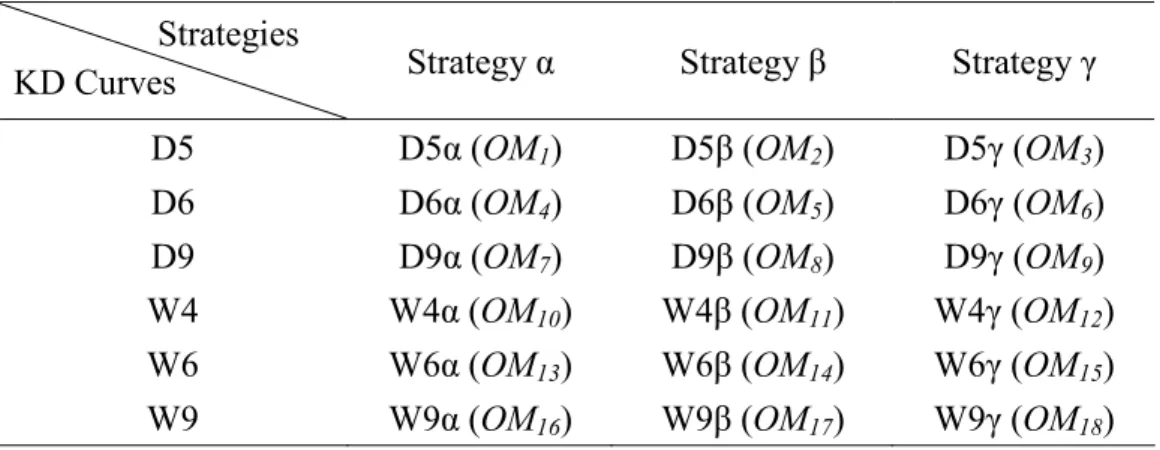
(17) Stock Price. ht Ft. Stτ. St. Stock Price. Ct Ft. Ct-1. Ct-1. Ct-1 Ft. Kt-1<Dt-1. Buy Signal. Dt-1 Kt-1. Start of Periodt. Buy Action. Kt>Dt. Kt-1>Dt-1. Kt-1. Kt Dt-1. Dt. End of Periodt. Start of Periodt. Fig.7. Strategy γ, Situation γ1, Kt-1<Dt-1 and Ct> Ft. Ct-1. Stτ St Sell Signal. lt Sell Action. Ft Ct. Kt<Dt Dt Kt. End of Periodt. Fig.8. Strategy γ, Situation γ2, Kt-1>Dt-1 and Ct< Ft. 9.

(18) 3. Eighteen stock operation methods under selection. The Raw Stochastic Value (RSV) in equation (1) is obtained by past n periods’ data. We consider six ways to compute RSV. Therefore, stock may operate upon six different types of period numbers. D5: n=5, approximately a week. D6: n=6, generally used by broker/dealer firms. D9: n=9, generally used by stock market. W4: n=4, approximately a month. W6: n=6, generally used by portfolio firms. W9: n=9, generally used by stock market. A period could be a day such as D5, D6, and D9, or could be a week such as W4, W6, and W9. There are eighteen possible stock operation methods (OMs), which are the composite of the six ways to determine KD curves and the three strategies, depicted in Table 2, and denoted in a sequence as OM1 , OM2, …, and OM18.. Table 2 Combinations of KD curves and strategies Strategies KD Curves. Strategy α. Strategy β. Strategy γ. D5. D5α (OM1). D5β (OM2). D5γ (OM3). D6 D9 W4 W6 W9. D6α (OM4) D9α (OM7) W4α (OM10) W6α (OM13) W9α (OM16). D6β (OM5) D9β (OM8) W4β (OM11) W6β (OM14) W9β (OM17). D6γ (OM6) D9γ (OM9) W4γ (OM12) W6γ (OM15) W9γ (OM18). 10.

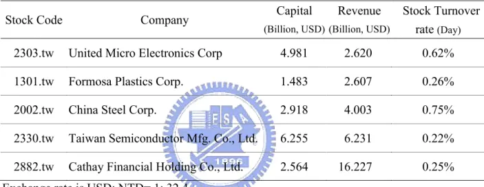
(19) 4. Performance assessment of the eighteen OMs. We selected five major stocks in Taiwan for simulation, as shown in Table 4. These are leading companies in electronics, plastics, steels, and financial industries. The historic data in the periods between January 2nd 2001 to December 31st 2004, 991 days or 206 weeks are collected. The profiles of the five stocks studied in this research are listed in Table 3.. Table 3 Profiles of five major stocks in 2003 Stock Code. Capital. Company. Revenue. (Billion, USD) (Billion, USD). Stock Turnover rate (Day). 2303.tw. United Micro Electronics Corp. 4.981. 2.620. 0.62%. 1301.tw. Formosa Plastics Corp.. 1.483. 2.607. 0.26%. 2002.tw. China Steel Corp.. 2.918. 4.003. 0.75%. 2330.tw. Taiwan Semiconductor Mfg. Co., Ltd.. 6.255. 6.231. 0.22%. 2882.tw. Cathay Financial Holding Co., Ltd.. 2.564. 16.227. 0.25%. Exchange rate is USD: NTD= 1: 32.4. There are several given conditions for the eighteen stock operation methods. The methods are only applied on the Buy-first, Sell-later situation. Margin, short, and day-trade are permitted, and the margin fee and short fee are not considered. The service charge fee for the broker is 0.1425% and the stock trading tax is 0.3%. Trading unit is defined as per share. Buying or selling is activated, without considering limit up, limit down, and trading volume. Data Envelopment Analysis (DEA) [5] [6] [7] was first introduced by Charnes, Cooper, and Rhodes (1978). The efficiency frontier is obtained by adopting non-predetermined production function rather than often used “predetermined production function.” Based on the efficient frontier, technical efficiency and price efficiency of units are assessed. DEA borrows. 11.

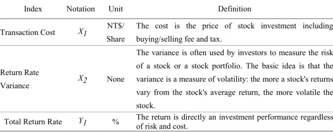
(20) the envelopment concept, setting production frontier in order to distinguish efficient and inefficient Decision Making Units (DMUs). In order to commemorate their contribution, this model is named after the three with the short name of CCR model. This model is based on the linear programming technique with the frontier formed by the “best possibilities” of all possibilities. The DEA model projects the assessment unit input and output items into geometric space, establishing the frontier. The DEA model regards those which fall into the frontier as the most efficient combinations of input and output and therefore assigns them the efficiency index of 1. For those units that fail to fall into the frontier, a relative efficiency index is assigned based on a specific point, which ranges between 0 and 1. As a result, the DEA is capable of resolving controversies caused by assigned weights. A more objective approach is therefore used to assess efficiencies among DMUs.. 4.1 Performance indices Performance indices are critical for analysis of strategy efficiency for stock trading. A set of effective performance indices can truly reflect stock trading features. Table 4 shows the clear definition and description for each index and the feasibility of efficiency analysis.. Table 4 The Indices Index Transaction Cost. Notation X1. Unit. Definition. NT$/. The cost is the price of stock investment including. Share. buying/selling fee and tax. The variance is often used by investors to measure the risk. Return Rate Variance. Total Return Rate. of a stock or a stock portfolio. The basic idea is that the X2. None. variance is a measure of volatility: the more a stock's returns vary from the stock's average return, the more volatile the. Y1. %. stock. The return is directly an investment performance regardless of risk and cost.. 12.

(21) In order to truly simulate the real stock operation, 0.1425% of fee was charged as part of the initial cost. When the stock was sold at the end, 0.1425% of fee and 0.3% of tax were charged. If OMj operates to the set of historic data, mj buying-selling transactions occur. For the ith transaction, the buying and selling price is denoted as Pijbuy and Pijsell , respectively. Data for OMj on the three indices X1, X2, and Y1, are x1j, x2j and y1j, respectively, and can be obtained as follows: The trading cost of the i-th transaction Aij is computed as following Aij = Pijbuy × 0.1425% + Pijsell × (0.1425% + 0.3%). (10). mj. x1 j = ∑ Aij. (11). i =1. The return of OMj at the i-th buying-selling transaction is: Rij =. Pijsell − Pijbuy − Aij Pijbuy × ( 1 + 0.1425%). × 100%. (12). The average return of each buying-selling transaction is:. µj =. R1 j + R2 j + ... + Rm j j. (13). mj. The return rate variance of each buying-selling transaction is: mj. ∑ ( Rij - µ j ) 2 x2 j = Var ( Rij ) =. i =1. (14). mj. The return of OMj at each buying-selling transaction is: mj. y1 j = ∑ Rij. (15). i =1. 13.

(22) 4.2 Assessing efficiency of OMk We define the OMk efficiency score in equation (16). hk is equal to the weighted to-bemaximized indices, X1~X2, divided by the weighted value of to-be-minimized indices Y1 . hk =. y 1k u 1 − u 0 x1 k v1 + x 2 k v 2. (16). The indices in the denominator, Aij and Var(Rij) are called to-be-minimized indices since the efficiency score will be greater as they become smaller in the above equation. On the contrary, when the index of the numerator, Rij get greater, the efficiency score will be greater. This is the so-called to-be-maximized index. However, the above-said weights (v1, v2, u1) will determine efficiency score so controversies arise as to the values accorded to the weights. The following fractional programming model (FPk) is employed to measure the relative efficiency of OMk among the eighteen OMs. The eighteen OMs take turns being the object, represented by OMk. (BCC_I_FPk). (17). Max hk =. st. y 1k u 1 − u 0 x1 k v 1 + x 2 k v 2. y1 j u 1 − u0 x1 j v1 + x 2 j v 2. ≤1. j = 1,2,...,18. u1 ≥ ε > 0 v1 , v 2 ≥ ε > 0 ,. ε is an non-Archimedean small number. The objective function is to determine the optimal decision variables v1 , v 2 , u 1 so that the efficiency score hk is maximized. Each of the eighteen constraints used to limit the efficiency score of OMj is no more than 1. Since a solution cannot be obtained under the FPk. 14.

(23) model, mathematics conversion is borrowed to obtain standard linear programming. The conversion is below: (BCC_I_LPk). (18). min hk = y1k u1 − u0 st. x 1 k v1 + x 2 k v 2 = 1 − x1 j v 1 − x 2 j v 2 + y 1 j u 1 − u 0 ≤ 0. u 1 , v1 , v 2 ≥ ε > 0,. j = 1,2,...,18. ε : non - Archimedean small number. Further convert LPk into dual type, as follows: (BCC_I_DLPk). (19). θ k + ε ( s1− + s 2− + s1+ ). max. 18. y1k − ∑ y 1 j λ j + s1+ = 0. st. j =1. 18. ∑x j =1. ij. λ j + si− = θ k xik. 18. ∑λ j =1. j. =1. λ j ≥ 0, θk. i = 1,2. j = 1,2,...,18. free in sign ,. s1− , s 2− , s1+ ≥ 0. Since ε is very small, it is difficult to assign a value to it. Given that inappropriate assignment will lead to errors, a two-stage calculation is required to obtain the solution. First Stage to obtain solution for θk* (BCC_I_DLPk -I) θk* = max. (20). θk. 15.

(24) 18. st. y 1k − ∑ y 1 j λ j ≤ 0 j =1. 18. ∑x j =1. ij. λ j ≤ θ k xik. 18. ∑λ j =1. j. =1. λ j ≥ 0,. θk. i = 1,2. j = 1,2,...,18. free in sign. Second Stage to obtain solution for s1-*, s2-*, s1+* (BCC_I_DLPk -II) max. (21) s1+ + s1− + s 2−. 18. st. ∑y j =1. 1j. 18. ∑x j =1. ij. λ j − s1+ = y 1k. λ j + si− = θ k∗ xik. 18. ∑λ j =1. λ j ≥ 0,. j. i = 1,2. =1 j = 1,2,...,18. s1− , s 2− , s1+ ≥ 0. The best weight when θk*, s1-*, s2-*, s1+* are obtained by the best solution of DLPk, the * * * * best solutions for hk , v1 , v2 , u1 are obtained. The efficiency of OMk is as follows:. hk* =. y 1 k u *1 − u 0*. (22). x 1 k v *1 + x 2 k v 2*. When denominator is 1, then hk* = y 1k u 1* − u 0*. 16.

(25) 4.3 Computation of super-efficiency The super-efficiency introduced by Andersen & Petersen (1993) [8] is used to compute the efficiencies of DMUs. If the object DMU, DMUk, is an efficient unit, its super-efficiency can be measured. (AP-BCC_I_DLPk -I). θk. θ k* = max st. (23). 18. ∑y. y 1k −. j =1, j ≠ k. 18. ∑x λ. j =1, j ≠ k. ij. j. 18. ∑λ. j =1, j ≠ k. λj ≤ 0. ≤ θ k xik. i = 1,2. =1. j. λ j ≥ 0,. θk. 1j. j = 1,2,...,18 , j ≠ k. free in sign. The second phase is as follows: (AP-BCC_I_DLPk -II) max. s1+ + s1− + s 2− 18. st. (24). ∑y. j =1, j ≠ k. 1j. λ j − s1+ = y1k. 18. ∑x λ. j =1, j ≠ k. ij. 18. ∑λ. j =1, j ≠ k. λ j ≥ 0,. j. j. + s i− = θ k∗ xik. i = 1,2. =1 j = 1,2,...,18 , j ≠ k. 17.

(26) s1− , s 2− , s1+ ≥ 0. Certain efficient DMUs may result in an infeasible solution. We further employed Yao Chen method [9][10] to obtain appropriate super-efficiency. If the DMUk is infeasible in models (23), we compute the projection point of each inefficient DMU on the efficient frontier. The projection point is denoted as yˆ rk . yˆ rk = θ k* yrk . The following model computes the efficient DMU projection point on the frontier. ~. ~. θ k* = min θ k n. s.t.. ∑λ x. j ij. j =1 j≠k n. ∑ λ yˆ j. j =1 j ≠k n. ∑λ j =1 j ≠k. j. rj. (25). ~ ≤ θ k xik , i = 1,2,..., m, ≥ yˆ rk = yrk , r = 1,2,..., s,. = 1,. λ j ≥ 0,. j ≠ k.. The super-efficiency of DMUk, φk is obtained according to the following situations.. θk ~* φk = θk 1,  *. if model (23) is feasible if model (23) is infeasible and model (25) is feasible if model (25) is infeasible. 18.

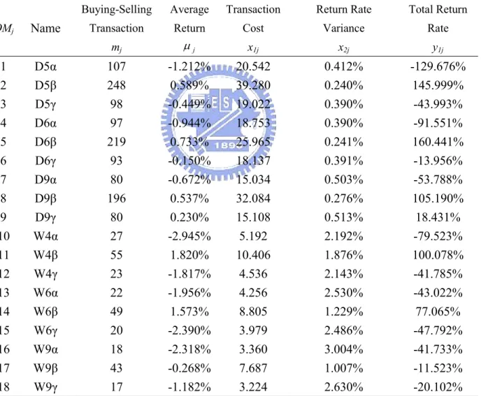
(27) 5. Computation and results. 5.1 The computation of UMC UMC (2303.tw) is a popular high-tech stock with heavy trading volume and also favored by individual investors and broker/dealer firms. The three indices data of the eighteen OMs are depicted in Table 5.. Table 5 Performance data of the eighteen OMs of UMC (2303.tw) OMj. 1 2 3 4 5 6 7 8 9 10 11 12 13 14 15 16 17 18. Name D5α D5β D5γ D6α D6β D6γ D9α D9β D9γ W4α W4β W4γ W6α W6β W6γ W9α W9β W9γ. Buying-Selling. Average. Transaction. Return Rate. Total Return. Transaction. Return. Cost. Variance. Rate. mj. µj. x1j. x2j. y1j. 107 248 98 97 219 93 80 196 80 27 55 23 22 49 20 18 43 17. -1.212% 0.589% -0.449% -0.944% 0.733% -0.150% -0.672% 0.537% 0.230% -2.945% 1.820% -1.817% -1.956% 1.573% -2.390% -2.318% -0.268% -1.182%. 20.542 39.280 19.022 18.753 25.965 18.137 15.034 32.084 15.108 5.192 10.406 4.536 4.256 8.805 3.979 3.360 7.687 3.224. 0.412% 0.240% 0.390% 0.390% 0.241% 0.391% 0.503% 0.276% 0.513% 2.192% 1.876% 2.143% 2.530% 1.229% 2.486% 3.004% 1.007% 2.630%. -129.676% 145.999% -43.993% -91.551% 160.441% -13.956% -53.788% 105.190% 18.431% -79.523% 100.078% -41.785% -43.022% 77.065% -47.792% -41.733% -11.523% -20.102%. The eighteen OM data consisting of trading fee, return rate variance, and total return rate listed in table 5, was analyzed with DEA analysis. The results are φk , ν 1∗ , ν 2∗ , u 0* , and u1* .. 19.

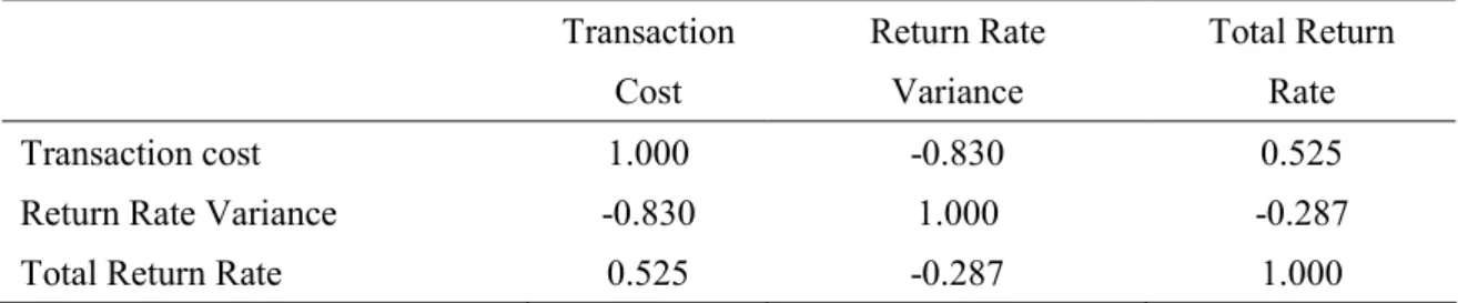
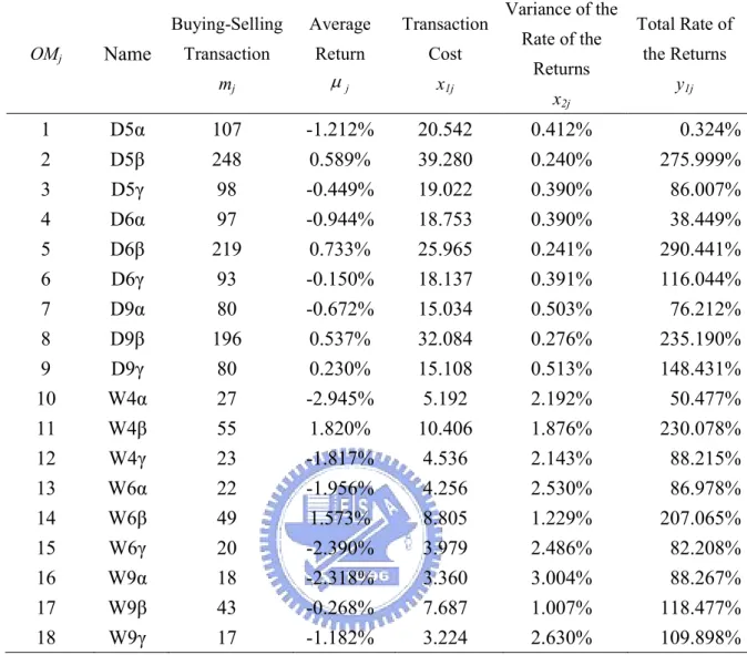
(28) Table 6 results show a weak relationship between indices. One substitutes Aij into equation (12) would find Rij is a function of Pbuy and Psell. We could not directly tell the correlation between Aij and Rij. From equations (13) and (14), we can tell the negative correlation between Aij and Var(Rij). This strongly suggests that index selection is proper and reasonable.. Table 6 Correlation between indices Transaction. Return Rate. Total Return. Cost. Variance. Rate. Transaction cost. 1.000. -0.830. 0.525. Return Rate Variance. -0.830. 1.000. -0.287. Total Return Rate. 0.525. -0.287. 1.000. Negative data is evident in column y1j in Table 5. We transform the data to positive by adding 130% to each value. The resulting data is depicted in Table 7.. 20.

(29) Table 7 Transformed data of UMC. OMj. Name. Buying-Selling. Average. Transaction. Transaction. Return. Cost. mj. µj. x1j. Variance of the Rate of the Returns. x2j. Total Rate of the Returns. y1j. 1. D5α. 107. -1.212%. 20.542. 0.412%. 0.324%. 2 3 4 5 6 7 8 9 10 11 12 13 14 15 16 17 18. D5β D5γ D6α D6β D6γ D9α D9β D9γ W4α W4β W4γ W6α W6β W6γ W9α W9β W9γ. 248 98 97 219 93 80 196 80 27 55 23 22 49 20 18 43 17. 0.589% -0.449% -0.944% 0.733% -0.150% -0.672% 0.537% 0.230% -2.945% 1.820% -1.817% -1.956% 1.573% -2.390% -2.318% -0.268% -1.182%. 39.280 19.022 18.753 25.965 18.137 15.034 32.084 15.108 5.192 10.406 4.536 4.256 8.805 3.979 3.360 7.687 3.224. 0.240% 0.390% 0.390% 0.241% 0.391% 0.503% 0.276% 0.513% 2.192% 1.876% 2.143% 2.530% 1.229% 2.486% 3.004% 1.007% 2.630%. 275.999% 86.007% 38.449% 290.441% 116.044% 76.212% 235.190% 148.431% 50.477% 230.078% 88.215% 86.978% 207.065% 82.208% 88.267% 118.477% 109.898%. By implementing models (23) or (25), the following efficiencies are obtained, as in Table 8.. 21.

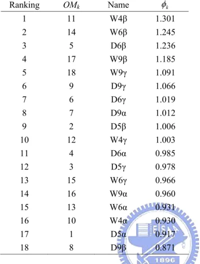
(30) Table 8 Efficiency of eighteen OMs of UMC OMk. Name. φk. 1. D5α. 0.917. 17. 2 3 4 5 6 7 8 9 10 11 12 13 14 15 16 17 18. D5β D5γ D6α D6β D6γ D9α D9β D9γ W4α W4β W4γ W6α W6β W6γ W9α W9β W9γ. 1.006 0.978 0.985 1.236 1.019 1.012 0.871 1.066 0.930 1.301 1.003 0.931 1.245 0.966 0.960 1.185 1.091. 9 12 11 3 7 8 18 6 16 1 10 15 2 13 14 4 5. Ranking. Efficiencies sorted to ranking order.. 22.

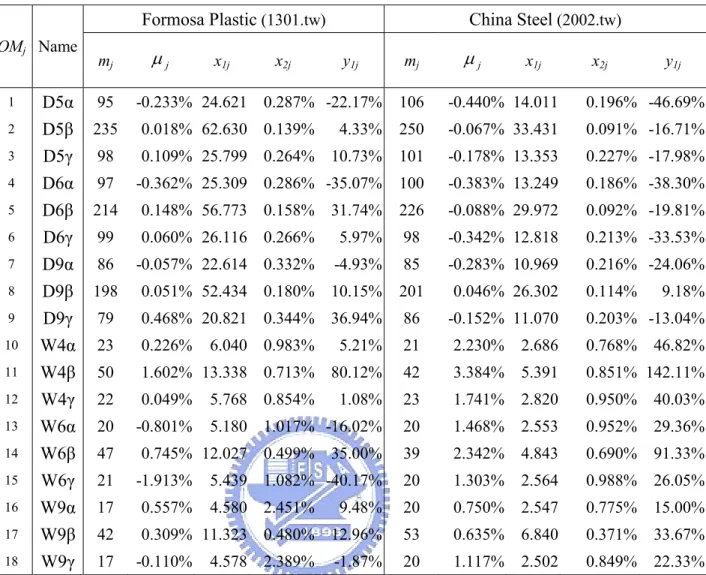
(31) Table 9 Efficiency ranking of eighteen OMs of UMC Ranking. OMk. Name. φk. 1. 11. W4β. 1.301. 2 3 4 5 6 7 8 9 10 11 12 13 14 15 16 17 18. 14 5 17 18 9 6 7 2 12 4 3 15 16 13 10 1 8. W6β D6β W9β W9γ D9γ D6γ D9α D5β W4γ D6α D5γ W6γ W9α W6α W4α D5α D9β. 1.245 1.236 1.185 1.091 1.066 1.019 1.012 1.006 1.003 0.985 0.978 0.966 0.960 0.931 0.930 0.917 0.871. From the above result, we know W4β is ranked to 1. Its efficiency is superior to other OMs. It exhibited excellent control in input or outstanding performance in output.. 5.2 Original data for the other four stocks We also collected data for the other four major stocks in Taiwan. Appendix Tables T1~T18 depict some of the original data for the five stocks operated by Strategies α, β, and γ. Following the same process as used for UMC stock, values of performance indices for the four stocks are obtained, as depicted in Tables 10 and 11. There are negative values in the columns of y1j. We transform those to positive. The resulting data is depicted in Tables 12 and 13.. 23.

(32) Table 10 Formosa Plastic and China Steel Stock Data Formosa Plastic (1301.tw) OMj Name 1 2 3 4 5 6 7 8 9 10 11 12 13 14 15 16 17 18. mj. D5α 95 D5β 235 D5γ 98 D6α 97 D6β 214 D6γ 99 D9α 86 D9β 198 D9γ 79 W4α 23 W4β 50 W4γ 22 W6α 20 W6β 47 W6γ 21 W9α 17 W9β 42 W9γ 17. µj. x1j. China Steel (2002.tw). x2j. y1j. -0.233% 24.621 0.287% -22.17%. mj. µj. x1j. x2j. y1j. 106. -0.440% 14.011. 0.196% -46.69%. 4.33%. 250. -0.067% 33.431. 0.091% -16.71%. 0.109% 25.799 0.264% 10.73%. 101. -0.178% 13.353. 0.227% -17.98%. -0.362% 25.309 0.286% -35.07%. 100. -0.383% 13.249. 0.186% -38.30%. 0.148% 56.773 0.158% 31.74%. 226. -0.088% 29.972. 0.092% -19.81%. 0.060% 26.116 0.266%. 5.97%. 98. -0.342% 12.818. 0.213% -33.53%. -0.057% 22.614 0.332%. -4.93%. 85. -0.283% 10.969. 0.216% -24.06%. 0.051% 52.434 0.180% 10.15%. 201. 0.046% 26.302. 0.468% 20.821 0.344% 36.94%. 86. -0.152% 11.070. 0.226%. 5.21%. 21. 2.230%. 2.686. 0.768%. 1.602% 13.338 0.713% 80.12%. 42. 3.384%. 5.391. 0.851% 142.11%. 0.049%. 1.08%. 23. 1.741%. 2.820. 0.950%. 40.03%. 5.180 1.017% -16.02%. 20. 1.468%. 2.553. 0.952%. 29.36%. 0.745% 12.027 0.499% 35.00%. 39. 2.342%. 4.843. 0.690%. 91.33%. 5.439 1.082% -40.17%. 20. 1.303%. 2.564. 0.988%. 26.05%. 4.580 2.451%. 9.48%. 20. 0.750%. 2.547. 0.775%. 15.00%. 0.309% 11.323 0.480% 12.96%. 53. 0.635%. 6.840. 0.371%. 33.67%. 20. 1.117%. 2.502. 0.849%. 22.33%. 0.018% 62.630 0.139%. -0.801% -1.913% 0.557% -0.110%. 6.040 0.983% 5.768 0.854%. 4.578 2.389%. -1.87%. 24. 0.114%. 9.18%. 0.203% -13.04% 46.82%.

(33) Table 11 Taiwan Semiconductor Manufacturing Company (TSMC) and Cathay Financial Holding Company (CFHC) Stock Data TSMC (2330.tw). OMj Name 1 2 3 4 5 6 7 8 9 10 11 12 13 14 15 16 17 18. D5α D5β D5γ D6α D6β D6γ D9α D9β D9γ W4α W4β W4γ W6α W6β W6γ W9α W9β W9γ. mj. µj. x1j. CFHC (2882.tw). x2j. y1j. mj. µj. x1j. x2j. y1j. 100 -0.717% 36.712 0.426% -71.71%. 109 -0.563% 31.533. 0.252% -61.41%. 185 0.869% 67.954 0.257% 160.71%. 237 -0.033% 68.997. 0.164%. 98 0.273% 36.349 0.393% 26.75%. 100 -0.177% 29.090. 0.325% -17.72%. 94 -0.711% 34.509 0.467% -66.84%. 103 -0.507% 29.872. 0.254% -52.23%. 177 0.809% 65.406 0.287% 143.11%. 224 -0.137% 64.634. 0.159% -30.59%. 90 0.321% 33.175 0.437% 28.91%. 98 -0.241% 28.520. 0.301% -23.61%. 84 -0.765% 30.717 0.506% -64.28%. 91 -0.127% 26.373. 0.259% -11.55%. 174 0.421% 64.861 0.313% 73.26%. 214 -0.119% 61.772. 0.152% -25.42%. 82 0.266% 30.220 0.544% 21.77%. 86 0.099% 25.001. 0.313%. 29 -1.432% 11.442 1.269% -41.53%. 24 -0.846%. 6.839. 0.798% -20.30%. 57 0.870% 22.274 0.607% 49.62%. 43 1.438% 12.591. 0.483% 61.85%. 26 -1.484% 10.216 1.535% -38.59%. 23 -0.020%. 6.599. 0.790%. 21 0.191%. 21 -2.061%. 5.927. 0.920% -43.28%. 47 1.280% 17.624 0.985% 60.17%. 41 0.762% 11.700. 0.659% 31.23%. 20 -1.607%. 7.685 2.396% -32.14%. 21 -0.775%. 6.006. 0.959% -16.28%. 20 -3.806%. 7.298 2.747% -76.13%. 18 0.811%. 5.136. 1.299% 14.59%. 41 0.252% 15.275 1.318% 10.33%. 40 0.546% 10.662. 0.439% 21.85%. 20 -1.932%. 18 0.484%. 1.061%. 7.994 2.228%. 4.01%. 7.307 2.510% -38.64%. 25. 5.141. -7.73%. 8.51%. -0.46%. 8.72%.

(34) Table 12 Formosa Plastic and China Steel Transformed Stock Data Formosa Plastic (1301.tw) OMj Name 1 2 3 4 5 6 7 8 9 10 11 12 13 14 15 16 17 18. mj. D5α 95 D5β 235 D5γ 98 D6α 97 D6β 214 D6γ 99 D9α 86 D9β 198 D9γ 79 W4α 23 W4β 50 W4γ 22 W6α 20 W6β 47 W6γ 21 W9α 17 W9β 42 W9γ 17. µj. x1j. x2j. China Steel (2002.tw) y1j. mj. µj. x1j. x2j. y1j 0.31%. -0.233% 24.621 0.287% 18.83%. 106. -0.440% 14.011. 0.196%. 0.018% 62.630 0.139% 45.33%. 250. -0.067% 33.431. 0.091% 30.29%. 0.109% 25.799 0.264% 51.73%. 101. -0.178% 13.353. 0.227% 29.02%. 5.93%. 100. -0.383% 13.249. 0.186%. 0.148% 56.773 0.158% 72.74%. 226. -0.088% 29.972. 0.092% 27.19%. 0.060% 26.116 0.266% 46.97%. 98. -0.342% 12.818. 0.213% 13.47%. -0.057% 22.614 0.332% 36.07%. 85. -0.283% 10.969. 0.216% 22.94%. 0.051% 52.434 0.180% 51.15%. 201. 0.046% 26.302. 0.114% 56.18%. 0.468% 20.821 0.344% 77.94%. 86. -0.152% 11.070. 0.203% 33.96%. 0.226%. 6.040 0.983% 46.21%. 21. 2.230%. 2.686. 0.768% 93.82%. 1.602% 13.338 0.713% 121.12%. 42. 3.384%. 5.391. 0.851% 189.11%. 0.049%. 5.768 0.854% 42.08%. 23. 1.741%. 2.820. 0.950% 87.03%. -0.801%. 5.180 1.017% 24.98%. 20. 1.468%. 2.553. 0.952% 76.36%. 0.745% 12.027 0.499% 76.00%. 39. 2.342%. 4.843. 0.690% 138.33%. 0.83%. 20. 1.303%. 2.564. 0.988% 73.05%. 4.580 2.451% 50.48%. 20. 0.750%. 2.547. 0.775% 62.00%. 0.309% 11.323 0.480% 53.96%. 53. 0.635%. 6.840. 0.371% 80.67%. 20. 1.117%. 2.502. 0.849% 69.33%. -0.362% 25.309 0.286%. -1.913% 0.557% -0.110%. 5.439 1.082%. 4.578 2.389% 39.13%. 26. 8.70%.

(35) Table 13 Taiwan Semiconductor Manufacturing Company (TSMC) and Cathay Financial Holding Company (CFHC) Transformed Stock Data TSMC (2330.tw). OMj Name 1 2 3 4 5 6 7 8 9 10 11 12 13 14 15 16 17 18. D5α D5β D5γ D6α D6β D6γ D9α D9β D9γ W4α W4β W4γ W6α W6β W6γ W9α W9β W9γ. mj. µj. x1j. CFHC (2882.tw). x2j. y1j. 100 -0.717% 36.712 0.426%. mj. µj. x1j. x2j. y1j 0.59%. 5.29%. 109 -0.563% 31.533. 0.252%. 185 0.869% 67.954 0.257% 237.71%. 237 -0.033% 68.997. 0.164% 54.27%. 98 0.273% 36.349 0.393% 103.75%. 100 -0.177% 29.090. 0.325% 44.28%. 94 -0.711% 34.509 0.467% 10.16%. 103 -0.507% 29.872. 0.254%. 177 0.809% 65.406 0.287% 220.11%. 224 -0.137% 64.634. 0.159% 31.41%. 90 0.321% 33.175 0.437% 105.91%. 98 -0.241% 28.520. 0.301% 38.39%. 84 -0.765% 30.717 0.506% 12.72%. 91 -0.127% 26.373. 0.259% 50.45%. 174 0.421% 64.861 0.313% 150.26%. 214 -0.119% 61.772. 0.152% 36.58%. 82 0.266% 30.220 0.544% 98.77%. 86 0.099% 25.001. 0.313% 70.51%. 29 -1.432% 11.442 1.269% 35.47%. 24 -0.846%. 6.839. 0.798% 41.70%. 57 0.870% 22.274 0.607% 126.62%. 43 1.438% 12.591. 0.483% 123.85%. 26 -1.484% 10.216 1.535% 38.41%. 23 -0.020%. 6.599. 0.790% 61.54%. 21 0.191%. 21 -2.061%. 5.927. 0.920% 18.72%. 47 1.280% 17.624 0.985% 137.17%. 41 0.762% 11.700. 0.659% 93.23%. 20 -1.607%. 7.685 2.396% 44.86%. 21 -0.775%. 6.006. 0.959% 45.72%. 20 -3.806%. 7.298 2.747%. 18 0.811%. 5.136. 1.299% 76.59%. 41 0.252% 15.275 1.318% 87.33%. 40 0.546% 10.662. 0.439% 83.85%. 20 -1.932%. 18 0.484%. 1.061% 70.72%. 7.994 2.228% 81.01%. 0.87%. 7.307 2.510% 38.36%. 27. 5.141. 9.77%.

(36) 5.3 Eighteen OMs Performance for the five stocks Performance rankings of the eighteen OMs for the five stocks are summarized in Table 14.. Table 14 Performance rankings of the eighteen OMs for the five stocks Ranking. 2303.tw. 1301.tw. 2002.tw. 2330.tw. 2882.tw. 1. W4β (1.301). W4β (1.561). D9β (1.891). W6α (1.257). W4β (1.366). 2 3 4 5 6 7 8 9 10 11 12 13 14 15 16 17 18. W6β (1.245) D6β (1.236) W9β (1.185) W9γ (1.091) D9γ (1.066) D6γ (1.019) D9α (1.012) D5β (1.006) W4γ (1.003) D6α (0.985) D5γ (0.978) W6γ (0.966) W9α (0.960) W6α (0.931) W4α (0.930) D5α (0.917) D9β (0.871). W9α (1.264) D5β (1.137) D6β (1.134) W4γ (1.102) W6β (1.070) W6α (1.053) W9β (1.053) D9γ (1.038) D5γ (1.009) W9γ (1.005) W4α (0.994) D6γ (0.993) D5α (0.992) D9β (0.982) D6α (0.979) D9α (0.970) W6γ (0.951). W9β (1.174) W4α (1.123) D6β (1.054) D9γ (1.038) W6β (1.037) D5β (1.035) W9α (1.029) W9γ (1.019) D6α (1.014) W6α (1.000) W6γ (0.987) D9α (0.985) D5α (0.948) W4γ (0.934) D6γ (0.923) W4β (0.898) D5γ (0.874). W6β (1.223) W4β (1.146) D5β (1.118) W4α (1.080) D5γ (1.046) W9γ (1.031) W4γ (1.017) D6γ (1.005) W9α (1.001) W6γ (0.993) D6β (0.971) D9α (0.969) D5α (0.959) D6α (0.949) D9γ (0.939) D9β (0.927) W9β (0.921). D5β (1.200) W9α (1.159) W9β (1.144) W9γ (1.067) D9α (1.056) D9β (1.049) W4γ (1.024) D9γ (1.001) W6α (0.997) D6α (0.983) W4α (0.979) D5α (0.974) W6γ (0.972) D6β (0.955) D6γ (0.894) W6β (0.867) D5γ (0.853). The eighteen OMs are ordered according to their weighted sum. Rank 1 to Rank 18 are weighted by 18 to 1, respectively. As shown in Table 15, we further divide the eighteen OMs into three parts. The first six OMs, ranking 1~6, are W4β, D5β, W6β, W9β, W9α, and W9γ. We summarize that the combinations of strategy β and n-week KD are outperformed than others. Oppositely, the last six OMs, ranking 13~18, D9β, D6γ, D6α, D5γ, W6γ, and D5α, the combinations of strategy α and n-day KD, performed poorly.. 28.

(37) Table 15 Overall ranking of the OMs in the five stocks Ranking OM W4β. 3 1. 2. 3. 4. 1. W6β. 2. W9β. 1. W9α. 1. 1. 1. 9. 10 11 12 13 14 15 16 17 18. 1. 2. 1. 2. 1. 1 1. 1. 1 1. 1 1. 1 1. 2. 1. 1. 1. D9γ. 1. W4γ. 1. W4α. 8. 1. 2. D6β. 7. 1. W9γ. 1. 1. 1. 1. 2 2. 1 1. 1 2. 1 1. 1. 1 2. 1. 1. D6γ. 1. 1. 1. D6α D5γ. 1. 1. 1. D9α D9β. 6. 1. D5β. W6α. 5. 1 1. 1. W6γ. 1. 1. 1 1. D5α. 1. 2 1. 1. 1. 3. 1 1. 5.4 Tick size impact analysis Tick size ∆ varies corresponding to the stock prices, p. [11] ∆=NT$0.01 if p < NT$5; ∆=NT$0.05 if NT$5 ≤ p<NT$15; ∆=NT$0.1 if NT$15 ≤ p <NT$50; ∆=NT$0.5 if NT$50 ≤ p <NT$150; ∆=NT$1.0 if NT$150 ≤ p <NT$1000; ∆=NT$5.0 if NT$1000 ≤ p. Given a tick size, let pL and pU be the lower bound and the upper bound of stock prices. The average impact of the tick size is computed by the following equation.. 29. 1. 2. 2. 1. 1.

(38) I= [2*∆/(pL + pU)]*100% The following table depicts the average tick size impact on various stock prices. In our simulation of stock 2330.tw under operation methods W6α, W6β, and W4β, trading frequencies are also listed.. Table 16 Tick size impact of 2330.tw Price range pL. Counts of trading frequencies of 2330.tw. Tick size. pU. (△). W6α. W6β. Count Count. W4β. Difference with W6α. Count. Tick size impact (I). Difference with W6α. 40. 45. 0.1. 3. 6. -0.71%. 6. -0.71%. 0.24%. 45. 50. 0.1. 2. 10. -1.68%. 7. -1.05%. 0.21%. 50. 55. 0.5. 2. 1. 0.95%. 5. -2.86%. 0.95%. 55. 60. 0.5. 3. 7. -3.48%. 5. -1.74%. 0.87%. 60. 65. 0.5. 3. 3. 0.00%. 6. -2.40%. 0.80%. 65. 70. 0.5. 1. 7. -4.44%. 8. -5.19%. 0.74%. 70. 75. 0.5. 0. 0. 0.00%. 2. -1.38%. 0.69%. 75. 80. 0.5. 1. 0. 0.65%. 0. 0.65%. 0.65%. 80. 85. 0.5. 1. 2. -0.61%. 4. -1.82%. 0.61%. 85. 90. 0.5. 4. 5. -0.57%. 6. -1.14%. 0.57%. 90. 95. 0.5. 1. 5. -2.16%. 6. -2.70%. 0.54%. 95 100. 0.5. 0. 0.00%. 2. -1.03%. 0.51%. 100 110. 0.5. 1. -0.48%. 47. -12.53%. Total. 21. 0.48% 57. -21.36%. We also obtain tick size impact, -12.53% and -21.36%, from the difference between W6β and W6α, and between W4β and W6α. That means the overall performance of 2330.tw is heavily impacted by tick size. This is one of the reasons that strategy α outperforms β as shown in Table 14.. 30.

(39) 6. Conclusions. We proposed two new strategies in this research, aside from the conventional stock buying-selling strategy and KD curves. We also considered the performance of the three strategies under six different period lengths. Combining of period lengths with buying-selling strategies, created eighteen stock operation methods to select. We simulated five major stocks in Taiwan and accessed the performance of the eighteen operation methods. The indices selection is a key point. Other factors that may influence the stock market include politics, economics, and natural or man-made calamities (ex. earthquake, SARS, war, etc.). Transaction cost, risk of investment, and net return from trading are used as performance indices in this research. The performance index should not be limited. Depending on the interest, employment performance indices will lead to different results. Obviously, each stock has its own market characteristics. One stock may be active and have a wider variation range than others. The eighteen OMs perform differently in various stocks. Reaching a firm conclusion for ranking the eighteen OMs to all the stocks may be difficult. We recommend that portfolio managers or individual investors buy/sell a stock using the OM with the highest performance based on its historical data. Using Strategy β with KD curves will overreact on buying/selling, and the increased transaction cost will harm performance. On the other hand, using Strategy γ with KD curves may miss good timing for buying/selling. Conventional KD indicators are less reliable. To use a particular analysis method for a specific stock, the investor could search for optimal parameter settings for the method, such as reviewing period length and operation strategy.. 31.

(40) References [1] George C. Lane, Trading Strategies Futures Symposium International, 1984. [2] George C. Lane, Technical Analysis of Stocks and Commodities magazine, May/June, pp.87-90, 1984. [3] Welles, Wilder, New Concepts in Technical Trading Systems, Trend Research, New York, 1978. [4] Richard Donchian & J. M. Hurst, http://www.turtletrader.com/trader-donchian.html [5] Emmanuel Thanassoulis, Introduction to the Theory and Application of Data Envelopment Analysis, Kluwer Academic Publishers, Boston, 2001. [6] William W. Cooper, Lawrence M. Seiford, Kaoru Tone, Data Envelopment Analysis: A Comprehensive Text with Models, Applications, References and DEA-Solver Software, Kluwer Academic Publishers, Boston, 2000. [7] Fuh-Hwa Liu, “The course material of Performance Evaluation Technology, DEA”, Department of Industrial Engineering and Management, National Chiao Tung University, Taiwan, 2003. [8] P. Andersen, and N. Petersen, “A Procedure for Ranking Efficient Units in Data Envelopment Analysis”, Management Science, 39, pp. 1261–1264, 1993. [9] Yao Chen, “Ranking efficient units in DEA”, Omega, 32, pp. 213 – 219, 2004. [10] Yao Chen, “Measuring super-efficiency in DEA in the presence of infeasibility”, European Journal of Operational Research, 161, pp. 545–551, 2005. [11] Taiwan Stock Exchange Corporation, “Trading Mechanism - Tick Size”, 2005. http://www.tse.com.tw/en/products/trading_rules/mechanism02.php. 32.

(41) Appendix T1: The abstract of calculation process for 2303 strategy D5α No 1 2 3 4 5 6 7 8 9 10 11 12 13 14 15. Date 2001/01/02 2001/01/03 2001/01/04 2001/01/05 2001/01/08 2001/01/09 2001/01/10 2001/01/11 2001/01/12 2001/01/15 2001/01/16 2001/01/17 2001/01/18 2001/01/29 2001/01/30. Open High 46.8 50 48 49 50.5 51.5 50.5 53 51 52.5 50.5 53 53 53.5 52.5 53.5 52 53 52 53 53.5 56.5 57.5 59 59.5 59.5 58.5 58.5 54.5 56.5. Low Close 5DHigh 45.8 49.6 50.0 47.5 48.3 50.0 49.6 50.5 51.5 50 52 53.0 50.5 50.5 53.0 50.5 53 53.0 51.5 52 53.5 51 51.5 53.5 51.5 52 53.5 51.5 53 53.5 53.5 56.5 56.5 57 59 59.0 57.5 58.5 59.5 54.5 54.5 59.5 54 56.5 59.5. 5DLow 43.6 45.0 45.8 45.8 45.8 47.5 49.6 50.0 50.5 50.5 51.0 51.0 51.5 51.5 53.5. RSV 93.75 66.00 82.46 86.11 65.28 100.00 61.54 42.86 50.00 83.33 100.00 100.00 87.50 37.50 50.00. K 77.19 73.46 76.46 79.68 74.88 83.25 76.01 64.96 59.97 67.76 78.51 85.67 86.28 70.02 63.35. D KD cross B/S 61.27 45.48 B 65.33 47.45 69.04 48.89 72.59 50.01 73.35 50.86 76.65 50.99 76.44 52.61 S 72.61 53.08 68.40 53.06 68.19 52.57 71.63 54.18 B 76.31 55.61 79.63 56.81 76.43 58.64 S 72.07 58.87. Buy price 46.80. Sell price. 52.5. Return rate. Tax for buying 0.06669. 11.52. 57.50. Tax for selling. 0.2323125. 0.0819375. 54.5. -5.77. 0.2411625. ……………………………………………………………… 978 979 980 981 982 983 984 985 986 987 988 989 990 991. 2004/12/14 2004/12/15 2004/12/16 2004/12/17 2004/12/20 2004/12/21 2004/12/22 2004/12/23 2004/12/24 2004/12/27 2004/12/28 2004/12/29 2004/12/30 2004/12/31. 19.9 20.1 20.3 20.2 19.9 19.9 19.9 19.9 19.9 20 19.8 19.9 20.3 20.3. 20.1 20.4 20.4 20.3 20 20 20.1 20 20 20 20 20.3 20.3 20.5. 19.8 20 20.1 20.1 19.7 19.8 19.9 19.8 19.8 19.8 19.8 19.9 20.1 20.1. 20 20.3 20.2 20.1 19.8 19.8 19.9 19.9 20 19.9 19.8 20.2 20.2 20.5. 20.4 20.4 20.4 20.4 20.4 20.4 20.4 20.3 20.1 20.1 20.1 20.3 20.3 20.5. 19.7 19.7 19.7 19.7 19.7 19.7 19.7 19.7 19.7 19.8 19.8 19.8 19.8 19.8. 42.86 85.71 71.43 57.14 14.29 14.29 28.57 33.33 75.00 33.33 0.00 80.00 80.00 100.00. 30.20 48.70 56.28 56.57 42.47 33.08 31.58 32.16 46.44 42.07 28.05 45.37 56.91 71.27. 33.11 19.97 38.31 19.82 44.30 19.84 48.39 19.92 46.42 20.08 41.97 20.12 38.50 20.07 36.39 19.97 39.74 19.81 40.52 19.91 36.36 19.96 39.36 19.94 45.21 19.91 53.90 19.93 Return -129.68% cost 20.54 Var 0.412%. 33. B 20.30. 0.028927499. S 19.9. -2.54. 0.0880575. B 20.00 S B. 0.0285 19.9. -1.08. 20.30 S 107. 0.0880575 0.028927499. 20.5 107. 0.40 -129.68. 5.03. 0.0907125 15.51.

(42) T2: The abstract of calculation process for 2303 strategy D5β No 1 2 3 4 5 6 7 8 9 10 11 12 13 14 15. Date 2001/01/02 2001/01/03 2001/01/04 2001/01/05 2001/01/08 2001/01/09 2001/01/10 2001/01/11 2001/01/12 2001/01/15 2001/01/16 2001/01/17 2001/01/18 2001/01/29 2001/01/30. Open High 46.8 50 48 49 50.5 51.5 50.5 53 51 52.5 50.5 53 53 53.5 52.5 53.5 52 53 52 53 53.5 56.5 57.5 59 59.5 59.5 58.5 58.5 54.5 56.5. Low Close 5DHigh 45.8 49.6 50.0 47.5 48.3 50.0 49.6 50.5 51.5 50 52 53.0 50.5 50.5 53.0 50.5 53 53.0 51.5 52 53.5 51 51.5 53.5 51.5 52 53.5 51.5 53 53.5 53.5 56.5 56.5 57 59 59.0 57.5 58.5 59.5 54.5 54.5 59.5 54 56.5 59.5. 5DLow 43.6 45.0 45.8 45.8 45.8 47.5 49.6 50.0 50.5 50.5 51.0 51.0 51.5 51.5 53.5. RSV 93.75 66.00 82.46 86.11 65.28 100.00 61.54 42.86 50.00 83.33 100.00 100.00 87.50 37.50 50.00. K 77.19 73.46 76.46 79.68 74.88 83.25 76.01 64.96 59.97 67.76 78.51 85.67 86.28 70.02 63.35. D KD cross B/S 61.27 45.48 B 65.33 47.45 69.04 48.89 72.59 50.01 73.35 50.86 76.65 50.99 SB 76.44 52.61 72.61 53.08 S 68.40 53.06 68.19 52.57 71.63 54.18 B 76.31 55.61 79.63 56.81 76.43 58.64 S 72.07 58.87. Buy price Sell price Return rate Tax for buying Tax for selling 46.80 0.06669. 53.00. 50.50. 7.28. 52.5. -1.52. 53.00. 0.075525. 0.2234625 0.2323125. 0.075525. 56.5. 5.98. 0.2500125. ……………………………………………………………… 978 979 980 981 982 983 984 985 986 987 988 989 990 991. 2004/12/14 2004/12/15 2004/12/16 2004/12/17 2004/12/20 2004/12/21 2004/12/22 2004/12/23 2004/12/24 2004/12/27 2004/12/28 2004/12/29 2004/12/30 2004/12/31. 19.9 20.1 20.3 20.2 19.9 19.9 19.9 19.9 19.9 20 19.8 19.9 20.3 20.3. 20.1 20.4 20.4 20.3 20 20 20.1 20 20 20 20 20.3 20.3 20.5. 19.8 20 20.1 20.1 19.7 19.8 19.9 19.8 19.8 19.8 19.8 19.9 20.1 20.1. 20 20.3 20.2 20.1 19.8 19.8 19.9 19.9 20 19.9 19.8 20.2 20.2 20.5. 20.4 20.4 20.4 20.4 20.4 20.4 20.4 20.3 20.1 20.1 20.1 20.3 20.3 20.5. 19.7 19.7 19.7 19.7 19.7 19.7 19.7 19.7 19.7 19.8 19.8 19.8 19.8 19.8. 42.86 85.71 71.43 57.14 14.29 14.29 28.57 33.33 75.00 33.33 0.00 80.00 80.00 100.00. 30.20 48.70 56.28 56.57 42.47 33.08 31.58 32.16 46.44 42.07 28.05 45.37 56.91 71.27. 33.11 38.31 44.30 48.39 46.42 41.97 38.50 36.39 39.74 40.52 36.36 39.36 45.21 53.90 Return cost Var. 34. 19.97 19.82 B 19.84 19.92 20.08 S 20.12 20.07 19.97 19.81 B 19.91 SB 19.96 S 19.94 B 19.91 19.93 S 146.00% 39.28 0.240%. 20.00. 20.00 19.90. 0.0285. 19.9. -1.08. 19.80 19.9. -1.58 -0.58. 20.00. 248. 0.0880575. 0.0285 0.028357499. 0.087615 0.0880575. 0.0285 20.5 248. 1.90 146.00. 9.48. 0.0907125 29.80.

(43) T3: The abstract of calculation process for 2303 strategy D5γ No 1 2 3 4 5 6 7 8 9 10 11 12 13 14 15. Date 2001/01/02 2001/01/03 2001/01/04 2001/01/05 2001/01/08 2001/01/09 2001/01/10 2001/01/11 2001/01/12 2001/01/15 2001/01/16 2001/01/17 2001/01/18 2001/01/29 2001/01/30. Open High 46.8 50 48 49 50.5 51.5 50.5 53 51 52.5 50.5 53 53 53.5 52.5 53.5 52 53 52 53 53.5 56.5 57.5 59 59.5 59.5 58.5 58.5 54.5 56.5. Low Close 5DHigh 45.8 49.6 50.0 47.5 48.3 50.0 49.6 50.5 51.5 50 52 53.0 50.5 50.5 53.0 50.5 53 53.0 51.5 52 53.5 51 51.5 53.5 51.5 52 53.5 51.5 53 53.5 53.5 56.5 56.5 57 59 59.0 57.5 58.5 59.5 54.5 54.5 59.5 54 56.5 59.5. 5DLow 43.6 45.0 45.8 45.8 45.8 47.5 49.6 50.0 50.5 50.5 51.0 51.0 51.5 51.5 53.5. RSV 93.75 66.00 82.46 86.11 65.28 100.00 61.54 42.86 50.00 83.33 100.00 100.00 87.50 37.50 50.00. K 77.19 73.46 76.46 79.68 74.88 83.25 76.01 64.96 59.97 67.76 78.51 85.67 86.28 70.02 63.35. D KD cross B/S Buy price Sell price Return rate Tax for buying Tax for selling 61.27 45.48 B 46.8 0.06669 65.33 47.45 69.04 48.89 72.59 50.01 73.35 50.86 76.65 50.99 76.44 52.61 72.61 53.08 S 51.5 9.40 0.2278875 68.40 53.06 68.19 52.57 71.63 54.18 B 56.5 0.0805125 76.31 55.61 79.63 56.81 76.43 58.64 S 54.5 -4.10 0.2411625 72.07 58.87. ……………………………………………………………… 978 979 980 981 982 983 984 985 986 987 988 989 990 991. 2004/12/14 2004/12/15 2004/12/16 2004/12/17 2004/12/20 2004/12/21 2004/12/22 2004/12/23 2004/12/24 2004/12/27 2004/12/28 2004/12/29 2004/12/30 2004/12/31. 19.9 20.1 20.3 20.2 19.9 19.9 19.9 19.9 19.9 20 19.8 19.9 20.3 20.3. 20.1 20.4 20.4 20.3 20 20 20.1 20 20 20 20 20.3 20.3 20.5. 19.8 20 20.1 20.1 19.7 19.8 19.9 19.8 19.8 19.8 19.8 19.9 20.1 20.1. 20 20.3 20.2 20.1 19.8 19.8 19.9 19.9 20 19.9 19.8 20.2 20.2 20.5. 20.4 20.4 20.4 20.4 20.4 20.4 20.4 20.3 20.1 20.1 20.1 20.3 20.3 20.5. 19.7 19.7 19.7 19.7 19.7 19.7 19.7 19.7 19.7 19.8 19.8 19.8 19.8 19.8. 42.86 85.71 71.43 57.14 14.29 14.29 28.57 33.33 75.00 33.33 0.00 80.00 80.00 100.00. 30.20 48.70 56.28 56.57 42.47 33.08 31.58 32.16 46.44 42.07 28.05 45.37 56.91 71.27. 33.11 38.31 44.30 48.39 46.42 41.97 38.50 36.39 39.74 40.52 36.36 39.36 45.21 53.90 Return cost Var. 35. 19.97 19.82 19.84 19.92 20.08 20.12 20.07 19.97 19.81 19.91 19.96 19.94 19.91 19.93 -43.99% 19.02 0.390%. B. 20.3. S. 0.028927499. 19.8. B. 20. S B. 20.2. 98. 0.087614997. 0.0285 19.8. S. -3.03. -1.58. 0.087614997 0.028785001. 20.5 98. 0.89 -43.99. 4.63. 0.0907125 14.39.

(44) T4: The abstract of calculation process for 2303 strategy D6α No 1 2 3 4 5 6 7 8 9 10 11 12 13 14 15. Date 2001/01/02 2001/01/03 2001/01/04 2001/01/05 2001/01/08 2001/01/09 2001/01/10 2001/01/11 2001/01/12 2001/01/15 2001/01/16 2001/01/17 2001/01/18 2001/01/29 2001/01/30. Open High 46.8 50 48 49 50.5 51.5 50.5 53 51 52.5 50.5 53 53 53.5 52.5 53.5 52 53 52 53 53.5 56.5 57.5 59 59.5 59.5 58.5 58.5 54.5 56.5. Low Close 6DHigh 45.8 49.6 50.0 47.5 48.3 50.0 49.6 50.5 51.5 50 52 53.0 50.5 50.5 53.0 50.5 53 53.0 51.5 52 53.5 51 51.5 53.5 51.5 52 53.5 51.5 53 53.5 53.5 56.5 56.5 57 59 59.0 57.5 58.5 59.5 54.5 54.5 59.5 54 56.5 59.5. 6DLow 43.6 43.6 45.0 45.8 45.8 45.8 47.5 49.6 50.0 50.5 50.5 51.0 51.0 51.5 51.5. RSV 93.75 73.44 84.62 86.11 65.28 100.00 75.00 48.72 57.14 83.33 100.00 100.00 88.24 37.50 62.50. K 77.93 76.44 79.16 81.48 76.08 84.05 81.03 70.26 65.89 71.70 81.14 87.42 87.69 70.96 68.14. D KD cross B/S 60.77 45.29 B 65.99 46.49 70.38 48.43 74.08 50.07 74.75 50.99 77.85 50.51 78.91 51.98 76.03 53.01 S 72.65 53.02 72.33 52.71 75.27 54.31 B 79.32 56.05 82.11 57.03 78.40 58.96 S 74.98 58.59. Buy price 46.80. Sell price. 52. Return rate Tax for buying Tax for selling 0.06669. 10.46. 57.50. 0.2301. 0.0819375. 54.5. -5.77. 0.2411625. ………………………………………………………………. 978 979 980 981 982 983 984 985 986 987 988 989 990 991. 2004/12/14 2004/12/15 2004/12/16 2004/12/17 2004/12/20 2004/12/21 2004/12/22 2004/12/23 2004/12/24 2004/12/27 2004/12/28 2004/12/29 2004/12/30 2004/12/31. 19.9 20.1 20.3 20.2 19.9 19.9 19.9 19.9 19.9 20 19.8 19.9 20.3 20.3. 20.1 20.4 20.4 20.3 20 20 20.1 20 20 20 20 20.3 20.3 20.5. 19.8 20 20.1 20.1 19.7 19.8 19.9 19.8 19.8 19.8 19.8 19.9 20.1 20.1. 20 20.3 20.2 20.1 19.8 19.8 19.9 19.9 20 19.9 19.8 20.2 20.2 20.5. 20.5 20.4 20.4 20.4 20.4 20.4 20.4 20.4 20.3 20.1 20.1 20.3 20.3 20.5. 19.7 19.7 19.7 19.7 19.7 19.7 19.7 19.7 19.7 19.7 19.8 19.8 19.8 19.8. 37.50 85.71 71.43 57.14 14.29 14.29 28.57 28.57 50.00 50.00 0.00 80.00 80.00 100.00. 29.82 48.45 56.11 56.45 42.40 33.03 31.54 30.55 37.03 41.36 27.57 45.05 56.70 71.13. 34.71 39.29 44.89 48.75 46.63 42.10 38.58 35.90 36.28 37.97 34.50 38.02 44.25 53.21 Return cost Var. 36. 20.06 19.85 19.86 19.93 20.09 20.12 20.07 20.03 19.91 19.82 19.95 19.92 19.90 19.92 -91.55% 18.75 0.390%. B 20.30. 0.028927499. S 19.9. -2.54. 0.0880575. B 20.00 S B. 0.0285 19.9. -1.08. 20.30 S 97. 0.0880575 0.028927499. 20.5 97. 0.40 -91.55. 4.58. 0.0907125 14.17.

(45) T5: The abstract of calculation process for 2303 strategy D6β No 1 2 3 4 5 6 7 8 9 10 11 12 13 14 15. Date 2001/01/02 2001/01/03 2001/01/04 2001/01/05 2001/01/08 2001/01/09 2001/01/10 2001/01/11 2001/01/12 2001/01/15 2001/01/16 2001/01/17 2001/01/18 2001/01/29 2001/01/30. Open High 46.8 50 48 49 50.5 51.5 50.5 53 51 52.5 50.5 53 53 53.5 52.5 53.5 52 53 52 53 53.5 56.5 57.5 59 59.5 59.5 58.5 58.5 54.5 56.5. Low Close 6DHigh 45.8 49.6 50.0 47.5 48.3 50.0 49.6 50.5 51.5 50 52 53.0 50.5 50.5 53.0 50.5 53 53.0 51.5 52 53.5 51 51.5 53.5 51.5 52 53.5 51.5 53 53.5 53.5 56.5 56.5 57 59 59.0 57.5 58.5 59.5 54.5 54.5 59.5 54 56.5 59.5. 6DLow 43.6 43.6 45.0 45.8 45.8 45.8 47.5 49.6 50.0 50.5 50.5 51.0 51.0 51.5 51.5. RSV 93.75 73.44 84.62 86.11 65.28 100.00 75.00 48.72 57.14 83.33 100.00 100.00 88.24 37.50 62.50. K 77.93 76.44 79.16 81.48 76.08 84.05 81.03 70.26 65.89 71.70 81.14 87.42 87.69 70.96 68.14. D KD cross 60.77 45.29 65.99 46.49 70.38 48.43 74.08 50.07 74.75 50.99 77.85 50.51 78.91 51.98 76.03 53.01 72.65 53.02 72.33 52.71 75.27 54.31 79.32 56.05 82.11 57.03 78.40 58.96 74.98 58.59. B/S B. SB. Buy price Sell price Return rate Tax for buying Tax for selling 46.80 0.06669. 53.00. S. B. 50.50. 7.28. 51.5. -3.40. 53.00. S. 0.075525. 0.2234625 0.2278875. 0.075525. 57. 6.92. 0.252225. ………………………………………………………………. 978 979 980 981 982 983 984 985 986 987 988 989 990 991. 2004/12/14 2004/12/15 2004/12/16 2004/12/17 2004/12/20 2004/12/21 2004/12/22 2004/12/23 2004/12/24 2004/12/27 2004/12/28 2004/12/29 2004/12/30 2004/12/31. 19.9 20.1 20.3 20.2 19.9 19.9 19.9 19.9 19.9 20 19.8 19.9 20.3 20.3. 20.1 20.4 20.4 20.3 20 20 20.1 20 20 20 20 20.3 20.3 20.5. 19.8 20 20.1 20.1 19.7 19.8 19.9 19.8 19.8 19.8 19.8 19.9 20.1 20.1. 20 20.3 20.2 20.1 19.8 19.8 19.9 19.9 20 19.9 19.8 20.2 20.2 20.5. 20.5 20.4 20.4 20.4 20.4 20.4 20.4 20.4 20.3 20.1 20.1 20.3 20.3 20.5. 19.7 19.7 19.7 19.7 19.7 19.7 19.7 19.7 19.7 19.7 19.8 19.8 19.8 19.8. 37.50 85.71 71.43 57.14 14.29 14.29 28.57 28.57 50.00 50.00 0.00 80.00 80.00 100.00. 29.82 48.45 56.11 56.45 42.40 33.03 31.54 30.55 37.03 41.36 27.57 45.05 56.70 71.13. 34.71 39.29 44.89 48.75 46.63 42.10 38.58 35.90 36.28 37.97 34.50 38.02 44.25 53.21 Return cost Var. 37. 20.06 19.85 19.86 19.93 20.09 20.12 20.07 20.03 19.91 19.82 19.95 19.92 19.90 19.92 160.44% 25.97 0.241%. B. 20.10. S. BS BS B. 20.00 19.90 20.00. S 184. 0.0286425. 19.9. -1.57. 19.90 19.80. -1.08 -1.08. 0.0880575. 0.0285 20.5 184. 1.90 160.44. 6.23. 19.73.

(46) T6: The abstract of calculation process for 2303 strategy D6γ No 1 2 3 4 5 6 7 8 9 10 11 12 13 14 15. Date 2001/01/02 2001/01/03 2001/01/04 2001/01/05 2001/01/08 2001/01/09 2001/01/10 2001/01/11 2001/01/12 2001/01/15 2001/01/16 2001/01/17 2001/01/18 2001/01/29 2001/01/30. Open High 46.8 50 48 49 50.5 51.5 50.5 53 51 52.5 50.5 53 53 53.5 52.5 53.5 52 53 52 53 53.5 56.5 57.5 59 59.5 59.5 58.5 58.5 54.5 56.5. Low Close 6DHigh 45.8 49.6 50.0 47.5 48.3 50.0 49.6 50.5 51.5 50 52 53.0 50.5 50.5 53.0 50.5 53 53.0 51.5 52 53.5 51 51.5 53.5 51.5 52 53.5 51.5 53 53.5 53.5 56.5 56.5 57 59 59.0 57.5 58.5 59.5 54.5 54.5 59.5 54 56.5 59.5. 6DLow 43.6 43.6 45.0 45.8 45.8 45.8 47.5 49.6 50.0 50.5 50.5 51.0 51.0 51.5 51.5. RSV 93.75 73.44 84.62 86.11 65.28 100.00 75.00 48.72 57.14 83.33 100.00 100.00 88.24 37.50 62.50. K 77.93 76.44 79.16 81.48 76.08 84.05 81.03 70.26 65.89 71.70 81.14 87.42 87.69 70.96 68.14. D KD cross B/S 60.77 45.29 B 65.99 46.49 70.38 48.43 74.08 50.07 74.75 50.99 77.85 50.51 78.91 51.98 76.03 53.01 S 72.65 53.02 72.33 52.71 75.27 54.31 B 79.32 56.05 82.11 57.03 78.40 58.96 S 74.98 58.59. Buy price Sell price Return rate Tax for buying Tax for selling 46.8 0.06669. 51.5. 9.40. 56.5. 0.2278875. 0.0805125. 54.5. -4.10. 0.2411625. ………………………………………………………………. 978 979 980 981 982 983 984 985 986 987 988 989 990 991. 2004/12/14 2004/12/15 2004/12/16 2004/12/17 2004/12/20 2004/12/21 2004/12/22 2004/12/23 2004/12/24 2004/12/27 2004/12/28 2004/12/29 2004/12/30 2004/12/31. 19.9 20.1 20.3 20.2 19.9 19.9 19.9 19.9 19.9 20 19.8 19.9 20.3 20.3. 20.1 20.4 20.4 20.3 20 20 20.1 20 20 20 20 20.3 20.3 20.5. 19.8 20 20.1 20.1 19.7 19.8 19.9 19.8 19.8 19.8 19.8 19.9 20.1 20.1. 20 20.3 20.2 20.1 19.8 19.8 19.9 19.9 20 19.9 19.8 20.2 20.2 20.5. 20.5 20.4 20.4 20.4 20.4 20.4 20.4 20.4 20.3 20.1 20.1 20.3 20.3 20.5. 19.7 19.7 19.7 19.7 19.7 19.7 19.7 19.7 19.7 19.7 19.8 19.8 19.8 19.8. 37.50 85.71 71.43 57.14 14.29 14.29 28.57 28.57 50.00 50.00 0.00 80.00 80.00 100.00. 29.82 48.45 56.11 56.45 42.40 33.03 31.54 30.55 37.03 41.36 27.57 45.05 56.70 71.13. 34.71 39.29 44.89 48.75 46.63 42.10 38.58 35.90 36.28 37.97 34.50 38.02 44.25 53.21 Return cost Var. 38. 20.06 19.85 19.86 19.93 20.09 20.12 20.07 20.03 19.91 19.82 19.95 19.92 19.90 19.92 -13.96% 18.14 0.391%. B. 20.3. S. B. 0.0289275. 19.8. -3.03. 20.2. S 93. 0.087615. 0.028785 20.5 93. 0.89 -13.96. 4.41. 0.0907125 13.73.