國
立
交
通
大
學
資訊學院資訊學程
碩
士
論
文
基 於 低 取 樣 頻 率 慣 性 感 測 器 之 行 人 軌 跡 系 統
Low Sampling Rate IMU-based Pedestrian Trajectory System
研 究 生:施 佩 良
指導教授:易 志 偉 教授
基於低取樣頻率慣性感測器之行人軌跡系統
Low Sampling Rate IMU-based Pedestrian Trajectory System
研 究 生:施佩良 Student:Pei-Liang Shih
指導教授:易志偉 Advisor:Chih-Wei Yi
國 立 交 通 大 學
資 訊 學 院 資 訊 學 程
碩 士 論 文
A ThesisSubmitted to College of Computer Science National Chiao Tung University in partial Fulfillment of the Requirements
for the Degree of Master of Science
in
Computer Science
January 2013
Hsinchu, Taiwan, Republic of China
基於低取樣頻率慣性感測器之行人軌跡系統
學生:施佩良
指導教授:易志偉 教授
國立交通大學
資訊學院資訊學程
摘要
在行動裝置和現代人生活越來越密切的趨勢下,如何延長行動裝置電源之使用壽命是 一個很熱門的議題,經過實際量測確認降低慣性感測器頻率可以有效減少能源的消耗。 因此本篇論文提出『基於低取樣頻率慣性感測器之行人軌跡系統』,此系統以特徵值萃 取加速度計投影過後的波形,並藉由統計一般大眾行走數據以設定正常行走時所產生波 形的參數上下限值。依照多數決的投票方式來判定步行動作,以計算出行人移動步數。 利用實驗所得的步距二次迴歸方程式,推測行人一步移動的距離。最後使用電子羅盤計 算行人的行走方向。 此系統利用特徵值萃取的特性,成功地降低慣性感測器的取樣頻率,並維持接近的定 位精準度。經由實際量測確認 10Hz 取樣頻率能比 40Hz 取樣頻率,節省 55%的能耗。 因此本系統提出的軌跡定位技術,非常適合用來發展高精確的個人導覽系統並且整合在 能源有限的行動裝置設備上。Low Sampling Rate IMU-based Pedestrian
Trajectory System
Student:Pei-Liang Shih
Advisors:Prof. Chih-Wei Yi
Degree Program of Computer Science
National Chiao Tung University
Abstract
Prolonging battery lifetime of mobile devices is a hot study in recent years. According to experiment measurement, it can reduce power consumption of mobile devices by lowering the sampling rate of Inertial Measurement Unit (IMU). This thesis proposes a “Low Sampling Rate IMU-based Pedestrian Trajectory System (LSR-PTS)” which extracts waveform features of vertical acceleration to come out the upper and lower bound parameters of stride waveform by statistical experiment result. By using voting-based algorithm to verify stride waveform to get stride count. A quadratic regression analysis equation of stride length is used to predict the stride length. Finally, the walking direction is calculated by digital compass of smart phones. We proposed LSR-PTS which uses features-based extraction method to keep similar positioning accuracy and reduce power consumption by lowering sampling rate of IMU. According to experiments, IMU with 10Hz sampling rate can reduce 55% power consumption than IMU with 40Hz sampling rate. Therefore, this system is suitable to develop the high-precision personal navigation system with power constraint on mobile devices.
誌 謝 在碩士生涯中,我特別要感謝我的指導教授,易志偉教授,他諄諄教誨和不厭其煩 的指導跟鼓勵是我完成此篇論文最大的動力。同時要感謝博士班學長林巨益和莊宜達提 供許多專業建議及幫助。 當然,也感謝NOL的全體同學給我的鼓勵與幫助,尤其是同組學妹邱柏蓉幫了許多 忙。亦要感謝HSCC的曾煜棋院長給予建議以及廖家良學長協助我完成實驗的工具並解 決問題。 最後,我要感謝我敬愛的父母以及Eric和Ruby犬對我付出的關懷與期許,使我能無 後顧之憂的專心學習研究。當然還有許許多多關心我的親朋好友,真的謝謝大家,因為 有你們的幫忙跟鼓勵,讓我可以在碩士生涯學到很多也經歷很多,留下許多美好的回 憶。謝謝! 施佩良 於 國立交通大學資訊學院資訊學程 中華民國102年1月
Contents
1 Introduction 1
2 Related Works 5
3 Mobile Sensing and Energy Consumption 8
3.1 G-sensors and M-sensors . . . 9 3.2 Energy Consumption of Smartphones . . . 12 3.2.1 Lifetime of Battery . . . 16
4 Proposed Low Sampling Rate IMU-based Pedestrian Trajectory System 18 4.1 Stepping Aware Module (SAM) . . . 19 4.2 Stepping Length Module (SLM) . . . 30
4.3 Walking Direction Module (WDM) . . . 34
5 Experiment Results 36
5.1 Performance Evaluation of Individual Modules . . . 36 5.2 Implementation of the Proposed PTS . . . 40
List of Figures
3.1 The s-frame of a smartphone. . . 10
3.2 A waveform of g-sensor readings. . . 11
3.3 A waveform of m-sensor readings. . . 12
3.4 The devices for energy consumption measurement. . . 13
3.5 The circuit diagram for energy consumption measurement. . . 14
3.6 Energy consumption of embedded modules in ASUS Padfone smartphones. . 14
3.7 Incremental current of enabling the IMU of the HTC Desire and ASUS Pad-fone smartphone. . . 16
3.8 The lifetime of enabling the IMU of the ASUS Padfone smartphone. . . 17
4.1 The system architecture of the proposed PTS. . . 19
4.2 A waveform of the vertical acceleration . . . 20
4.3 The CDFs of the amplitude of vertical acceleration at sampling rate 10 Hz. . 23
4.4 The CDFs of the amplitude of vertical acceleration at sampling rate 20 Hz. . 23
4.6 The CDFs of the time duration of vertical acceleration waveforms at sampling
rate 10 Hz. . . 24
4.7 The CDFs of the time duration of vertical acceleration waveforms at sampling rate 20 Hz. . . 25
4.8 The CDFs of the time duration of vertical acceleration waveforms at sampling rate 40 Hz. . . 25
4.9 The CDF of the average intensity of the horizontal acceleration component at sampling rate 10 Hz. . . 26
4.10 The CDF of the average intensity of the horizontal acceleration component at sampling rate 20 Hz. . . 26
4.11 The CDF of the average intensity of the horizontal acceleration component at sampling rate 40 Hz. . . 27
4.12 The CDF of the magnitude of DFT on frequency of 1 at sampling rate 10 Hz. 27 4.13 The CDF of the magnitude of DFT on frequency of 1 at sampling rate 20 Hz. 28 4.14 The CDF of the magnitude of DFT on frequency of 1 at sampling rate 40 Hz. 28 4.15 The regression analysis of SLM at 10 Hz. . . 33
4.16 The regression analysis of SLM at 20 Hz. . . 33
4.17 The regression analysis of SLM at 40 Hz. . . 34
5.1 The number of detected steps out of 100 steps. . . 37
5.2 The error box of estimated stride length. . . 37
5.4 The walking direction of each step at 10 Hz. . . 38
5.5 The walking direction of each step at 20 Hz. . . 39
5.6 The walking direction of each step at 40 Hz. . . 39
5.7 A experiment result of the proposed PTS at 10 Hz. . . 40
5.8 A experiment result of the proposed PTS at 20 Hz. . . 41
5.9 A experiment result of the proposed PTS at 40 Hz. . . 41
List of Tables
3.1 The IMU sampling rates under various delay setting. . . 15
4.1 The thresholds used in SAM. . . 29
4.2 The covariance between the stride length and waveform features. . . 30
Chapter 1
Introduction
The diversified applications of smartphones improve the convenience of human daily lives. People can not only communicate with each other but also get interactive infotainment from the Internet via those applications. One of the fundamental revolutions is that smart-phone applications can detect users’ behaviors and surrounding environments by utilizing embedded sensors. Location Based Services (LBSs) that rely on accurate positioning are an important trend of smartphone applications. However, the accuracy of most popular posi-tioning services no matter for indoor or outdoor environments are still not accurate enough for pedestrian level applications. GPS is limited by weather condition and the amount of satellites in line-of-sight. RF-based positioning systems are impacted by the Received Signal Strength (RSS) drifting problem. In this work, we design a Pedestrian Trajectory System, named PTS, for smartphones by dead reckoning each step. Our system utilizes the built-in m-sensor and g-sensor to detect steppbuilt-ing, estimate stride length and calculate walkbuilt-ing
direction. On the other hand, using additional sensors will consume more battery power. To prolong lifetime between each charge, the proposed system is implemented under a low sampling rate.
Besides the traditional GPS and RF-based system, IMU-based positioning techniques is a new trend for pedestrians. In [1], NavShoe calculated stride length by Newton’s laws of motion from the data collected from an external IMU mounted on a foot of the pedestrain. The stance phase was detected for applying zero-velocity updates (ZUPTs) to correct bias errors. Extended Kalman Filter (EKF) was used to integrate the stride length with GPS location information. In [2], a Personal Dead-Reckoning (PDR) system was implemented based on similar techniques to calculate pedestrian trajectories in 3D space, e.g., walking through a 4-story spiral staircase. However, the high drift rate of the gyros resulted in larger errors. In [3], a Sensor-Aided Personal Navigation System for outdoor environments was developed. Instead of Newton’s laws of motion, the system extracted stepping features to estimate stride length and walking direction.
The battery lifetime between charge is an important consideration of users for making a selection of smartphones. Due to the limitation on dimension and weight of battery, instead of increasing the battery capacity, reducing energy consumption is a reasonable approach to increase the lifetime. The energy consumption of subsystems in smartphones, including backlight, Bluetooth, CPU, WiFi, and cellular radio, was investigated in [4]. For reducing energy consumption, offloading computation from smartphones to servers was suggested. The energy consumption of LBSs was studied in [5] from different points of view, such
as LBS service types and features of smartphone. However, no clear energy consumption models were given in [4, 5]. For IMU-based positioning systems, energy consumption can be reduced by setting a lower IMU sampling rate. However, a lower sampling rate may reduce the positioning accuracy.
The major task of this work is to develop a low-energy-consumption IMU-based PTS for smartphones. The proposed PTS has three embedded IMU modules, including the Step-ping Aware Module (SAM), Stride Length Module (SLM) and Walking Direction Module (WDM). SAM detects the user’s stepping by a feature-based voting algorithm, SLM esti-mates the stride length of each step by regression, and WDM obtains the walking direction by calculating the Euler angles of the smartphones. To understand the energy consumption of various built-in modules in smartphones, such as GPS, WiFi, 3G, Bluetooth, and IMU, the energy cost of enabling each individual subsystem is measured. Especially, for the IMU sub-system, higher sampling rate will increase more energy consumption. Take ASUS Padfone smartphone as an example. The measured working current of the IMU subsystem is about 200 mA at FASTEST mode and GAME mode, 121 mA at UI mode, 87 mA at NORMAL mode, and 52 mA at idle state1. To reduce energy consumption, we implement the proposed system based on a sampling rate of 10 Hz instead of 40 Hz. The average errors of the stride length estimated by SLM under sampling rate 10 Hz, 20 Hz and 40 Hz are 4.4%, 4.59% and 3.59%, respectively. The average errors of the walking direction calculated by WDM under sampling rate 10 Hz, 20 Hz and 40 Hz are 12.14◦, 13.78◦ and 14.3◦, respectively. Our 1In ASUS Padfone smartphone, the sampling rates corresponding to the four modes are around 48 Hz,
experiment results show that the proposed PTS can achieve a similar positioning accuracy even using lower sampling rate data.
The rest of this thesis is organized as follows. The related works are given in Chapter 2. Chapter 3, we introduce the concept of mobile sensing and interpretation on sensing data. In Chapter 4, the proposed system is introduced. In Chapter 5, experiment results are given to evaluate the performance of the proposed system. Chapter 6 is our conclusions.
Chapter 2
Related Works
Positioning technologies can be categorized into outdoor and indoor systems. The GPS [6] is the most popular outdoor positioning system. Its positioning accuracy ranges from 10 m to 30 m. A GPS receiver determines its position based on the pseudoranges to GPS satellites. Some augmentation systems have been proposed to improve the accuracy of the GPS, such as Assisted GPS (A-GPS), Differential GPS (DGPS) [7] and the Wide Area Augmentation System (WAAS). Although the GPS can provide wide coverage, it does not work well in indoor environments or in poor weather conditions.
Due to the growth of various mobile devices, such like notebook, smart phone and tablet PC, the need of wireless network infrastructure become more and more important. The most popular wireless network solution is Wi-Fi solution, because it is easy to install with low cost. Wi-Fi solution gives users the mobility to move around within a local area and access to the network. Since this solution is so popular, it can be the most suitable candidate of
RF-based Positioning.
RADAR[8] was based on empirical signal strength measurements to build a radio map. Horus[9] used location-clustering techniques to reduce the computational requirements of positioning algorithm. EZ[10] did not require pre-deployment effort at the cost of some loss of accuracy relative to localization approaches such as RADAR and Horus that rely on extensive measurement to map the RF environment. EZ yielded a median localization error of 2 m and 7 m, respectively, in a small building and a large building, which is only somewhat worse than the 0.7 m and 4 m yielded by the best-performing but calibration intensive Horus scheme. Compared to use Received Signal Strength (RSS), PinLoc[11] used Intel 5300 wireless NIC to exposes channel frequency response (CFR) of Orthogonal frequency-division multiplexing (OFDM) to estimate position with revised Horus algorithm. Since Intel 5300 was the only available card that exposes CFR information, the PinLoc can not be implemented with smartphone or tablet PC.
Augmented Reality (AR) techniques have been used to enhance positioning systems. For
example, in [12] and [13], AR tags were treated as location checkpoints. In [14], an AR user interface was utilized to calculate view angles between POIs to get current location of users. Paper [15] proposed a framework to use AR and hybrid positioning systems to provide intuitive evacuation route.
To improve the position accuracy of outdoor and indoor positioning systems, some papers use inertial measurement unit (IMU) to implement Pedestrian Tracking System (PTS) in [1], [2], [16] and [17]. G-Constellations is proposed in [18], this framework can improve the
accuracy of dead reckoning systems. The major disadvantage of IMU-based positioning is the accumulated error. In this work, our system only uses the built-in sensors of smart phone, it can be a more practical solution with higher position accuracy.
Although UnLoc[19] claimed that they do not need war-drive to train positioning database, they used multiple training traces aligned with ”seed landmarks” such like stairs, elevators, entrances and escalators on the floor plan of testbed. This training approach of UnLoc is exactly another type of war-drive. The positioning accuracy of UnLoc can be doubted if user did not walk aligned with any predefined path.
In order to overcome the signal drift issue, inertial measurement units (IMU) have been utilized to detect stepping information from pedestrians. The walking or halting status can be used to relieve the drift problem, and their trajectories can be used to improve the positioning accuracy. Our proposed PTS has 80% positioning errors within 4.8 m than 11.7 m of the Dead-Reckoning accuracy in UnLoc. We design three modules to build our PTS system which are composed with Stepping Aware Module (SAM), Stride Length Module (SLM) and Walking Direction Module (WDM) [20]. The detail of our proposed PTS is given in Chapter 4.
Chapter 3
Mobile Sensing and Energy
Consumption
Mobile sensing utilizes the smartphone built-in sensors to detect the environment and user activities. The most common embedded sensors of smartphones include inertial measure-ment sensors, light sensors, thermometers, pressure sensors, etc. In addition, GPS receivers, cameras, microphones, NFC modules and wireless modules can be broadly considered as sensors.
• Inertial Measurement Units (IMUs), which consists of accelerometers, magnetometers and/or gyroscopes, can detect the change of a motion status, such as direction and speed. Accelerometers also called g-sensors can measure the gravity and acceleration; magnetometers also called m-sensors can measure the direction and magnitude of a magnetic field; and gyroscopes can measure the angular velocity. The details of IMU
readings will be given in the next subsection.
• The Global Positioning System (GPS) is the most popular satellite-based positioning technology. Clock, ephemeris and almanac information are broadcasted from GPS satellites, and then received and decoded by GPS receivers for time synchronization as well as for calculating the altitude, latitude, longitude and moving speed of the receiver.
• Near Field Communication (NFC) is a short-range high frequency wireless communi-cation technology, with a centered frequency of 13.56 MHz and data transmission rate of up to 424 kb/s within a distance of 10 centimeters (cm). The NFC technology is widely used in mobile payment, authentication, access control, data transferring, and ticketing.
• Cameras and Microphones, which can catch the real view and receive the voice, respec-tively, can also be used in positioning. Landmarks can be recognized from pictures to be the reference points in positioning, and the magnitude of voice can be used in the computing of distance and direction.
3.1
G-sensors and M-sensors
IMUs have a hardware-defined coordinate system called the sensor frame or s-frame in short. The readings of g-sensors and m-sensors are in the form of vectors. The s-frame is the coordinate convention used by the senosr readings. The information of the s-frame can
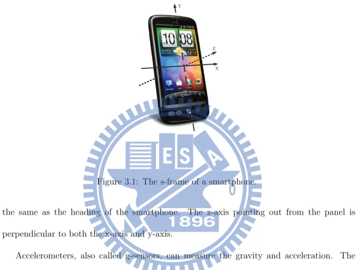
be known from the sensor specification. The relation between the x-axis, y-axis and z-axis follows Fleming’s right hand rule. For example, Fig. 3.1 illustrates the s-frame of a smartphone. The x-axis points to the right side of the panel, the direction of y-axis is
Y
Z
X
Figure 3.1: The s-frame of a smartphone.
the same as the heading of the smartphone. The z-axis pointing out from the panel is perpendicular to both the x-axis and y-axis.
Accelerometers, also called g-sensors, can measure the gravity and acceleration. The readings of g-sensors are the sum of the acceleration and the negative of the gravity. Let g denote the reading of a g-sensor, a denote the acceleration, and G denote the gravity. The relation between them can be modeled as
g = a− G.
m/s2. According to Fig. 3.2, the waveform in Block I is collected as the smartphone is placed -15 -10 -5 0 5 10 15 1 51 101 151 201 251 Ac c e ler at ion (m /s 2) Time (s) x y z I II III
Figure 3.2: A waveform of g-sensor readings.
horizontally; the waveform in Block II is collected after the smartphone is rotated clockwise 90◦; and the waveform in Block III is collected as the smartphone is placed vertically and with y-axis pointing upward.
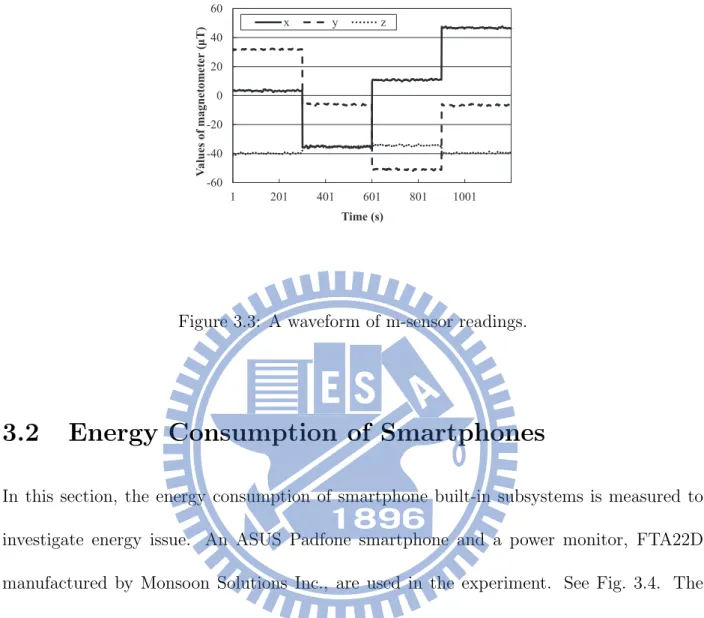
Magnetometers also called m-sensors can measure the ambient magnetic field. The ge-omagnetic field points roughly to the north pole and has intensity around 600 mGauss. The geomagnetic field is also influenced by the surrounding environments such as electrical equipments or magnetic materials. In addition, the geomagnetic field may have inclination and declination that are different from place to place. However, the magnetic declination and magnetic inclination can be ignored in low-latitude areas. Fig. 3.3 illustrates a wave-form of m-sensor readings. The x-axis is the sequence number of the readings at sampling rate 40 Hz, and y-axis is the magnitude of the magnetic field in µT.1 The orientation of a
smartphone can be calculated based on the readings of g-sensors and m-sensors. -60 -40 -20 0 20 40 60 1 201 401 601 801 1001 V al u es of m ag n et om et er ( μ T ) Time (s) x y z
Figure 3.3: A waveform of m-sensor readings.
3.2
Energy Consumption of Smartphones
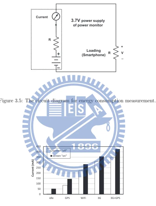
In this section, the energy consumption of smartphone built-in subsystems is measured to investigate energy issue. An ASUS Padfone smartphone and a power monitor, FTA22D manufactured by Monsoon Solutions Inc., are used in the experiment. See Fig. 3.4. The battery of the smartphone is removed, and the smartphone is driven by a 3.7 volts power supply of the power monitor. The current of the power supply is measured to record the energy consumption of the smartphone. See Fig. 3.5. Individual subsystems are alternatively turned on/off to measure the incremental current. Fig. 3.6 depicts the average current over 50000 data samples. For communication subsystems, the bars marked with triangles are the current incremental after turning on each subsystem, and the bars marked with circles are
Figure 3.4: The devices for energy consumption measurement.
representing for after turning on and executing file transfer.The sampling rate of the IMU subsystem can be set by the ”rate” parameter of the function call
android.hardware.SensorManager.registerListener( SensorEventListener listener,
Sensor sensor,
int rate)
Possible values for the ”rate” parameter includes
SensorManager.SENSOR DELAY FASTEST, SensorManager.SENSOR DELAY GAME, SensorManager.SENSOR DELAY UI, and SensorManager.SENSOR DELAY NORMAL.
The parameter basically sets an extra delay before next sampling. The corresponding extra delays are 0 µs, 20000 µs, 60000 µs and 200000 µs, respectively, and the corresponding
Loading (Smartphone) 3.7V power supply of power monitor Current R V R + _
Figure 3.5: The circuit diagram for energy consumption measurement.
0 50 100 150 200 250 300 350 400 450 idle GPS WiFi 3G 3G+GPS C u rre n t (mA ) screen "off" screen "on"
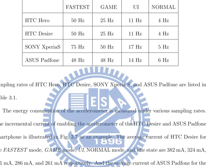
Table 3.1: The IMU sampling rates under various delay setting.
FASTEST GAME UI NORMAL
HTC Hero 50 Hz 25 Hz 11 Hz 4 Hz
HTC Desire 50 Hz 25 Hz 11 Hz 4 Hz
SONY XperiaS 75 Hz 50 Hz 17 Hz 5 Hz
ASUS Padfone 48 Hz 48 Hz 14 Hz 6 Hz
sampling rates of HTC Hero, HTC Desire, SONY Xperia S, and ASUS Padfone are listed in Table 3.1.
The energy consumption of the accelerometer is measured under various sampling rates. The incremental current of enabling the accelerometer of the HTC Desire and ASUS Padfone smartphone is illustrated in Fig. 3.7 as an example. The average current of HTC Desire for the FASTEST mode, GAME mode, UI, NORMAL mode, and idle state are 382 mA, 324 mA, 301 mA, 286 mA, and 261 mA respectively. And the average current of ASUS Padfone for the FASTEST mode, GAME mode, UI, NORMAL mode, and idle state are 209 mA, 202 mA,
121 mA, 87 mA, and 52 mA respectively. Therefore, the lower sampling rate is set, the less energy is consumed. Actually, that is to say that around 55% power consumption can be saved when reducing the sampling rate from FASTEST (48Hz) to UI (14Hz). Compared with the energy consumption of other subsystems, the energy consumption of the IMU subsystem should not be ignored.
0 50 100 150 200 250 300 350 400 450
FASTEST GAME UI NORMAL Idle
C urrent (mA ) Frequency mode HTC Desire ASUS Padfone
Figure 3.7: Incremental current of enabling the IMU of the HTC Desire and ASUS Padfone smartphone.
3.2.1
Lifetime of Battery
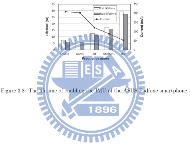
Fig. 3.8 shows the eatimated lifetime and real lifetime of ASUS Padfone smartphone under different frequency modes as well as the incremental current. The battery lifetime (in hour) is calculated in terms of battery capacity (in mAh) and average current consumption (mA)
Battery lifetime (hr) = Battery capacity (mAh)
Average current consumption (mA)
For ASUS Padfone smartphone, the battery capacity of ASUS Padfone Li-ion battery is 1520 mAh, the estimated lifetime of battery for the FASTEST mode, GAME mode, UI mode, NORMAL mode, and idle state are 7.26 hr, 7.5hr, 12.51 hr, 17.31 hr, and 29.19 hr, re-spectively, as shown in the white bar. However, the real lifetime of battery for the FASTEST mode, GAME mode, UI mode, NORMAL mode, and idle state are 5.95 hr, 5.98 hr, 11.01 hr, 15.87 hr, and 27.35 hr, respectively, as shown in the gray bar. There is a slight gap between
the real lifetime and estimated lifetime, and generally people speculated that smartphone always has self-protection mechanism for normally system shutting-down in the low-battery condition, and it is possible and reasonable that the capacity of Li-ion battery usually can not reach 100% usage. In the real situation, the real lifetime is around 1.5 hr lower than the estimated lifetime. 0 50 100 150 200 250 0 5 10 15 20 25 30 35
FASTEST GAME UI NORMAL idle
Curre nt (mA ) Lif etime (hr) Frequency mode Est. lifetime Real lifetime Current
Chapter 4
Proposed Low Sampling Rate
IMU-based Pedestrian Trajectory
System
A pedestrian trajectory can be sketched stride-by-stride based on the stride length and walking direction of each step. To implement the idea, we not only need to be aware of the occurances of stepping but also need to know the stride length and walking direction. A Pedestrian Trajectory System is designed for handheld devices to sketch pedestrian trajec-tories by detecting stepping and estimating the stride length and walking direction from the output of embedded inertial sensors. The proposed PTS consists of three modules, including the Stepping Aware Module (SAM), the Stride Length Module (SLM), and the Walking Di-rection Module (WDM), to provide the three essential information respectively. Finally, the
Dead Reckoning Module (DRM) determines the pedestrian trajectory. Fig. 4.1 illustrates the architecture of the proposed PTS.
Acceleration Magnetic intensity Step Count Stride Length Walking Direction Parameters Walking Direction Module (WDM) Stepping Aware Module (SAM) Processed acceleration Stride Length Module (SLM) Dead Reckoning Module (DRM) Trajectory
Figure 4.1: The system architecture of the proposed PTS.
SAM scans and processes the output of the accelerometer to detect the occurrence of stepping. If a stepping is detected, SLM and WDM are triggered to estimate the stride length and calculate the walking direction. SLM estimates the stride length by regression based on the parameters from SAM; and WDM calculates the walking direction based on the output of the magnetometer and processed data from SAM. The details of each module are going to be revealed in the following subsections. An example of the output of PTS is illustrated in Fig. 5.7.
4.1
Stepping Aware Module (SAM)
Let gi be the i-th reading of the g-sensor for i = 1, 2, ..., and g0 especially denote the gravity measured by the g-sensor at a static state. If the orientation of the g-sensor is not changed during the measurement especially in the vertical direction, then ai = gi −
g0 is the acceleration experienced by the smartphone. In SAM, gi is decomposed into a vertical component and a horizontal component, respectively denoted by g⊥i and g=i . The vertical component g⊥i is the projection of gi onto the direction of the gravity, and the
horizontal component g=
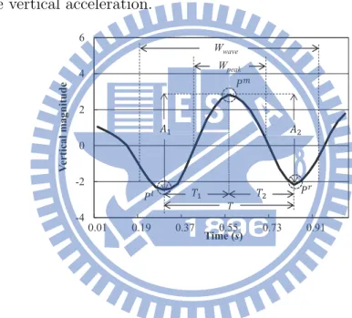
i can be obtained by g=i = gi− g⊥i . Let a⊥i denote the magnitude of the acceleration in the vertical direction. The magnitude of the vertical direction can be calculated from a⊥i = ∥g0∥ − gi · g0/∥g0∥. A typical waveform of the vertical acceleration is illustrated in Fig. 4.2 in which the x-axis represents time and the y-axis represents the magnitude of the vertical acceleration.
-4 -2 0 2 4 6 0.01 0.19 0.37 0.55 0.73 0.91 V er tic al m agn itud e Time (s) Wwave Wpeak
Figure 4.2: A waveform of the vertical acceleration
For later discussion, we introduce some waveform features of vertical acceleration. Wpeak and Wwave are two system parameters. Pm = (tm, am) in the waveform is called a local
maximum if am is the greatest value for t ∈ [tm−21Wpeak, tm+12Wpeak ]
. Pl = (tl, al)
in the waveform is called the left local minimum of Pm if al is the least value for t ∈ [
Pm if ar is the least value for t∈[tm, tm+ 1 2Wwave
]
. Wpeak is used to define local minimum, and Wwave should be large enough to contain a waveform. In most cases, a pedestrian takes at most two steps per second even in running or going upstairs and downstairs. Therefore, Wwaveis set to 0.5 second, and Wpeak is set to 0.25 second. Let N =
⌈1
2Wwave× f ⌉
− 1 where f is the sampling frequency, and i0 denote the time sequence index of Pm. For a given
Pl-Pm-Pr wave, we define some features for the recognition of stride waveform patterns,
including T1 = tm− tl, T2 = tr− tm, T = T1+ T2, A1 = am− al, A2 = am− ar, A = A1+ A2, I = 1 2N + 1( i∑0+N n=i0−N ∥g= n∥), X1 = 2N ∑ n=0 a⊥n+(i0−N)e−i2N +12π n .
T1 and T2 are respectively the left and right time span from the local maximum to the nearby
local minima, and T is the time span of the waveform. A1 and A2 are respectively the left and right amplitude of the waveform. I is the average intensity of the horizontal acceleration component. X1 is the magnitude of frequency 1 in the Discrete Fourier Transform (DFT).
The features of a stride waveform should fall in a reasonable range. A2, A, T1, T2, T , I and X1 are selected to verify whether a waveform is caused by stepping. Let Amin2 and Amax2 (and respectively Amin, Amax; T1min, T1max; T2min, T2max; Tmin, Tmax; Imin, Imax; X1min, X1max ) be the lower bound and upper bound of the range of A1 (and respectively A, T1, T2, T , I, X1). A voting-based algorithm is applied to verify whether a waveform is caused by stepping.
In our algorithm, a local maximum Pm is first identified, and then the left local minimum
Pl and right local minimum Pr of Pm are found. The Pl-Pm-Pr waveform is recognized as
a stepping waveform only if at least four out of the following seven conditions are satisfied, including A1 ∈ [ Amin1 , Amax1 ], A∈[Amin, Amax], T1 ∈ [ T1min, T1max], T2 ∈ [ T2min, T2max], T ∈[Tmin, Tmax], I ∈[Imin, Imax], X1 ∈ [ X1min, X1max].
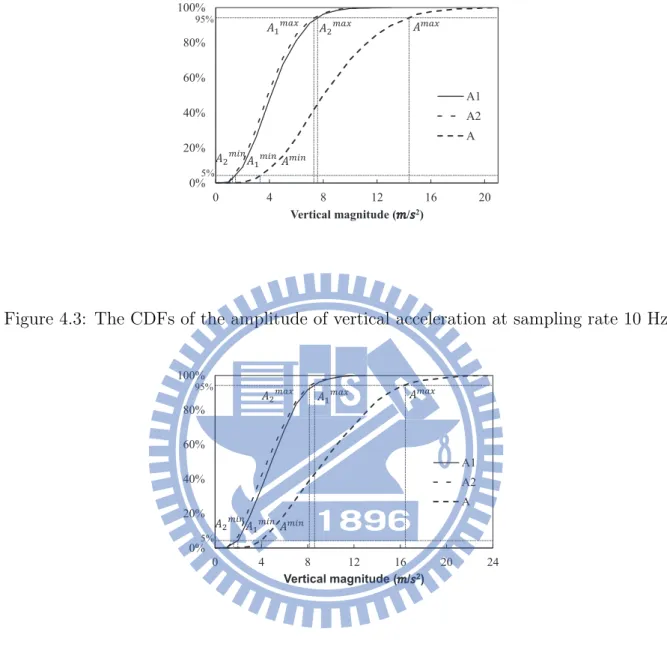
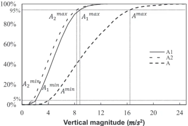
The remaining issue is how to decide those upper bounds and lower bounds. For each feature, the values corresponding to 5% and 95% in the Cumulative Distribution Function (CDF) are chosen to be the lower bound and the upper bound. To depict the CDFs, nine experiments were implemented to collect the data. In each experiment, the data of 15 steps were collected. So, totally, 135 stepping records were collected to depict the CDFs. The experiment includes walking on ground with stride length about 40 cm, 50 cm, 60 cm, 70 cm and 80 cm. For sampling rate 10 Hz, 20 Hz and 40 Hz, the CDFs of A1, A2, A are plotted in Fig. 4.3, Fig. 4.4 and Fig. 4.5; the CDFs of T1, T2, T are plotted in Fig. 4.6, Fig. 4.7 and Fig. 4.8; and the CDFs of I are respectively plotted in Fig. 4.9, Fig. 4.10 and Fig. 4.11; and
the CDFs of X1 are respectively plotted in Fig. 4.12, Fig. 4.13 and Fig. 4.14. 0% 20% 40% 60% 80% 100% 0 4 8 12 16 20 Vertical magnitude (݉/ݏ2) A1 A2 A 95% 5%
Figure 4.3: The CDFs of the amplitude of vertical acceleration at sampling rate 10 Hz.
0% 20% 40% 60% 80% 100% 0 4 8 12 16 20 24 Vertical magnitude (݉/ݏ2) A1 A2 A 95% 5%
Figure 4.4: The CDFs of the amplitude of vertical acceleration at sampling rate 20 Hz.
For example, from Fig. 4.3, we can see Amin
1 , Amax1 , Amin2 , Amax2 , Amin and Amax are 1.55, 7.76, 1.52, 7.42, 3.48 and 14.57, respectively. The thresholds (lower bounds and upper bounds) obtained from our experiments are listed in Table 4.1.
0% 20% 40% 60% 80% 100% 0 4 8 12 16 20 24 Vertical magnitude (݉/ݏ2) A1 A2 A 95% 5%
Figure 4.5: The CDFs of the amplitude of vertical acceleration at sampling rate 40 Hz.
0% 20% 40% 60% 80% 100% 0 0.2 0.4 0.6 0.8 1 Time duration (ݏ) T1 T2 T 95% 5%
Figure 4.6: The CDFs of the time duration of vertical acceleration waveforms at sampling rate 10 Hz.
0% 20% 40% 60% 80% 100% 0 0.2 0.4 0.6 0.8 Time duration (ݏ) T1 T2 T 95% 5%
Figure 4.7: The CDFs of the time duration of vertical acceleration waveforms at sampling rate 20 Hz. 0% 20% 40% 60% 80% 100% 0 0.2 0.4 0.6 0.8 Time duration (ݏ) T1 T2 T 95% 5%
Figure 4.8: The CDFs of the time duration of vertical acceleration waveforms at sampling rate 40 Hz.
0% 20% 40% 60% 80% 100% 0 0.6 1.2 1.8 2.4 3 3.6 4.2 I (݉/ݏ2) 95% 5 %
Figure 4.9: The CDF of the average intensity of the horizontal acceleration component at sampling rate 10 Hz. 0% 20% 40% 60% 80% 100% 0 0.6 1.2 1.8 2.4 3 3.6 I (݉/ݏ2) 95% 5 %
Figure 4.10: The CDF of the average intensity of the horizontal acceleration component at sampling rate 20 Hz.
0% 20% 40% 60% 80% 100% 0 0.6 1.2 1.8 2.4 3 3.6 I (݉/ݏ2) 95% 5 %
Figure 4.11: The CDF of the average intensity of the horizontal acceleration component at sampling rate 40 Hz. 0% 20% 40% 60% 80% 100% 0 6 12 18 X1(݉/ݏ2) 95% 5%
0% 20% 40% 60% 80% 100% 0 6 12 18 24 30 36 X1(݉/ݏ2) 95% 5%
Figure 4.13: The CDF of the magnitude of DFT on frequency of 1 at sampling rate 20 Hz.
0% 20% 40% 60% 80% 100% 0 18 36 54 72 X1(݉/ݏ2) 95% 5%
Table 4.1: The thresholds used in SAM.
10(Hz) 20(Hz) 40(Hz)
min max min max min max
A1 (m/s2) 1.55 7.76 2.06 8.61 2.15 8.98 A2 (m/s2) 1.52 7.42 1.82 8.37 1.72 8.37 A (m/s2) 3.48 14.57 4.19 16.53 4.24 16.77 T1 (s) 0.1 0.41 0.1 0.37 0.08 0.35 T2 (s) 0.1 0.51 0.16 0.43 0.1 0.4 T (s) 0.4 0.71 0.38 0.65 0.36 0.62 I (m/s2) 0.58 2.23 0.60 1.8 0.6 1.8 X1 (m/s2) 1.30 10.34 2.24 20.12 3.79 38
Table 4.2: The covariance between the stride length and waveform features. 10(Hz) 20(Hz) 40(Hz) A1 0.5 0.55 0.53 A2 0.46 0.53 0.5 A 0.52 0.56 0.55 T1 0.19 0.24 0.25 T2 0.08 0.07 0.06 T 0.26 0.32 0.32 I 0.38 0.38 0.37 X1 0.55 0.61 0.61
4.2
Stepping Length Module (SLM)
The features calculated by SAM will be used for SLM to estimate the stride length by regression methods. The two most related features to the stride length are figured out first. Let D denote the stride length. The covariance between the stride length D and the features A1, A2, A, T1, T2, T , I and X1 are calculated from the data collected in the previous subsection. Note that since the stride length is not meaningful in the upstairs and downstairs experiments, the data collected in the two cases are not considered in the analysis. According to the covariance listed in Table 4.2, A and X1 are the two most correlated parameters to the stride length. Therefore, A and X1 are chosen to be used in the regression analysis.
We apply double variable linear regression and double variable quadratic regression on A and X1 to estimate the stride length D. Let DL and DQ denote the estimated stride length obtained by the linear regression and quadratic regression. The linear regression equation is
DL = pL1 + pL2A + pL3X1,
and the quadratic regression equation is
DQ= pQ1 + pQ2A + pQ3X1+ p Q 4AX1+ p Q 5A 2 + pQ6X12.
Table 4.3 gives the coefficients obtained in the regression analysis based on our experiment data. The RMSEs under sampling rate 10 Hz in the regression analysis are 13.03 and 12.99 for the linear equation and quadratic equation respectively; the RMSEs under sampling rate 20 Hz in the regression analysis are 12.33 and 12.21 for the linear equation and quadratic equation, and the RMSEs under sampling rate 40 Hz in the regression analysis are 12.32 and 12.15 for the linear equation and quadratic equation, respectively. Fig. 4.15, Fig. 4.16, and Fig. 4.17 illustrate all the experiment data and the regression equations in which the x-axis, y-axis and z-axis represent the magnitude of DFT on frequency of 1 for sampling rate 10 Hz, 20 Hz and 40 Hz, the amplitude of vertical acceleration and the experiment of different stride length, respectively. The circles represent the experiment data, the dashed line depicts the linear regression equation, and the solid curve depicts the quadratic regression equation.
Table 4.3: Coefficients obtained in the regression analysis. Linear regression pL 1 pL2 pL3 10(Hz) 52.15 0.08 1.81 20(Hz) 50.01 -0.10 1.23 40(Hz) 50.66 -0.42 0.75 Quadratic regression pQ1 pQ2 pQ3 pQ4 pQ5 pQ6 10(Hz) 54.56 -1.12 2.64 0.03 0.06 -0.11 20(Hz) 51.95 -1.89 2.42 -0.07 0.14 -0.02 40(Hz) 54.49 -2.90 1.50 -0.02 0.15 -0.01
80 70 50 60 40 0 3 6 9 12 15 18 21 0 4 8 12 16 Stri d e l eng th (c m )
Stride length vs. A & X1 Linear regression Quadratic regression
10 Hz
Figure 4.15: The regression analysis of SLM at 10 Hz.
80 70 50 60 40 0 3 6 9 12 15 18 21 0 4 8 12 16 Stri d e l eng th (c m )
Stride length vs. A & X1 Linear regression Quadratic regression
20 Hz
80 70 50 60 40 0 3 6 9 12 15 18 21 0 4 8 12 16 Stri d e l eng th (c m )
Stride length vs. A & X1 Linear regression Quadratic regression
40 Hz
Figure 4.17: The regression analysis of SLM at 40 Hz.
4.3
Walking Direction Module (WDM)
The coordinate system used in the readings of sensors is called the sensor frame or s-frame in short and is defined by hardware manufacturers. The definition of the s-frame can be found from hardware specification and usually follows the right hand rule. The tangent frame or local level horizontal frame is called the Earth frame or e-frame in short and is used in tracking objects moving on the ground and depicting pedestrian trajectories on maps. The x-axis, y-axis and z-axis of the e-frame respectively point to the north, east and center of the Earth. If the walking direction of a pedestrian is aligned with the heading of the handheld device, the walking direction is the yaw angle from the e-frame to the s-frame. The angle is also called the heading angle.
denotes the coordinate transformation matrix that transforms the reading of the sensor from the s-frame to the e-frame. In other words, if v is a vector, we have
[v]E = TS→E[v]S
where [v]S is the coordinate of v observed from the s-frame and [v]E is the coordinate of v observed from the e-frame. Assume the gravity points exactly to the center of the Earth and the magnetic field points exactly to the north and maybe with some inclination. Then, we have I = TS→E [ g×(m×g) ∥g×(m×g)∥ ∥m×g∥m×g −∥g∥g ] , and therefore TS→E = [ g×(m×g) ∥g×(m×g)∥ ∥m×g∥m×g −∥g∥g ]−1 = [ g×(m×g) ∥g×(m×g)∥ ∥m×g∥m×g −∥g∥g ]T .
Let ψ, θ and ϕ respectively denote the yaw angle, pitch angle and roll angle of Euler angles. Based on the Yaw-Pitch-Roll conversion, we have
TS→E = cψcθ −sψcϕ + cψsθsϕ sψsϕ + cψsθcϕ sψcθ cψcϕ + sψsθsϕ −cψsϕ + sψsθcϕ −sθ cθsϕ cθcϕ
where c is shorthand for cos and s is shorthand for sin. Therefore, the yaw angle can be obtained from
ψ = arctan[TS→E]2,1 [TS→E]1,1
Chapter 5
Experiment Results
5.1
Performance Evaluation of Individual Modules
SAM was evaluated first. Eight people were invited to join in the experiment. Testers held the device and then took 100 steps casually. Each tester did the experiment three times. One is for the IMU running at 10 Hz, another is for the IMU running at 20 Hz and the other is for the IMU running at 40 Hz. The number of detected steps for each person are listed in Fig. 5.1. Based on the result, the inaccuracy rates under sampling rate 10 Hz, 20 Hz and 40 Hz are 2.63%, 4.13% and 4.13% respectively.
Then, we evaluated the performance of SLM. In the experiment, people were asked to walk with a fixed stride length, including 40 cm, 50 cm, 60 cm, 70 cm and 80 cm. SLM estimated the stride length of each step. Data were grouped by the real stride length. The result is illustrated in Fig. 5.2 in which x-axis denotes the real stride length and y-axis
50 75 100 125 150 A B C D E F G H Numb e r of e s tima ted s teps Testers 10 Hz 20 Hz 40 Hz
Figure 5.1: The number of detected steps out of 100 steps.
denotes the estimated stride length. In each group, the black box denotes the interquartile
30 40 50 60 70 80 90 40 50 60 70 80 E stim a te d stri d e le n g th (cm ) Stride length (cm) 10 Hz 20 Hz 40 Hz
Figure 5.2: The error box of estimated stride length.
range (IQR) of estimated stride length at sampling rate 10 Hz, the gray box denotes the (IQR) of estimated stride length at sampling rate 20 Hz, the white box denotes the IQR of the estimated stride length at sampling rate 40 Hz, and the lines mark the range of the estimated stride length. Based on the result, the average errors of SLM under sampling rate 10 Hz, 20 Hz and 40 Hz are 20.66%, 18.72% and 18.43% respectively. In addition, eight
people used our PTS to walk along one 20 m straight line. The total distance estimated by SLM for each person is shown in Fig. 5.3.
12 14 16 18 20 22 24 26 28 A B C D E F G H E s tima ted dis tanc e (m) Testers 10 Hz 20 Hz 40 Hz
Figure 5.3: Total estimated distance by SLM under 20 m walk.
According to the result, the overall accuracy rate of SLM under sampling rate 10 Hz, 20 Hz and 40 Hz are 4.4%, 4.59% and 3.59% respectively.
The performance of WDM is also verified. Fig. 5.4, Fig. 5.5 and Fig. 5.6 illustrate the walking direction of each step in a PTS experiment with different sampling rate.
0 90 180 270 360 1 51 101 151 201 251 A zimut h (deg) Steps Expriment Direction Real Direction
0 90 180 270 360 1 51 101 151 201 251 A zimuth (d e g) Steps Expriment Direction Real Direction
Figure 5.5: The walking direction of each step at 20 Hz.
0 90 180 270 360 1 51 101 151 201 251 A zimuth (d e g) Steps Expriment Direction Real Direction
In Fig. 5.4, Fig. 5.5 and Fig. 5.6, the x-axis is the sequence number of each step and y-axis is the azimuth of each step. The solid line denotes the real walking direction, and the dashed line denotes the estimated walking direction. Based on the result, the errors of WDM under sampling rate 10 Hz, 20 Hz and 40 Hz are 11.43 degrees, 11.96 degrees and 13.87 degrees in average, respectively.
5.2
Implementation of the Proposed PTS
A PTS with graphic user interfaces was implemented on Android smartphones. To evaluate the performance of the prototype system, testers held the smartphone and walked in the building. 24 reference points were marked on the floor, and the average distance between two neighboring reference points is around 5 m. The positioning errors at these reference points were recorded. Fig. 5.7, Fig. 5.8 and Fig. 5.9 illustrate the experiment environment.
10 Hz Real Path PTS Path
Figure 5.7: A experiment result of the proposed PTS at 10 Hz.
20 Hz Real Path PTS Path
Figure 5.8: A experiment result of the proposed PTS at 20 Hz.
40 Hz Real Path PTS Path
the reference points. In addition, the green line is an example of the trajectory calculated by the system, and the green dots denote the estimated position of these reference points. Fig. 5.10 is the CDFs of the positioning errors at these reference points.
0% 20% 40% 60% 80% 100% 0 1 2 3 4 5 6 7 8 9 10 11 12 13 Distance error (m) 10 Hz 20 Hz 40 Hz
Figure 5.10: The CDFs of positioning errors of the proposed PTS.
According to our experiment results, 80% of the positioning errors are within 4.8 m, 5.8 m and 5.2 m.
Chapter 6
Conclusions
Energy consumption is an important issue for battery-powered handheld devices. Applica-tions developed for smartphones should keep energy consumption as a major consideration. The energy consumption of various embedded subsystems of smartphones was measured, and the results show that the energy consumption of the IMU subsystem should not be ig-nored. Based on this observation, in this work, we developed a low sampling rate IMU-based pedestrian trajectory system for smartphones. The proposed PTS was implemented with a graphic user interface on an Android platform. Based on our experiment results, if the starting position of a pedestrian trajectory is given, applying dead reckoning, 80% of the positioning errors are within 4.8 m, 5.8 m and 5.2 m under sampling rate 10 Hz, 20 Hz and 40 Hz respectively. In addition, the results show that reducing the sampling rate of the IMU from FASTEST (48Hz) to UI (14Hz) can not only get about 55% lower power consumption but still achieve similar positioning accuracy.
Bibliography
[1] E. Foxlin, “Pedestrian tracking with shoe-mounted inertial sensors,” IEEE Computer Graphics and Applications, vol. 25, no. 6, pp. 38–46, November 2005.
[2] L. Ojeda and J. Borenstein, “Personal dead-reckoning system for GPS-denied environ-ments,” in Proceedings of the 2007 IEEE International Workshop on Safety, Security and Rescue Robotics (SSRR 2007), 27-29 September 2007, pp. 1–6.
[3] C.-M. Su, J.-W. Chou, C.-W. Yi, Y.-C. Tseng, and C.-H. Tsai, “Sensor-aided personal navigation systems for handheld devices,” in Proceedings of the 39th International Con-ference on Parallel Processing Workshops (ICPPW 2010), 13-16 September 2010, pp.
533–541.
[4] A. Anand, C. Manikopoulos, Q. Jones, and C. Borcea, “A quantitative analysis of power consumption for location-aware applications on smart phones,” in Proceedings of the 2007 IEEE International Symposium on Industrial Electronics (ISIE 2007), 4-7
[5] M. B. Kjasrgaard, “Location-based services on mobile phones: minimizing power con-sumption,” IEEE Pervasive Computing, vol. 11, no. 1, pp. 67–73, 2012.
[6] N. F. Krasner, S. Carlos, and Calif, “GPS receiver utilizing a communcation link,” U.S. Patent US005 841 396A, 1998.
[7] D. Pozar and S. Duffy, “A dual-band circularly polarized aperture-coupled stacked mi-crostrip antenna for global positioning satellite,” IEEE Transactions on Antennas and Propagation, vol. 45, no. 11, pp. 1618–1625, November 1997.
[8] P. Bahl and V. N. Padmanabhan, “RADAR: an in-building RF-based user location and tracking system,” in Proceedings of the 19th Annual Joint Conference of the IEEE Computer and Communications Societies (IEEE INFOCOM 2000), vol. 2, 26-30 March
2000, pp. 775–784.
[9] M. Youssef and A. Agrawala, “The Horus WLAN location determination system,” in Proceedings of the 3rd International Conference on Mobile Systems, Applications and
Services (ACM MobiSys 2005), 6-8 June 2005, pp. 205–218.
[10] K. Chintalapudi, A. P. Iyer, and V. N. Padmanabhan, “Indoor Localization Without the Pain,” in Proceedings of the 16th Annual International Conference on Mobile Computing and Networking (ACM MobiCom 2010), 20-24 September 2010, pp. 173–184.
[11] S. Sen, R. R. Choudhury, B. Radunovi´c, and T. Minka, “You are Facing the Mona Lisa: Spot Localization using PHY Layer Information,” in Proceedings of the 10th
Interna-tional Conference on Mobile Systems, Applications and Services (ACM MobiSys 2012),
25-29 June 2012, pp. 183–196.
[12] J. Kim and H. Jun, “Vision-based location positioning using augmented reality for indoor navigation,” IEEE Transactions on Consumer Electronics, vol. 54, no. 3, pp. 954–962, August 2008.
[13] L. C. Huey, P. Sebastian, and M. Drieberg, “Augmented reality based indoor positioning navigation tool,” in Proceedings of the 2011 IEEE Conference on Open Systems (ICOS 2011), 25-28 September 2011, pp. 256–260.
[14] Y.-C. Cheng, J.-Y. Lin, C.-W. Yi, Y.-C. Tseng, L.-C. Kuo, Y.-J. Yeh, and C.-W. Lin, “AR-based positioning for mobile devices,” in Proceeding of the 40th International Conference on Parallel Processing Workshops (ICPPW 2011), 13-16 September 2011,
pp. 63–70.
[15] J.-Y. Lin, Y.-C. Tseng, and C.-W. Yi, “PEAR: personal evacuation and rescue sys-tem,” in Proceedings of the 6th ACM workshop on Wireless multimedia networking and computing (WMuNeP 2011), 31 October - 4 November 2011.
[16] C.-C. Lo, C.-P. Chiu, Y.-C. Tseng, S.-A. Chang, and L.-C. Kuo, “A walking velocity update technique for pedestrian dead-reckoning applications,” in Proceeding of the 22nd Annual IEEE International Symposium on Personal Indoor and Mobile Radio
[17] I. Constandache, R. Choudhury, and I. Rhee, “Towards mobile phone localization with-out war-driving,” in Proceedings of the 29th Conference on Computer Communications (IEEE INFOCOM 2010), 14-19 March 2010, pp. 1–9.
[18] C.-W. Yi, C.-M. Su, W.-T. Chai, J.-L. Huang, and T.-C. Chiang, “constellations: G-sensor motion tracking systems,” in Proceeding of the IEEE 71st Vehicular Technology Conference (VTC 2010-Spring), 16-19 May 2010, pp. 1–5.
[19] H. Wang, S. Sen, A. Elgohary, M. Farid, M. Youssef, and R. R. Choudhury, “No need to war-drive: Unsupervised Indoor Localization,” in Proceedings of the 10th International Conference on Mobile Systems, Applications and Services (ACM MobiSys 2012), 25-29
June 2012, pp. 197–210.
[20] P.-L. Shih, P.-J. Chiu, Y.-C. Cheng, J.-Y. Lin, and C.-W. Yi, “Energy-Aware Pedestrian Trajectory System,” in Proceeding of the 41th International Conference on Parallel Processing Workshops (ICPPW 2012), 10-13 September 2012, pp. 514–523.