可容忍高時脈誤差之全數位時序同步研究

國 立 交 通 大 學

資訊科學與工程研究所

碩 士 論 文

可容忍高時脈誤差之全數位時序同步研究

The Study of Digital Timing Recovery

For

Wide Clock Offset Tolerance

研 究 生：王偉任

指導教授：許騰尹博士

可容忍高時脈誤差之全數位時序同步研究

The Study of Digital Timing Recovery

For

Wide Clock Offset Tolerance

研 究 生：王偉任 Student：Wei-Ren Wang

指導教授：許騰尹 博士

Advisor : Terng-Yin Hsu

國 立 交 通 大 學

資 訊 科 學 與 工 程 研 究 所

碩 士 論 文

A Thesis

Submitted to Institute of Computer Science and Engineering College of Computer Science

National Chiao Tung University in partial Fulfillment of the Requirements

for the Degree of Master

in

Computer Science June 2008

Hsinchu, Taiwan, Republic of China

Contents

page

Abstract...iv

Chapter 1 Introduction...1

Chapter 2 System Platform...3

2.1 IEEE 802.11n PHY Specification ...3

2.1.1 Transmitter ...3

2.1.2 Receiver ...4

2.1.3 Basic MIMO PPDU Format...4

2.2 Channel model ...5

2.2.1 Additive White Gaussian Noise...5

2.2.2 Multipath...7

2.2.3 Carrier Frequency Offset ...9

2.2.4 Sampling Clock Offset...11

Chapter 3 Proposed Algorithm ...14

3.1 Coarse timing synchronization of Wide Clock Offset ...15

3.2 Fine timing synchronization of Wide Clock Offset ...20

Chapter 4 Simulation result ...23

4.1 Simulation Environment ...23

4.2 Simulation Result...25

4.3 Simulation analysis ...29

Chapter 5 The Proposed Architecture ...30

Chapter 6 Conclusion and Future Work ...32

6.1 Conclusion ...32

6.2 Future work...34

List of Figures

page

Figure 2-1 The MIMO-OFDM transmitter data path ...3

Figure 2-3 The Basic MIMO-OFDM PPDU format...5

Figure 2-4 The MIMO-OFDM system model ...5

Figure 2-5 The received signal with and without AWGN ...7

Figure 2-6 The signal constellation after FFT output. ...7

Figure 2-7 Multipath: origin and phenomena ...8

Figure 2-8 Instantaneous impulse responses...8

Figure 2-9 The cause of CFO and I/QMismatch ...9

Figure 2-10 The symbol rotation angle is increasing with time ...10

Figure 2-11 CFO effect under CFO 100 ppm use 64 QAM modulation ..10

Figure 2-12 An example of oversampled signal with SCO ...11

Figure 2-13 Clock drift makes constellation dispersed...12

Figure 2-14 The phase rotation on each subcarrier under SCO environment ...13

Figure 3-1 Flowchart of the proposed algorithm ...14

Figure 3-2 The three basic unit of Coarse SCO estimation ...15

Figure 3-3 R+5000 and R-5000 in each SCO quantity of 10000 packets...16

Figure 3-4 The three basic unit of fine SCO estimation ...20

Figure 3-5 R+8000 and R-8000 in each SCO quantity of 10000 packets 20 Figure 4-1 PER VS SNR of ideal and non-ideal situation...25

Figure 4-3 RMSE VS SNR of the proposed algorithm...26

Figure 4-4 PER of Each SCO ppm in different SNR...26

Fiigure 4-5 Error Probability Distribution ...27

Figure 4-6 Constellation of SCO 1000 ppm under 2x2 MIMO-OFDM system (a) w/o SCO compensation (b)with SCO compensation ...28

Figure 4-7 Constellation of SCO 5000 ppm under 2x2 MIMO-OFDM system (a) w/o SCO compensation (b)with SCO compensation ...28

Figure 4-8 Constellation of SCO 10000 ppm under 2x2 MIMO-OFDM system (a) ...28

w/o SCO compensation (b)with SCO compensation...28

Figure 5-1 Block diagram of the proposed algorithm...30

Figure 5-2 Block of SCO estimation ...30

List of Tables

page Table 3-1 The value of R+5000, R-5000 and R+－5000diff in each different SCO

quantity ...17

Table 3-2 Decision criteria of Coarse SCO estimation...18

Table 3-3 Coarse SCO estimation of 10000 packets ...18

Table 3-4 The value of R+8000, R-8000 and R+－8000diff in each different SCO quantity ...21

Table 3-5 Decision criteria of Fine SCO estimation...21

Table 3-6 Fine SCO estimation of 10000 packets ...22

Table 4-1 TGn Multipath Specifications...24

Table 4-2 MCS set ...24

The Study of Digital Timing Recovery

For

Wide Clock Offset Tolerance

Student: You-Hsien Lin

Advisor: Dr. Terng-Yin Hsu

Department of Computer Science and Information Engineering,

National Chiao Tung University

Abstract

Orthogonal frequency division multiplexing (OFDM) has been widely adopted in broadband wireless communication systems , such as 802.11a , due to it’s robustness against the effects of multipath propagation. However , OFDM systems are more sensitive to synchronization errors than single carrier systems. Timing synchronization is a crucial part of OFDM receiver design , therefore it’s one of the important tasks performed at the receiver. More specifically ., Sampling Clock Offset (SCO) , if not compensated , could lead to an unacceptable BER increase .

The proposed method before to solve sampling clock offset before can tolerate SCO + - 400ppm at most. In this thesis we proposed a method to achieve wider Clock Offset tolerance to 10000 ppm. Our platform is 2-by-2 MIMO-OFDM system set up with matlab. With this platform , our proposed algorithm could be verified and some simulation results will be shown in this thesis. By the accomplishment of these simulations, our algorithm is also verified.

Chapter 1

Introduction

ue to its high spectral efficiency and robustness to multipath fading channels , OFDM is becoming the technique of choice for high data rate transmission . OFDM is already used in digital audio broadcasting (DAB) [1] ,digital video broadcasting (DVB) [2] , Wireless Local Area Networks (WLAN) [3] , and other high speed data applications for both wireless and wired communications. OFDM is also a serious candidate to be in the standard for 4th generation (4G) mobile communication systems.

Despite its promises, OFDM is very sensitive to synchronization errors and, in the presence of such inaccuracies , the performance of an OFDM system can be greatly degraded. Two mismatches are particularly harmful to the OFDM system ; the carrier frequency offset [4] and the sampling clock offset [5]. These two offsets induce the same effects; amplitude reduction and phase rotation of the demodulated data, in addition, they destroy the orthogonality between the subcarriers, or, in other words, they generate Inter Carrier Interference (ICI). The ICI will behave like an additional noise and will therefore degrade the SNR and, a fortiori, the performance of the OFDM system. Consequently, these errors should be estimated and compensated before demodulating the data with the Discrete Fourier Transform (DFT).

Multiple-input multiple-output (MIMO) makes use of multiple transmitter and multiple receiver antennas to transmit independent data streams simultaneously for increasing diversity and spectral efficiency. Consequently, the combination of MIMO and OFDM is widely discussed in recent years and has been used by more wireless broadband systems such as IEEE 802.11n [6] and IEEE 802.16a.

A huge amount of methods have been proposed to combat the carrier frequency

offset (CFO). Both data-aided methods [7]-[9] and blind schemes [10]-[12] have been developed. However research devoted to the estimation of the sampling clock offset is rather scarce, this is surprising since, as discussed above, the SCO can be as deleterious to the OFDM system as the CFO. The proposed method before to solve sampling clock offset can tolerate SCO + - 400ppm at most. In this thesis we proposed a method to achieve wider Clock Offset tolerance to 10000 ppm.

This thesis is organized as follows. In Chapter 2, a brief introduction of MIMO-OFDM system is given, including IEEE 802.11n physical layer transmitter, receiver and wireless channel model. In Chapter 3, the proposed synchronization algorithm for 2*2 MIMO-OFDM systems is presented. The simulation results and analysis are shown in Chapter 4. Proposed hardware architectures are presented in Chapter 5. Finally, this thesis is concluded in Chapter 6 and reference is in the last part of this thesis.

Chapter 2

System Platform

N this chapter, we will introduce the basic of OFDM. MIMO-OFDM specification of IEEE 802.11n PHY layer of the TGn Sync Proposal [13] is aimed. Three main blocks of wireless communication: transmitter, receiver, PPDU format and channel model are described as follows , such as additive white Gaussian noise (AWGN) , multipath , sampling clock offset (SCO) , carrier frequency offset (CFO) , and so on.

2.1 IEEE 802.11n PHY Specification

2.1.1 Transmitter

Figure 2-1 is the transmitter block diagram. The platform we used is MIMO- OFDM , and it supports BPSK、QPSK、16-QAM、64-QAM four kinds of modulation and FEC supports 1/2、2/3、3/4、5/6 four kinds of coding rate , and it can use 2x2 or 4x4 antennas to transmit data. First of all , the bit stream is parsed into several spatial streams , according to the transmitter antenna’s number. For each spatial stream,

blocks of bits that map to a single OFDM symbol are interleaved. This interleaving

I

FE C e n c o d e r pu nc tu re s p at ia l s tre a m p ar s e

step is called ”frequency interleaving” because it results in bit interleaving across subcarriers. The combination of the spatial stream parser and the frequency interleavers results in space-time interleaving. Interleaved bits are then mapped to QAM constellation points. After QAM mapping, the constellation points pass through Space Time Block Code (STBC) encoder of Alamouti scheme. And the STBC encoder spreads the constellation points of each spatial streams to space-time streams. After STBC , data goes through OFDM modulation and transfer data from frequency domain to time domain with IFFT. In 20 MHZ , each OFDM symbol has 64 subcarriers , 52 of them are data subcarriers , 4 of them are pilots and rest of them are null subcarriers. At last the Guard Interval (GI) are inserted and the signal is transmitted by RF.

2.1.2 Receiver

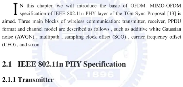
Figure 2-2 shows the receiver block diagram. In the receiver the signal received from the RF. Sync is the block where we deal with the synchronization problem including timing and frequency here. And then we use FFT to transfer the synchronized signal from time domain to frequency domain. Channel effect will be estimated and compensated by Equalizer. After all the estimation and compensation of the effect we faced , we use Alamouti STBC decoder to combine two space-time streams to single spatial streams. Then the spatial streams are demodulated to bit-level streams. And these bit streams are de-interleaved and merge to single data stream. At last, the data stream will be decoded by FEC which includes de-puncturing, Viterbi decoder and de-scrambler.

s pa tia l me rge de -p un ct u re Viterbi dec o de de-sc ram b le

Figure 2-2 The MIMO-OFDM receiver data path

2.1.3 Basic MIMO PPDU Format

The generic PPDU format is shown in Figure 2-3. The L-STF (Legacy Short Training Field), the L-LTF (Legacy Long Training Field), L-SIG (Legacy Signal Field) and HT-SIG (High Throughput Signal Field) comprise the legacy compatible part of the PPDU preamble. HT-STF, the HT-STFs and HT-Data symbols comprise the HT-Part of the PPDU. Each packet contains these header for packet detection ,

channel estimation and synchronization problems. The L-STF is formed by the repetition of ten Legacy Short Training Sequences (L-STS) of 16 samples each. And we use it to accomplish the coarse and fine estimation of Wide Clock offset issue.

Figure 2-3 The Basic MIMO-OFDM PPDU format

2.2 Channel model

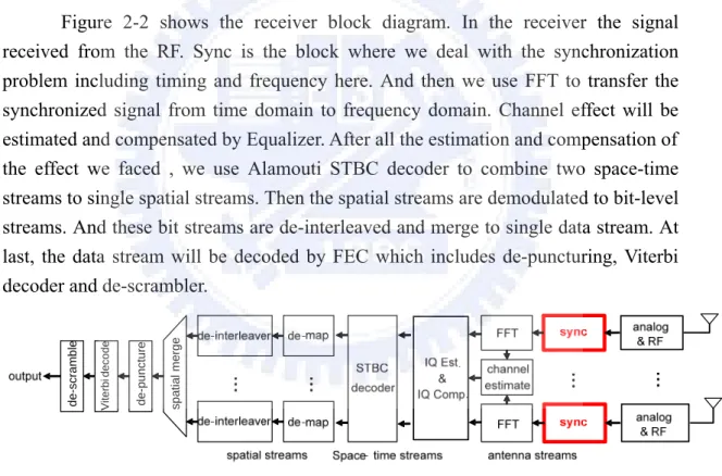
There are many imperfect effects occur while transmitted signal pass through channel such as Addictive White Gaussian Noise(AWGN), Multipath ,Carrier frequency offset (CFO) , Sampling Clock offset (SCO) , and so on. Figure 2-4 shows the system channel model. The colored blocks are the effects which we’ll introduce as follows. In the thesis , we’ll focus on the effect of red block as well as SCO.

Figure 2-4 The MIMO-OFDM system model

2.2.1 Additive White Gaussian Noise

In communications, the additive white Gaussian noise (AWGN) channel model is one in which the only impairment is the linear addition of wideband or white noise with a constant spectral density (expressed as watts per hertz of bandwidth) and a Gaussian distribution of amplitude. The model does not account for the phenomena of fading, frequency selectivity, interference, nonlinearity or dispersion. However, it produces simple, tractable mathematical models which are useful for gaining insight

into the underlying behavior of a system before these other phenomena are considered.

Wideband Gaussian noise comes from many natural sources, such as the thermal vibrations of atoms in antennas (referred to as thermal noise or Johnson-Nyquist noise), shot noise, black body radiation from the earth and other warm objects, and from celestial sources such as the sun.

The AWGN channel is a good model for many satellite and deep space communication links. It is not a good model for most terrestrial links because of multipath, terrain blocking, interference, etc. However for terrestrial path modeling, AWGN is commonly used to simulate background noise of the channel under study, in addition to multipath, terrain blocking, interference, ground clutter and self interference that modern radio systems encounter in terrestrial operation.

The signal distorted by AWGN can be derived as

( ) ( ) ( )

r t =s t +n t (2.1)

In equation (2.1), r t( ) is received signal,s t( ) is transmitted signal and n t( ) is

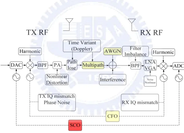
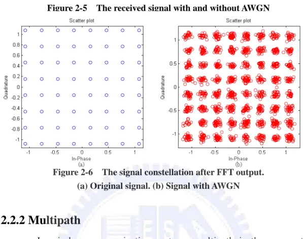
AWGN. It causes the received signal fluctuated. This effect is illustrated in Figure 2-5 and Figure 2-6. Other channel effects become more severely when AWGN joins without any compensation. A common solution but not the panacea, moving average, can just mitigate this symptom.

Figure 2-5 The received signal with and without AWGN

Figure 2-6 The signal constellation after FFT output. (a) Original signal. (b) Signal with AWGN

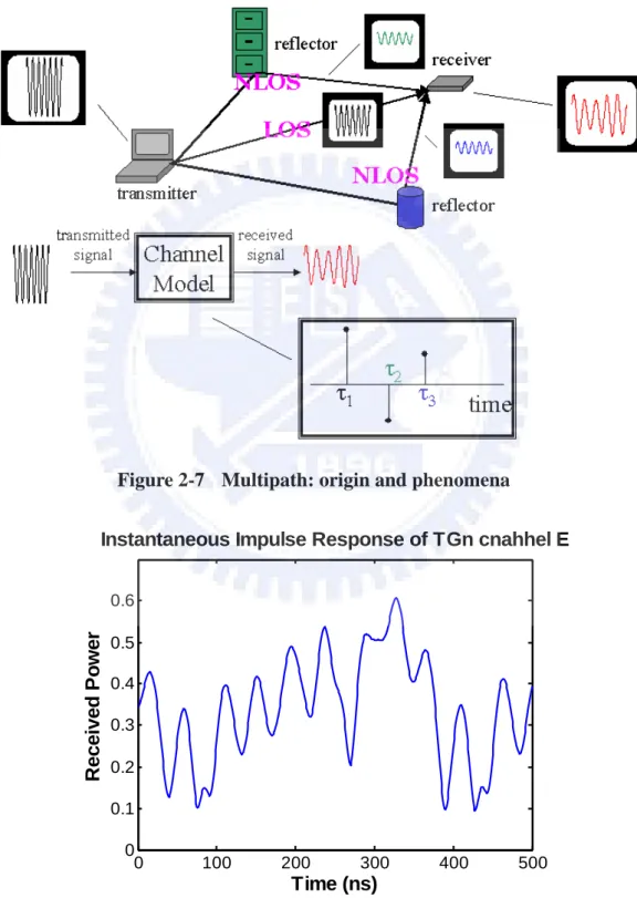
2.2.2 Multipath

In wireless communication systems, multipath is the propagation phenomenon that results in radio signals' reaching the receiving antenna by two or more paths. Causes of multipath include atmospheric ducting, ionospheric reflection and refraction, and reflection from terrestrial objects, such as mountains and buildings. And it usually goes alone with severe fading results in a signal reduction of more than 30dB. All of these signal paths are combined at the receiver to produce a signal that is a distorted version of the transmitted signal. Multi-path is usually described by two sorts:

A. Line-of-sight (LOS): the direct connection between the transmitter (TX) and the receiver (RX).

B. Non-line-of-sight (NLOS): the path arriving after reflection from reflectors. Figure 2-7 shows the origin of multipath and the corresponding effect in communications. The effects of multipath include constructive and destructive interference, and phase shifting of the signal. This causes Rayleigh fading, named after Lord Rayleigh. The standard statistical model of this gives a distribution known as the Rayleigh distribution. Rayleigh fading with a strong line of sight content is said to have a Rician distribution, or to be Rician fading. In high speed WLAN for indoor environment, multipath can cause errors and affect the quality of communications. The errors are due to inter-symbol interference (ISI) and frequency-selective fading when the maximum delay spread of the channel is larger than symbol period or

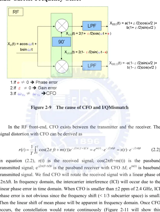
channel coherent bandwidth is smaller than data bandwidth. In IEEE 802.11n application, the receiver design must guarantee the performance under the multipath fading channel with maximum delay spread smaller than guard interval (GI) of OFDM symbol. A representation of Rayleigh fading and a measured received power-delay profile are shown in Figure 2-8.

Figure 2-7 Multipath: origin and phenomena

0 100 200 300 400 500 0 0.1 0.2 0.3 0.4 0.5 0.6 Time (ns) R e cei ved P o wer

2.2.3 Carrier Frequency Offset

Figure 2-9 The cause of CFO and I/QMismatch

In the RF front-end, CFO exists between the transmitter and the receiver. The signal distortion with CFO can be derived as

2 ( ) ( ) 2 2 0 1 ( ) Tcos(2 ( )) j f f t m t j ft ( ) j ft r t ft m t e e e s t e T π π π π − +Δ − Δ − Δ =

_∫

+ = ⋅ = ⋅ (2.2)

In equation (2.2), r(t) is the received signal; cos(2πft+m(t)) is the passband

transmitted signal; e-j2π(f+Δf)t is the passband receiver with CFO Δf; em(t) is baseband

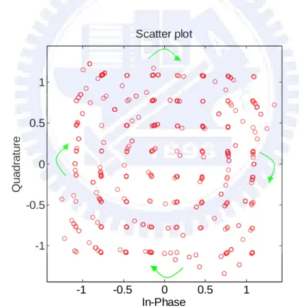
transmitted signal. We find CFO will rotate the received signal with a linear phase of -2πΔft. In frequency domain, the intercarrier interference (ICI) will occur due to the linear phase error in time domain. When CFO is smaller than ±2 ppm of 2.4 GHz, ICI phase error is not obvious since the frequency shift (< 1/3 subcarrier space) is small. Then the linear shift of mean phase will be apparent in frequency domain. Once CFO occurs, the constellation would rotate continuously (Figure 2-11 will show this phenomenon), and cause the packet error rate (PER) keeps high even when SNR increases.

Figure 2-10 The symbol rotation angle is increasing with time

AFC is the most common circuit that maintains the frequency of an oscillator within the specified limits with respect to a reference frequency. With this powerful device, we can easily compensate our performance loss due to CFO.

Figure 2-11 CFO effect under CFO 100 ppm use 64 QAM modulation

-1 -0.5 0 0.5 1 -1 -0.5 0 0.5 1 Quadrat u re In-Phase Scatter plot

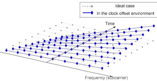
2.2.4 Sampling Clock Offset

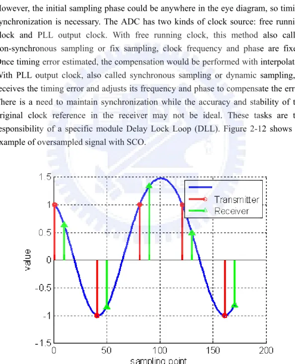
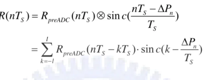
The interfaces of RF and baseband data are digital to analog converter (DAC) in the transmitter and analog to digital converter (ADC) in the receiver side. The oscillators used to generate the DAC and ADC sampling instants at the transmitter and receiver will never have exactly the same period. The ADC is the first stage of baseband, so it dominates the receiving SNR. To get the highest input SNR, the ADC is hoped to sample at the eye open position where it has the maximum signal power. However, the initial sampling phase could be anywhere in the eye diagram, so timing synchronization is necessary. The ADC has two kinds of clock source: free running clock and PLL output clock. With free running clock, this method also called non-synchronous sampling or fix sampling, clock frequency and phase are fixed. Once timing error estimated, the compensation would be performed with interpolator. With PLL output clock, also called synchronous sampling or dynamic sampling, it receives the timing error and adjusts its frequency and phase to compensate the error. There is a need to maintain synchronization while the accuracy and stability of the original clock reference in the receiver may not be ideal. These tasks are the responsibility of a specific module Delay Lock Loop (DLL). Figure 2-12 shows an example of oversampled signal with SCO.

In the MATLAB platform, the model of clock drift is built using the concept of interpolation. The input digital signal and the shifted sinc wave can interpolate the

value between two sampling points. The sampling phase can be written as nTS-ΔPN.

And then we get the ADC output signal R(nTS) by convoluting the ADC input signal

RpreADC(nTS) and shifted sinc wave. The received signal after ADC can be derived as

equation where (2.3) l is the sampling point index.

( ) ( ) sin ( ) ( ) sin ( ) S n S preADC S S l n preADC S S k l S nT P R nT R nT c T P R nT kT c k T =− − Δ = ⊗ Δ =

∑

− ⋅ − (2.3)

SCO brings a slow shift of the symbol timing point, which rotates subcarriers. And a loss of SNR due to ICI generated by the slightly incorrect sampling instants. The shift of sampled phase in time domain will induce the linear phase error in frequency domain. Figure 2-14 shows the frequency domain behavior of SCO model in the system platform. When clock cycle increases, the range of linear phase error will increase.

Chapter 3

Proposed Algorithm

N this chapter, we propose an algorithm to tolerate Wide Clock Offset. The 2*2 MIMO-OFDM system with Wide Clock Offset is aimed. To simplify the problem, we fixed the SCO ppm from 0 to 10000 of thousand multiplier. In the standard of 802.11n , each MIMO OFDM symbol has ten Legacy Short Training Sequences (L-STS) of 16 samples as we mentioned in the section 2.1.3 .To achieve our goal we extend the number of Legacy Short Training Sequences from 10 to 51. The first three short preambles are for packet detection and boundary detection , and the rest of them are for Coarse and Fine timing synchronization of Wide Clock Offset . Figure 3-1 is the scheme of the proposed algorithm. Our algorithm includes Coarse and Fine estimation of SCO. The main goal of Coarse compensation is to bound the residual SCO to the range of SCO from 0 to 3000 ppm of thousand multiplier. After each estimation we’ll send a signal to DAC to compensate the SCO that we estimated.

Received signal Packet detection Boundary detection Coarse Sco estimation & compensation (24 L-STF) Fine Sco estimation& compensation (24 L-STF) Cost 3 L-STF To CFO estimation

Packet Synchronization Timing Synchronization

Figure 3-1 Flowchart of the proposed algorithm

3.1 Coarse timing synchronization of Wide Clock

Offset

In order to estimate SCO of wider scope, we have to find a way to separate the SCO from different quantity. Firstly we try to solve it by the radical ten L-STF. However it’s too few to accumulate the difference between each distinct SCO quantity. We found that we can use much more L-STF to achieve it. So we extend the amount of legacy short preamble from ten to fifty-one. We use twenty-four short preamble to do Coarse SCO estimation and each eight short preambles we define as an Basic unit here. We collect three basic unit with different SCO quantity. Figure 3-2 shows the three basic unit. We control DAC to let the different Basic unit has distinct SCO quantity. Original SCO +6000ppm (4~11th L-STF) Original SCO + 11000ppm (12~19th L-STF) Original SCO +1000ppm (20~27th L-STF)

Basic unit 1 Basic unit 2 Basic unit 3

+5000ppm

-5000ppm

Figure 3-2 The three basic unit of Coarse SCO estimation

The way we will introduced can separate SCO quantity from 6000 to 16000

ppm of thousand multiplier. Because the parameter of R+5000 and R-5000 will have

apparent diversity from 6000 to 16000 ppm of SCO. And that is why we need to add pseudo SCO quantity of 6000 ppm to the Basic unit 1. In order to distinguish SCO from different quantity we let the Basic unit 2 and Basic unit 3 have different SCO quantity as Figure 3-2 illustrated. Basic unit2 and Basic unit 3 both differentiate positive and negative of SCO quantity of 5000 ppm from Basic unit 1. The difference between Basic units of SCO “5000 ppm” is accrued by a great deal of dissimilar

simulation. With this distinct SCO quantity between each Basic unit we can achieve our goal. After the collection of the three Basic units, we can start the Coarse SCO estimation. Since each Basic unit has 8 L-STF so it has 128 points in it. We define Rij as the point of ith Basic unit and jth position. From equation (3-2) (3-3) (3-4) we can get R+5000 , R-5000 , R+－5000diff .

Figure 3-3 R+5000 and R-5000 in each SCO quantity of 10000 packets

1 ( ) ( ) tan ( ) ( ) imag z angle z real z − = (3-1) 96 5000 2 1 1 ( ( j( ) j( ))) j R₊ abs angle R t R t = =

∑

− (3-2) 96 5000 3 1 1 ( ( j( ) j( ))) j R₋ abs angle R t R t = =

∑

− (3-3)

R

+−5000diff

=

R

+5000

−

R

−5000 (3-4)

By the three parameters we can accomplish the coarse SCO estimation. Figure

3-3 is the simulation result of R+5000 and R-5000 from 0 to 10000 SCO ppm of 10000

packets. From this figure we can see that there is evident discrepancy between R+5000

Since we know how to calculate these three parameters , we do some simulation to get them and analysis these simulation results.

The simulation environment below is based on the following conditions: z MIMO-OFDM system in 20 MHz

z packet no. is 10000 z PSDU is 1024 bytes z MCS is 13 SNR is 24

z Decoder using soft Viterbi decoder

z Multipath Model : TGnE (rms delay spread 100 and tap numbers 15) z Decoder using soft Viterbi decoder

Original SCO Value of R+5000 Value of R-5000  Value of R+-5000diff 

0

8.4852≦R+5000≦94.6259 13.861≦R-5000≦64.4957 -29.19≦R+‐5000diff≦79.96

1000

73.8958≦R+5000≦146.36 1. 2780≦R-5000≦58.0144 55.52≦R+‐5000diff≦129.44

2000

131.1874≦R+5000≦185.5 1.6382≦R-5000≦58.6763 108.92≦R+‐5000diff≦182.38

3000

182.9915≦R+5000≦226.2 2. 3877≦R-5000≦47.6644 152.34≦R+‐5000diff≦212.54

4000

201.9628≦R+5000≦251.8 2. 6223≦R-5000≦45.6039 166.46≦R+‐5000diff≦242.22

5000

192.1705≦R+5000≦241.3 2. 4401≦R-5000≦48.1522 155.50≦R+‐5000diff≦235.65

6000

172.3893≦R+5000≦224.2 2. 4665≦R-5000≦54.2802 138.17≦R+‐5000diff≦214.72

7000

135.6931≦R+5000≦197.1 82.6823≦R-5000≦135.635 18.11≦R+‐5000diff≦95.35

8000

131.6822≦R+5000≦195.3 210. 9979≦R-5000≦251.52 -103.71≦R+‐5000diff≦-28.01

9000

139.427≦R+5000≦203.73 278. 0854≦R-5000≦309.71 -157.94≦R+‐5000diff≦ -83.0

10000

144.7336≦R+5000≦213.8 174. 9550≦R-5000≦220.14 -57.04≦R+‐5000diff≦18.11

Decision Condition Est_Sco_coarse 5000

0

<

R

_{+− diff}

<

70

₀

5000

70

<

R

_{+− diff}

<

120

1000

5000

120

<

R

_{+− diff}

<

160

2000

5000

160

<

R

_{+− diff}

<

210

3000

5000

210

<

R

_{+− diff}

4000

5000

80

<

R

₋

<

150

7000

5000

104

R

_{+− diff}

30

−

<

< −

₈₀₀₀

5000

260 R

<

₋

₉₀₀₀

5000

30

R

_{+− diff}

0

−

<

<

₁₀₀₀₀

Table 3-2 Decision criteria of Coarse SCO estimation

Original SCO Estimation result

0 77 errors, 70 packets 10000,7 packets 1000

1000 69 errors, 40 packets 0 , 29 packets 2000

2000 206 errors, 5 packets 1000 , 201 packets 3000

3000 54 errors, 35 packets 2000 , 19 packets 4000

4000 3962 errors, 3962 packets 3000

5000 10000 errors,7 packets 2000 , 8680 packets 3000

1313 packets 4000

6000 10000 errors, 167 packets 4000, 9843 packets 3000

7000 No errors

8000 1 error, 1 packet 10000

9000 No errors

10000 2790 errors, 2740 packets 8000, 50 packets 0

Table 3-1 is the simulation result of R+5000, R-5000 and R+－5000diff in each distinct

SCO quantity of 10000 packets. Each value of these three parameters in each SCO quantity all has a range. After analyzing Table 3-1 we can find out the colored content is useful. There are some overlap between the Table 3-1 even the colored contents. So we must adjust these range of useful value for the good of differentiating SCO from different quantity. Table 3-2 is the result after analyzing and modifying of colored content in Table 3-1. By the value of Table 3-2, it becomes the decision criteria of our coarse SCO estimation. Because when Original SCO equals to 5000 or 6000 ppm, the value of the three parameters will overlap with others. So we can’t tell them from each other. Table 3-3 is the result of Coarse SCO estimation. From this result we can see that when Original SCO equals to 7000 or 9000 ppm , the estimation is perfect without errors. The worse condition is when Original SCO equals to 5000 or 6000 ppm, they will be recognized as the SCO ppm ranging from 2000 to 4000 ppm. Obviously, there may be some Residual SCO exist after our coarse SCO compensation. Residual SCO can be acquired by equation (3-5). The range of the Residual_SCO is almost from 0 to 3000 ppm. The Residual Sco will be compensated after the Fine SCO estimation.

3.2 Fine timing synchronization of Wide Clock

Offset

Residual SCO (28~35th L-STF) Residual SCO + 8000 ppm (36~43th L-STF) Residual SCO – 8000 ppm (44~51th L-STF)

Basic unit 1 Basic unit 2 Basic unit 3

+8000ppm

-8000ppm

Figure 3-4 The three basic unit of fine SCO estimation

Figure 3-4 is the three basic unit of fine SCO estimation. It quiet similar to the figure 3-2. The only difference is that the SCO gap of basic unit 2 and basic unit 3 with basic unit 1 is 8000 ppm but not 5000 ppm. We do much simulation to decide the SCO gap of Coarse and Fine SCO estimation. By equation (3-1) (3-2) (3-3) (3-4) we

can also calculate R+8000 , R-8000 , R+－8000diff three parameters in the same way. Because

the Residual SCO we focused only in the range of 0 to 3000 ppm. So we also show the value of three parameters in these SCO ppm. Figure 3-5 is the simulation result of R+8000 and R-8000 with 10000 packets in the SCO range from 0 to 3000.

Original SCO Value of R+8000 Value of R-8000  Value of R+-8000diff 

0 116.37≦R+8000≦211.00 175.62≦R-8000≦258.28 -101.06≦R+‐8000diff≦0

1000 237.45≦R+8000≦304.54 199.42≦R-8000≦279.58 0≦R+‐8000diff≦70

2000 126.473≦R+8000≦208.94 20.76≦R-8000≦120.05 70≦R+‐8000diff≦176.8608

3000 86.40≦R+8000≦185.24 268.96≦R-8000≦315.06 -215.67≦R+‐8000diff≦-101

Table 3-4 The value of R+8000, R-8000 and R+－_8000diff in each different SCO quantity

Decision Condition Est_Sco_fine

8000

115

R

_{+− diff}

0

−

<

<

₀

8000

0

<

R

_{+− diff}

<

70

₁₀₀₀

8000

70

<

R

_{+− diff}

<

180

2000

8000

215

R

_{+− diff}

115

−

<

< −

₃₀₀₀

Table 3-5 Decision criteria of Fine SCO estimation

Table 3-4 is the value of three parameters with 10000 packets. After

analysis and modification of Table 3-4 we can get new range of the three parameters in Table3-5. The content of Table 3-5 is the criteria of Fine SCO estimation. By the result of Table 3-5 we can start to Fine SCO estimation. Table 3-6 is the simulation

result of Fine SCO estimation with 10000 packets.

Residual SCO

Estimation result

0 3

errors

1000 95

errors

2000 155

errors

3000 10

errors

Table 3-6 Fine SCO estimation of 10000 packets

From Table 3-6 we can see that the result of fine SCO estimation is

acceptable. The error rate of fine SCO estimation is about 1.55% at most. By equation (3-6) we can calculate out the Sco_to_DAC. We’ll alert a control message to the DAC to let the rest data has the SCO quantity of Sco_to_DAC. Obviously , if the Sco_to_DAC equals to zero then the compensation of the SCO will be correct. In the next chapter we’ll show the system performance with our proposed algorithm.

Chapter 4

Simulation result

To evaluate the proposed algorithm, a typical MIMO-OFDM system based on IEEE 802.11 wireless LANs, TGn sync proposal technical specification is used as

a reference-design platform. We chose MATLAB as our simulation language, due to its ability to mathematics, such as matrix operation, numerous math functions, and easily drawing figures as our simulation result to illustrate the performance.

4.1 Simulation Environment

The simulation environment below is based on the following conditions: z MIMO-OFDM system in 20 MHz

z PACK no. is 1000 z PSDU is 1024 bytes z MCS is 13

z Decoder using soft Viterbi decoder

z Random SCO from 0 to 10000 of thousand multiplier

Multipath Model : TGn-E and relative rms delay and Tap number will be shown in table 4-1.And the MCS set will be shown in table 4-2.

Mode

rms delay spread

Tap numbers

A 0

ns 1

B 15

ns 2

C 30

ns 5

D 50

ns 8

E 100

ns 15

F 150

ns 22

Table 4-1 TGn Multipath Specifications

MCS Index Modulatin Antenna No. Code Rate

8 BPSK 2 1/2 9 QPSK 2 1/2 10 QPSK 2 3/4 11 16 QAM 2 1/2 12 16 QAM 2 3/4 13 64 QAM 2 2/3 14 64 QAM 2 3/4 24 BPSK 4 1/2 25 QPSK 4 1/2 26 QPSK 4 3/4 27 16 QAM 4 1/2 28 16 QAM 4 3/4 29 64 QAM 4 2/3 30 64 QAM 4 3/4 Table 4-2 MCS set

4.2 Simulation Result

14 14.5 15 15.5 16 16.5 17 17.5 18 18.5 19 0 0.1 0.2 0.3 0.4 0.5 0.6 0.7 0.8 0.9 1 PER vs SNR SNR(dB) PER Ideal Comp

SCO 10000 ppm with comp SCO 10000 ppm without comp

Figure 4-1 PER VS SNR of ideal and non-ideal situation

10 12 14 16 18 20 0 0.05 0.1 0.15 0.2 0.25 0.3 0.35 Error rate vs SNR SNR(dB) E rror rat e

Error rate of proposed Algorithm

10 12 14 16 18 20 22 24 0 500 1000 1500 2000 2500 RMSE vs SNR SNR(dB) RM S E

RMSE of proposed Algorithm

Figure 4-3 RMSE VS SNR of the proposed algorithm

-10000 0 1000 2000 3000 4000 5000 6000 7000 8000 9000 10000 11000 0.1 0.2 0.3 0.4 0.5 0.6 0.7 0.8 0.9 1

PER of Each SCO ppm in different SNR

SCO(ppm) PE R SNR17 SNR18 SNR19 SNR20 SNR21

(a) (b)

Figure 4-6 Constellation of SCO 1000 ppm under 2x2 MIMO-OFDM system (a) w/o SCO compensation (b)with SCO compensation

Figure 4-7 Constellation of SCO 5000 ppm under 2x2 MIMO-OFDM system (a) w/o SCO compensation (b)with SCO compensation

Figure 4-8 Constellation of SCO 10000 ppm under 2x2 MIMO-OFDM system (a) w/o SCO compensation (b)with SCO compensation

-2 -1.5 -1 -0.5 0 0.5 1 1.5 2 -2 -1.5 -1 -0.5 0 0.5 1 1.5 2 -2 -1.5 -1 -0.5 0 0.5 1 1.5 2 -2 -1.5 -1 -0.5 0 0.5 1 1.5 2 -2 -1.5 -1 -0.5 0 0.5 1 1.5 2 -2 -1.5 -1 -0.5 0 0.5 1 1.5 2 -2 -1.5 -1 -0.5 0 0.5 1 1.5 2 -2 -1.5 -1 -0.5 0 0.5 1 1.5 2 -2 -1.5 -1 -0.5 0 0.5 1 1.5 2 -2 -1.5 -1 -0.5 0 0.5 1 1.5 2 -2 -1.5 -1 -0.5 0 0.5 1 1.5 2 -2 -1.5 -1 -0.5 0 0.5 1 1.5 2

4.3 Simulation analysis

1000 2 1 (Residual_Sco - Est_Sco_Fine) RMSE = 1000 Packet

∑

= (4-1)

From figure 4-1 we can see that the system performance PER will degrade about 0.2 dB with the proposed algorithm. We proposed a novel scheme for the estimation of Wide Clock Offset. From figure 4-2 we can see that the pure error rate of the proposed algorithm is acceptable(less than 8%) when SNR is bigger than 16. This illustrates that we can estimate SCO correctly under SNR 19 dB. Figure 4-3 is the RMSE of the proposed algorithm. From this simulation we can see that the RMSE will converge at SNR 24 dB. This is because all the R value we evaluated is at SNR 24 dB. Figure 4-4 shows the performance in Each SCO ppm with different SNR. We can see that when SNR bigger than 19 the packet error rate will be much closer. Figure 4-6、4-7、4-8 are the constellation of SCO effect of 1000 ppm 、 5000 ppm and 10000 ppm. From this simulation result we can see that the constellation will disperse severely with the SCO ppm turns to be bigger. And after the compensation of our algorithm, we’ll eliminate this phenomenon.

Chapter 5

The Proposed Architecture

The whole architecture can be divided into two main parts, Coarse SCO estimation and Fine SCO estimation. The compensation of SCO only needs to send a signal to DAC to compensate the rest data of estimation result. The most importance of the proposed SCO estimation is to calculate out the three parameters as we mentioned in section 3-1 and 3-2. Since the behavior of the coarse and fine estimation is the same, so we can share the hardware of them.

Figure 5-1 Block diagram of the proposed algorithm

Three parameter

s

generator Estimate SCO

ES T_ SCO MU X MU X MU X Tw o’ s Co mp le m ent Tw o’ s Co mp le m en t 1 (t an )₋ 1 (t an )₋ MUX 10 MU X 10 Bu ffe r Co unt er To 96 B uffe r MU X 10 MUX 10 SCO Es tima tor MUX MU X MU X Tw o’s Co mp lem ent Tw o’s Co mp lem en t 1 (tan) − 1 (tan) − MU X 10 MUX 10 Bu ff er Co un te r To 9 6 Bu ffer MU X 10 MU X 10 SC O Es ti ma to r ES T_ SCO

Chapter 6

Conclusion and Future Work

6.1 Conclusion

In this thesis, a novel Sampling Clock Offset estimation of Wide Scope based on IEEE 802.11n is proposed. This is based on short training field of the preamble. We can combat SCO from 0 to 10000 ppm of thousand multiplier. In order to distinguish the Wide SCO from different quantity we extend the number of L-STF from ten to fifty-one. By this changes we can have good performance on SCO estimation. From the simulation result we can see that the packet error rate degrade about 0.2 dB from the perfect condition. We also can correctly estimate the SCO under SNR 19 dB of the perfect compensation. From the result we can see that our algorithm can tolerate Wide SCO in the presence of AWGN and Multipath. Table 6-1 shows the comparison result of performance in the presence of SCO with other methods. From this table we can see that only our algorithm can tolerate SCO quantity bigger than 1000 ppm.

  Ref [14] Ref [17] Ref [19] Proposed WORK System SISO 2x2 MIMO SISO 2x2 MIMO Modulation 16 QAM N/A OFDM

64 QAM

OFDM 64 QAM

Sampling Method Non-

Synchronous

Non- synchronous

Non-

synchronous Synchronous

Architecture Interpolator Interpolator Interpolator Non-PLL/DLL

(ADCM)

Sampling Rate 1x 1x 4x 1x

Converged Cycle 32 symbols 20 symbols N/A 48 symbols

SCO Range 100 ppm 500 ppm ±200 ppm

0~10000 ppm of thousand

multiplier

6.2 Future work

The proposed algorithm in this thesis can have good performance in the SCO ppm from 0 to 10000 of thousand multiplier as we supposed. So our future work is to tolerate SCO not only those quantity as we mentioned above. Or we can use fewer numbers of short preamble to achieve Wide SCO estimation. The trade-off between cost and performance must be a critical consideration.

Bibliography

[1]ETSI EN 300 401 V1.3.2,”Radio Broadcasting Systems; Digital Audio Broadcasting (DAB) to mobile, portable and fixed receivers”, september 2000.

[2] ETSI EN 301 701 V1.1.1,”Digital Video Broadcasting (DVB); OFDM modulation for microwave digital terrestrial television”, august 2000.

[3] ETSI TS 101 475 V1.2.2,”Broadband Radio Access Networks (BRAN);HIPERLAN Type 2; Physical (PHY) layer”, February 2001

[4] T. Pollet, M. Van Bladel, and M. Moeneclaey, ”BER sensitivity of OFDM systems to carrier frequency offset and Wiener phasenoise,” IEEE Transactions on Communications, vol. 43, pp. 191-193,Feb./Mar./Apr. 1995. P.

[5] T. Pollet, T. Spruyt, and M. Moeneclaey, ”The BER Performance of OFDM Systems Using Non-Synchronized Sampling,” in Proc. IEEE Global Telecomm. Conf (GLOBECOM), Dec. 1994, pp. 253-257.

[6] TGn Sync Group, IEEE P802.11 Wireless LAN - TGn Sync Proposal Technical Specification, Proposal of IEEE802.11n, IEEE Document 802.11-04/889r4.

[7] H. Moose, ”A technique for orthogonal frequency division multiplexing frequency offset correction,” IEEE Tran. on Comm., vol. 42, pp. 2908-2914, Oct. 1994.

[8] T. M. Schmidl and D. C. Fox, ”Robust frequency and timing synchronization for OFDM,” IEEE Transactions on Communications, vol. 45, pp. 1613-1621, Dec. 1997. [9] Z. Zhang, K. Long and Y. Liu, ”Joint frame synchronization and frequency offset estimation in OFDM systems,” IEEE Transactions onBroadcasting, Vol. 51, Sept. 2005.

[10] J.-J. Van de Beek, M. Sandell, and P. O. B‥orjesson, ＂ML estimation of time and frequency offset in OFDM systems,” IEEE Transanctions on Signal Processing, vol. 45, pp. 1800-1805, July 1997.

[11] H. Liu and U. Tureli ,”A high efficiency carrier frequency estimator for OFDM communications,” IEEE Communications Letters, vol. 2, pp. 104-106, Apr. 1998. [12] B. Chen and H. Wang,”Blind estimation of OFDM carrier frequency offset via oversampling,” IEEE Transactions on Signal Processing, vol. 52, issue: 7 , pp. 2047-2057, July 2004.

[13]802.11n standard, ”TGn Sync Proposal Technical Specification”, IEEE 802.11-04/0889r7, July 2005

[14]Muh-Tian Shiue; Chin-Long Wey ,”A non-synchronized sampling scheme ,”May 2006 Page(s):427 - 431 Digital Object Identifier 10.1109/EIT.2006.252124

[15] M. J. Zhao, P. L. Qiu and J. H. Tang, "Sampling rate conversion and symbol timing for OFDM software receiver" IEEE 2002 International conference on

Communications, Circuits and Systems and West Sino Expositions. vol. 1, pp. 114-118, July. 2002.

[16]E. Zhou, X. Zhang and H. Zhao, "Synchronization Algorithms for MIMO OFDM Systems" Wireless Communications and Networking Conference, 2005 IEEE. vol. 1, pp. 18-22, Mar. 2005

[17]Yuanxin Xu, Ling Dong and Cheng Zhang,” Sampling Clock Offset Estimation Algorithm Based on IEEE 802.11n”, Networking, Sensing and Control, 2008. ICNSC 2008. IEEE International Conference on

[18]T. M. Schmidl and D. C. Fox, ”Robust frequency and timing synchronization for OFDM,” IEEE Transactions on Communications, vol. 45, pp. 1613-1621, Dec. 1997. [19]E. Oswald,” NDA based feed forward sampling frequency synchronization for OFDM systems ,”in IEEE Vehicular Technology Conference, pp. 1068-1072, 2004