小型化洩漏波天線與雙頻圓極化槽狀單極天線

國 立 交 通 大 學

電信工程研究所

碩 士 論 文

小型化洩漏波天線與雙頻圓極化槽狀單極天線

Compact Leaky-Wave Antenna and

Dual-band Circularly Polarized Slotted Monopole Antenna

研 究 生：黃建榮 (Chien-Rung Huang)

指導教授：周復芳 博士 (Dr. Christina F. Jou)

小型化洩漏波天線與雙頻圓極化槽狀單極天線

Compact Leaky-Wave Antenna and

Dual-band Circularly Polarized Slotted Monopole Antenna

研究生：黃建榮 Student：Chien-Rung Huang 指導教授：周復芳 博士 Advisor：Dr. Christina F. Jou

國 立 交 通 大 學

電信工程研究所

碩士論文

A Thesis

Submitted to Department of Computer and Information Science College of Electrical Engineering and Computer Engineering

National Chiao Tung University in partial Fulfillment of the Requirements

for the Degree of Master of Science In Communication Engineering

June 2012

Hsinchu, Taiwan, Republic of China

小型化洩漏波天線與雙頻圓極化槽狀單極天線

研究生：黃建榮

指導教授：周復芳

博士

國立交通大學

電信工程研究所

碩士班

中文摘要

本論文主要包含二大部份：1.

利用開放式環形諧振器來抑制洩漏

波天線的旁波瓣；2.

利用槽狀結構使單極天線產生雙頻帶且具有圓極

化。在第一部分中，提出二種可以有效抑制旁波瓣的架構，第一種架

構是將開放式環形諧振器放在天線主體的開路端，利用開放式環形諧

振器所產生的截止頻帶效果，使得反射波在此截止頻帶內得以被抑制；

而第二種則是將開放式環形諧振器放在接地金屬的部分，利用此架構

將反射波耦合至開放式環形諧振器，透過此時環形諧振器所產生的截

止頻帶，進而抑制洩漏波天線的反射波。由此可發現，利用開放式環

形諧振器所產生的截止頻帶，不僅僅可以有效地抑制旁波瓣，更可以

減少洩漏波天線的長度，達到縮小化的目的。

在第二部分中，介紹利用槽孔結構產生雙頻帶且圓極化的單極天

線，天線主要架構為螺旋結構，並在其後端接一個圓形的金屬架構；

而在接地金屬中，蝕刻出一個 L 型的槽狀孔，此 L 形的槽孔扮演著

非常重要的角色，不僅可使單極天線能在低頻與高頻的部分產生雙頻

圓極化的效果，更可以調整 L 形的長寬比來選擇雙頻圓極化所要操作

的頻帶。另外，在天線的主體上也再蝕刻二個槽孔結構，此二個槽孔

結構是調整高頻段圓極化操作頻帶的主要因素之一。由此可知，利用

簡單的槽狀結構，亦可使得單極天線產生圓極化的效果。

Compact Leaky-Wave Antenna and Dual-band

Circularly Polarized Slotted Monopole Antenna

Student：Chien-Rung Huang Advisor：Dr. Christina F. Jou

Institute of Communications Engineering

College of Electrical and Computer Engineering

National Chiao Tung University

ABSTRACT

This thesis consists of two parts：1. Using split ring resonators to

suppress the side-lobe level of the tapered compact leaky wave antenna.

And 2. Using the structures of slots to excite dual-band circularly

polarization in monopole antenna. In the first part, we demonstrate two

types of suppressing the reflection wave of the leaky wave antenna. The

first structure is to put the split ring resonators at the open end of the

leaky wave antenna, and the split ring resonators can generate stop-band

to suppress the side-lobe level efficiently. The second structure is to etch

the split ring resonators in the ground plane, and the reflected wave will

couple to the split ring resonators and be trapped. Thus it can be seen that

we can use split ring resonators not only to suppress the side-lobe but also

to reduce the length of the leaky wave antenna.

In the second part, a dual-band circularly polarized monopole

antenna using structures of slots will be introduced. The main structure of

the monopole antenna is a circular strip and we add a circular patch at the

end of the strip. In the ground plane, we etch a L-shaped slot, and this slot

play an important role of exciting the circular polarization not only at the

lower band but also at the upper band. The most important is that we can

choose the different length of the L-shaped slot to operate on the

frequency band what we want. On the other hand, we also add two

notches at the antenna, and these two notches can adjust the operating

frequency band of circular polarization at the upper band. From the above,

we can use these simple structures to get circular polarizations.

誌謝

時間過得飛快，短暫的碩班生活在教授、學長、同學，以及學弟妹的點綴之 下，都變得充實了。謝謝大家的陪伴，在我迷失方向時指引我走向出口。之所以 能夠進入９１９這個大家庭，首先我必須感謝我的指導教授—周復芳教授，感謝 教授在這二年之中悉心的指導與鼓勵，讓剛進入碩士的我有了目標與方向，忘不 了那一天老師在實驗室對我們新生所說的鼓勵的話，謝謝老師！再來，感謝實驗 室的學長們，感謝超舜、玠瑝（Double）、宜星（爽哥）、智鵬，謝謝你們在研究 上的指導與提醒，讓我的研究可以如此順利；還記得我們再趕 APMC 截稿前幾 周的半夜，一群人窩在實驗室玩桌遊，那段時光真的令人難忘，謝謝大家的陪伴。 另外，也不得不提到陪伴我們到澳洲發表論文的玠瑝學長，有學長的陪伴讓我們 的心情輕鬆了不少，這段澳洲之旅也將會是碩班期間難忘的一段回憶！ 我也要感謝陪伴我一起走過２年碩班生活的同學們，易懋、星翰（小賴）、 家宏（阿牟），謝謝你們的陪伴，讓這２年的生活精采了不少，也增添了不少歡 樂；我永遠也忘不了我們一起到澳洲發表成果的這段時光，還記得我們光著腳走 在 BONDI BEACH 的足跡，謝謝易懋、小賴。感謝實驗室的學弟妹們，佑祥 （momo）、雨翔、寶國（阿國）、瑜秀（高手）、玠倫（阿倫）、涵婷（8 妹）以 及馮盛，有你們在的每一天，實驗室都熱鬧無比，謝謝你們！ 另外，我一定要感謝如來實證社的各位，感恩你們大家，真正的感恩與祝福 是無法言喻的，我們有祂的陪伴真的是太棒了！我也要感謝我的女朋友，謝謝妳 容忍我、關心我、陪伴我走過了這 9 年，這段期間很感謝妳陪著我東奔西跑，辛 苦妳了，也感謝妳在我失落的時候默默的護持我，謝謝妳的付出！最後，我要感 謝我的父、母親以及家人們，謝謝你們養育我、教導我、鼓勵我、愛我。最後， 僅將我最微薄也最用心的成果獻給你們。我們一定要一起回到天父的家！ 黃建榮 於風城 交通大學 2012.6

T

ABLES OF

C

ONTENTS

中文摘要 ... i

ABSTRACT ... iii

誌謝 ... v

TABLES OF CONTENTS ... vi

LIST OF FIGURES ... viii

LIST OF TABLES ... xii

CHAPTER 1 INTRODUCTION ... 1

1.1MOTIVATION ... 1

1.2ORGANIZATION ... 2

CHAPTER 2 USING SPLIT RING RESONATORS TO SUPPRESS THE SIDE LOBE AND MINIATURIZE THE LENGTH OF A TAPERED LEAKY WAVE ANTENNA ... 3

2.1BASIC THEORIES ... 4

2.1.1 Theories of leaky wave antenna... 4

2.1.2 Theories of tapering method ... 8

2.1.2 Theories of split ring resonators ... 10

2.2DESIGN OF THE PROPOSED LEAKY WAVE ANTENNA WITH DIFFERENT POSITION OF SPLIT RING RESONATORS ... 12

2.2.1 The influence of the split ring resonators ... 12

2.2.2 First structure - split ring resonator at the end of the antenna ... 15

2.2.3 Second structure - split ring resonator at the end of the ground ... 17

2.3SIMULATION AND MEASUREMENT... 19

2.3.1 Simulations between the prototype and the tapered LWA ... 19

2.3.2 Simulation and measurement of the second structure ... 30

2.4CONCLUSIONS ... 37

CHAPTER 3 A DUAL-BAND CIRCULARLY POLARIZED SLOTTED MONOPOLE ANTENNA ... 38

3.1BASIC THEORIES OF MONOPOLE ANTENNA AND POLARIZATION ... 39

3.1.1 Theories of monopole antennas ... 39

3.1.2 Theories of polarization ... 41

3.2DESIGN OF THE DUAL-BAND CIRCULARLY POLARIZED SLOTTED MONOPOLE ANTENNA ... 43

3.3PARAMETRIC STUDIES ... 45

3.3.1 The influence of the L-shaped slot on the ground layer ... 45

3.3.2 The influences of the two notches on the top layer ... 49

3.4SIMULATION AND MEASUREMENT... 53

3.5CONCLUSIONS ... 59

CHAPTER 4 FUTURE WORKS ... 60

L

IST OF

F

IGURES

Figure 2-1. The electric field distribution of the first higher order mode of the micro-strip line.[5] ... 6

Figure 2-2. Normalized complex propagation constant for the first higher order mode in the micro-strip line with split ring resonators at the antenna. ... 6

Figure 2-3. The coordinate system of a leaky wave antenna. ... 7

Figure 2-4. Three structures of tapered leaky wave antenna [7, 8]. ... 9

Figure 2-5. (a) SRR produced by Pendry and (b) CSRR.[10] ... 11

Figure 2-6. Equivalent circuit model of SRRs.[12] ... 11

(a) Single SRR configuration. (b) Double SRR configuration. ... 11

Figure 2-7. The electric and magnetic field intensity in the transmission line and the transmission line with the SRRs. ... 13

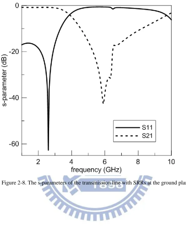
Figure 2-8. The s-parameters of the transmission line with SRRs at the ground plane. ... 14

Figure 2-9. The first structure of the leaky wave antenna. ... 15

Figure 2-10. Configuration of the proposed leaky wave antenna. ... 16

Figure 2-11. The second structure of the leaky wave antenna. ... 17

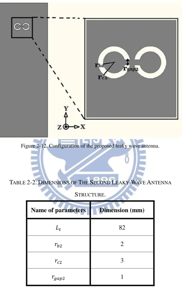
Figure 2-12. Configuration of the proposed leaky wave antenna. ... 18

Figure 2-13. The two structures: (a) prototype, (b) tapered LWA. ... 20

Figure 2-14. Simulated radiation pattern of the prototype and tapered LWA at 4.3GHz ... 21

Figure 2-15. Simulated radiation pattern of the prototype and tapered LWA at 4.5GHz ... 21

Figure 2-16. Simulated radiation pattern of the prototype and tapered LWA at 4.7GHz ... 22

Figure 2-18. The different operating frequency of the first structure. LWA operates at : (a) 4.3GHz ,(b)

4.5GHz, (c) 4.7GHz, (d) 4.9GHz. ... 24

Figure 2-19. Normalized complex propagation constant for the first higher order mode in the micro-strip line with split ring resonators at the antenna. ... 25

Figure 2-20. The measured and simulated return loss of the first structure. ... 26

Figure 2-21. Simulated and measured normalized radiation pattern at 4.3GHz. ... 26

Figure 2-22. Simulated and measured normalized radiation pattern at 4.5GHz. ... 27

Figure 2-23. Simulated and measured normalized radiation pattern at 4.7GHz. ... 27

Figure 2-24. Simulated and measured normalized radiation pattern at 4.9GHz. ... 28

Figure 2-25. Measured normalized radiation patterns of the first LWA structure. ... 28

Figure 2-26. Simulated and measured radiation angle of main beam of the first LWA. ... 29

Figure 2-27. Simulated and measured radiation gain of main beam of the first LWA. ... 29

Figure 2-28. The different operating frequency of the second structure. LWA operates at : (a) 4.3GHz ,(b) 4.5GHz, (c) 4.7GHz, (d) 4.9GHz. ... 31

Figure 2-29. Normalized complex propagation constant for the first higher order mode in the micro-strip line with split ring resonators at the ground plane. ... 32

Figure 2-30. The measured and simulated return loss of the second structure. ... 33

Figure 2-31. Simulated and measured normalized radiation pattern at 4.3GHz. ... 33

Figure 2-32. Simulated and measured normalized radiation pattern at 4.5GHz. ... 34

Figure 2-33. Simulated and measured normalized radiation pattern at 4.7GHz. ... 34

Figure 2-34. Simulated and measured normalized radiation pattern. at 4.9GHz ... 35

Figure 2-36. Simulated and measured radiation angle of main beam of second LWA. ... 36

Figure 2-37. Simulated and measured radiation gain of main beam of second LWA. ... 36

Figure 3-1. Current distribution of a (a)dipole antenna, and (b) monopole antenna.[21] ... 40

Figure 3-2. The geometry of the proposed slot antenna: (a) top layer, (b) ground layer. ... 44

Figure 3-3. The simulated return loss of the conventional and L-shaped slot antenna. ... 46

Figure 3-4. The simulated axial ratio of the conventional and L-shaped slot antenna. ... 46

Figure 3-5. The return loss versus frequency at different 𝑳𝟓. ... 47

Figure 3-6. The axial ratio versus lower-band frequency at different 𝑳𝟓. ... 47

Figure 3-7. The axial ratio versus higher band frequency at different 𝑳𝟓. ... 48

Figure 3-8. Comparison the simulated return loss of adding 2 notches. ... 50

Figure 3-9. Comparison the simulated axial ratio of adding the 2 notches. ... 50

Figure 3-10. The return loss versus frequency at different 𝑾𝟏 ... 51

Figure 3-11. The axial ratio versus lower-band frequency at different 𝑾𝟏 ... 51

Figure 3-12. The axial ratio versus higher-band frequency at different 𝑾𝟏 ... 52

Figure 3-13. Measured and simulated return loss. ... 54

Figure 3-14. Measured and simulated axial ratio at lower frequency band. ... 54

Figure 3-15. Measured and simulated axial ratio at lower frequency band. ... 55

Figure 3-16. The normalized 2.45GHz LHCP radiation pattern. ... 56

Figure 3-17. The normalized 2.45GHz RHCP radiation pattern... 56

Figure 3-18. The normalized 5.2GHz LHCP radiation pattern. ... 57

Figure 3-20. The measured LHCP and RHCP at 2.45GHz ... 58 Figure 3-21. The measured LHCP and RHCP at 5.2GHz ... 58

L

IST OF

T

ABLES

Table 2-1. Dimensions of The First Leaky-Wave Antenna Structure. ... 16

Table 2-2. Dimensions of The Second Leaky-Wave Antenna Structure. ... 18

Table 2-3. The comparisons of the two structures. ... 37

TABLE 3-1. Final Dimensions of Parameters ... 44

C

HAPTER

1

I

NTRODUCTION

1.1 Motivation

In this thesis, there are two topics presented. The first topic has two structures. The first structure is the leaky wave antenna (LWA) with tapered micro-strip line and split ring resonators at the end of the antenna to reduce the size and the side lobe of the LWAs. This research includes the studies of tapering the length of leaky wave antenna and suppressing side lobes. The second structure is that putting the split ring resonators used in the first structure to the end of the ground. The purposed of the second structure is also to achieve the goal of reducing the length and the side lobe of the proposed antenna.

Since 1979, the micro-strip leaky wave antenna (LWA) has been studied and used in many applications such as cruise control and automobile radar system, because of its attractive properties like the beam-scanning capability, low profile, easy fabrication and ease of analysis by the multimode cavity model. The first leaky wave antenna introduced by Menzel[1, 2], much progress has been made regarding the development of leaky wave antennas based on the higher order mode of micro-strip.

The micro-strip leaky wave antenna operates in the first higher order mode 𝑇𝐸₀₁, and the power leaks in the form of space wave. When micro-strip leaky wave antenna works in the leaky band, the power radiates out along its length. A tapered micro-strip leaky wave antenna whose each steps can irradiate in subsequent ranges of frequency is a possible first solution studied to obtain a broadband and fixed main-beam leaky wave antenna.

The second topic is a dual-band circularly polarized slotted monopole antenna. This antenna can be excited a left-hand circular polarization (LHCP) at 2.45GHz, and right-hand circular polarization (RHCP) at 5.2GHz.

Nowadays, antenna with circular polarization plays an important role in communication systems, because they allow for more flexibility in orientation angle between transmitter and receiver antennas, high penetration, and stability. Therefore, circular polarization antennas can provide much better connectivity with fixed and mobile communication systems.

In order to have a circular polarized radiation, the orthogonal field components should have the equal magnitude and a phase difference of 90˚. It is not easy to satisfy the conditions of generating a circular polarization. In recently, slots are widely used in micro-strip antenna designs. The geometry structures of the slots are corresponding to the radiation patterns. It’s known that the spiral structure can achieve circular polarization characteristics.

1.2 Organization

This thesis will begin with the introduction of the leaky wave antenna and some relating theories and techniques in order to facilitate the later analysis. The following chapters will focus on the proposed antenna design.

Chapter 1 gives the brief introduction and the motivation of this paper. Fundamental theories and properties of the micro-strip leaky wave antennas will be summarized in chapter 2. And then, chapter 3 will be demonstrated the design and the operating process of the dual-band circularly polarized slotted monopole antenna. And finally, the future works will be made in the chapter 4.

C

HAPTER

2

U

SING SPLIT RING RESONATORS TO

SUPPRESS THE SIDE LOBE AND

MINIATURIZE THE LENGTH OF A

TAPERED LEAKY WAVE ANTENNA

In this chapter, we will first give a simple introduction on the characteristic of the leaky wave antenna. Second, we will discuss the basic theories and the radiation characteristics of the micro-strip leaky wave antenna. Furthermore, we will also mention the theories of the tapering method and the split ring resonators. Finally, we will give a competition between the different positions of the split ring resonators. By adding split ring resonators on the tapered antenna or on the ground, the current distribution of this antenna can be improved. Besides, the split ring resonators can trap the reflection current which generates the reflection wave. Because of the reducing reflection wave, the side-lobe can also be reduced. This technique not only suppresses the side-lobe but miniaturizes the length of the antenna. According to the measured results of the split ring resonators on the antenna, the impedance bandwidth achieves about 600MHz for 6-dB return loss, which covers the range from 3.4GHz to 4.9GHz, and the scanning angle of the measured main beam is about 31˚, which covers the range from 14˚ to 45˚. In the other case of the split ring resonators on the ground, the measured results show the impedance bandwidth covers from 4.4GHz to 5.0GHz, whose impedance bandwidth achieves about 600MHz for 6-dB return loss.

2.1 Basic theories

2.1.1 Theories of leaky wave antenna

The first prototype of micro-strip leaky wave antenna is presented by Menzel[1] in 1979, which used an asymmetric feed line to excite the first higher order mode. Because the leaky wave antenna is operated in the first higher order mode, and the width of the leaky wave antenna, the thickness of the substrate, and the dielectric constant determines the radiation bandwidth.

Leaky wave antenna uses an asymmetric feed line to excite the first higher order mode (𝑇𝐸₀₁, 𝑙𝑒𝑎𝑘𝑦 𝑚𝑜𝑑𝑒). Generally speaking, the radiation mode of antenna is the dominant mode, which is a slow wave relative to radiating in free space. Comparing to the dominant mode, the first higher mode is a fast wave and excites the characteristics of narrow beam-width and frequency scanning. Figure 2-1 shows the electric and magnetic fields of the first higher order mode, which the electric field is an odd symmetric about the axial centerline and excites a traveling wave.

The theories and the phenomenon of leaky wave antenna had been clearly introduced by Oliner and Lee[2, 3]. For leaky wave antennas, we expect that only leaky mode could exist in the propagation which contributes the leakage radiation. Now we can model this as a lossy transmission line characterized by a complex propagation constant

𝑘𝑦 = 𝛽𝑦− 𝑗𝛼𝑦 (2.1)

, where 𝛽_𝑦 and 𝛼_𝑦 are the phase constant and attenuation constant, respectively. The variation of the normalized phase constant and attenuation constant are plotted in Figure 2-2.

According to Figure 2-2, we divide the first higher order mode into four regions: (1) 𝛼_𝑦 > 𝛽_𝑦, ---> reactive cutoff region,

(2) 𝛽_𝑦 > 𝛼_𝑦, 𝛽_𝑦 < 𝑘₀, ----> surface wave and space wave leakage region, (3) 𝑘_𝑠 > 𝛽_𝑦 > 𝑘₀, ---> surface leakage region,

(4) 𝛽_𝑦 > 𝑘_𝑠, ---> bound mode region;

where 𝑘_𝑠 and 𝑘₀ are the surface wave number and wave number of free space, respectively. From above, when we operate in the (1) region, the mode can’t be constructed, and a large reflection could be expected if an incident wave generated. But when the operating frequency gets larger enough to build up the mode, since the mode is now dominated by fast wave and the wave leads to leak and radiate from the edge of the micro-strip line. When we increase the frequency continuously, the wave may eventually become a slow wave and then there is no space wave radiation[4]. The frequency range we can use for leaky wave antennas falls in the space wave leakage region, which we can simply determine the range between the lower edge (𝑓_𝐿) and the upper edge (𝑓𝐻):

𝛼_𝑦(𝑓_𝐿) = 𝛽_𝑦(𝑓_𝐿) (2.2) 𝛽𝑦(𝑓𝐻) = 𝑘0 (2.3)

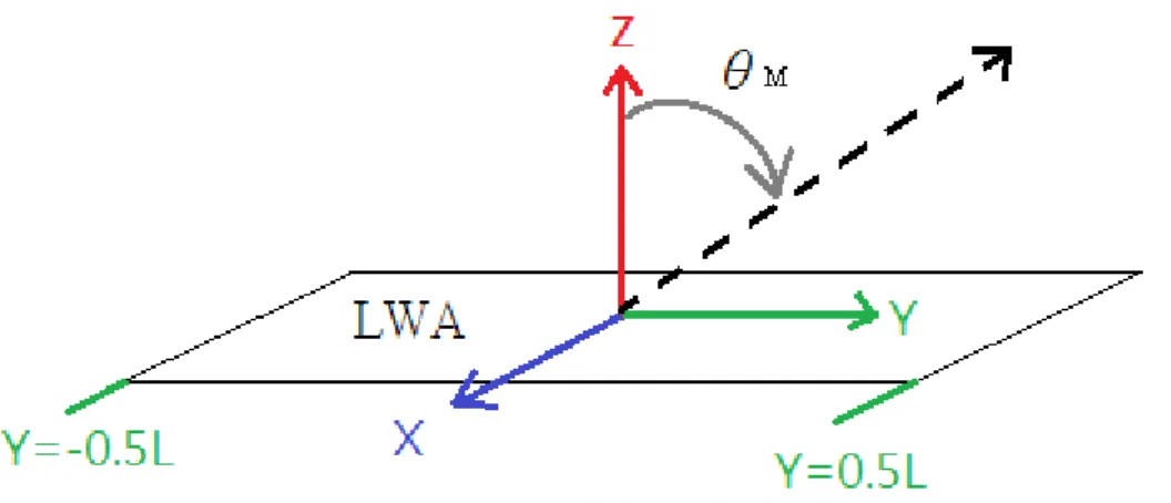
This “lossy transmission line” can be regarded as an antenna which can radiate toward a specific direction, and the direction is dependent on the specific phase constant of the different frequency of the lossy transmission line. Moreover, in Figure 2-3, the elevation angle 𝜃_𝑀 between the main-beam direction and end-fire direction (the Z-axis direction) can be estimated approximately as following equation:

𝜃𝑀 ≅ sin−1(𝛽𝑦⁄ ) (2.4) 𝑘0 𝛼𝑦

𝑘0 ≅ 0.183 × 𝜃𝐻𝑃𝐵𝑊 × cos(𝜃𝑀) (2.5)

Figure 2-1. The electric field distribution of the first higher order mode of the micro-strip line.[5]

Figure 2-2. Normalized complex propagation constant for the first higher order mode in the micro-strip line with split ring resonators at the antenna.

2.1.2 Theories of tapering method

In order to improve the radiation bandwidth, some researches choose the method of tapering. A tapered leaky wave antenna operates by using sections with different width to excite different operating frequency bands, so the tapered leaky wave antenna can achieve broad impedance bandwidth[6, 7]. Although we can increase the impedance bandwidth by tapering the micro-strip line, the problem with tapered leaky wave antenna is that there is a spurious side-lobe generated by the reflection wave. The theory of tapered leaky wave antenna is that the wider width of leaky wave antenna radiates in the lower frequency region and the narrow width acts in the reactive region and not radiates power. Similarly, the narrower width radiates in the higher frequency region and the wider width operates in the bound mode region. The width of the tapered leaky wave antenna can be determined by the start and the end frequency. The equations of the radiation region and cutoff frequency (𝑓_𝑐) of each section is expressed as[8]

𝑓_𝑐 = _2𝑤 𝑐

𝑒𝑓𝑓√𝜀𝑟 (2.6)

𝑓𝑐 < 𝑓 <_√𝜀𝑓𝑐√𝜀𝑟

𝑟−1 (2.7)

where c is the speed of light in the air, 𝑤_𝑒𝑓𝑓 is the effective width of strip line, and 𝜀𝑟 is the dielectric constant of substrate. Figure 2-4 shows three types of tapered

leaky wave antenna. Due to the impedance mismatch and the discontinuity effect caused by the original tapered leaky wave antenna (TYPE 1), the following structures (TYPE 2 and TYPE 3) are fabricated to solve and improve the bandwidth.

2.1.2 Theories of split ring resonators

Because of the significant growing of the communication technology and wireless communication market, consumers’ requirements about the circuits have been trending to be smaller, more reliable and more power efficient[9]. To integrate the whole transceivers on a single chip is the trend for future wireless systems. First of all, we should consider the largest components of the integrated circuit, and it is an important target for wireless communication systems to achieve the miniaturization of antennas[10] .

In recent years, split ring resonators (SRRs) shown in Figure 2-5 (a), proposed by Pendry[10-12], have played a main role of the miniaturization and compatibility in the planar circuits. Because of the characteristics of the negative permeability and permittivity, split ring resonators have attracted a great interest in the circuit and antenna design. Besides, we need to have periodic structures which will not only be easy to fabricate but also will not increase the dimensions of the devices[10].

Split ring resonators are one of the electromagnetic metamaterials (MTMs) which are broadly called left-handed(LH) structures[12]. LH materials are characterized by antiparallel phase and group velocities, or negative relative permittivity and permeability(𝜀𝑟 , 𝜇𝑟 < 0).

A split ring resonator provides a stop-band phenomenon and a negative permeability around the resonant frequency[13, 14]. This MTM exhibits a plasmonic-type permeability frequency function of the form[12]:

𝜇𝑟(𝜔) = 1 − 𝐹𝜔 2 𝜔2_−𝜔 0𝑚 2 _{+𝑗𝜔𝜁} (2.8) = 1 − 𝐹𝜔 2_(𝜔2_−𝜔 0𝑚2 ) (𝜔2_−𝜔 0𝑚 2 ₎2_+(𝜔𝜁)2+ 𝑗 𝐹𝜔2_𝜁 (𝜔2_−𝜔 0𝑚 2 ₎2_+(𝜔𝜁)2 ,

where 𝐹 = 𝜋(𝑎 𝑝⁄ )2 (a : the inner radius of the smaller ring), 𝜔_0𝑚 = 𝑐√_{𝜋 ln(2𝜔𝑎}3𝑝 _{3 𝛿}

⁄ )

( ω : width of the rings, δ : radial spacing between the rings), and ζ = 2𝑝𝑅′ 𝑎𝜇⁄ ₀ (𝑅′_{: the metal resistance per unit length). Equation (2.8) reveals that a}

frequency range can exist:

𝜇_𝑟 < 0, for 𝜔_0𝑚 < 𝜔 < 𝜔0𝑚

√1−𝐹= 𝜔𝑝𝑚 , (2.9)

where the 𝜔_𝑝𝑚 is called the magnetic plasma frequency. The equivalent circuit of a SRR is shown in Figure 2-6. In the single SRR, the circuit model is the RLC resonator with resonant frequency 𝜔₀ = 1 √𝐿𝐶⁄ .

Figure 2-5. (a) SRR produced by Pendry and (b) CSRR.[10]

Figure 2-6. Equivalent circuit model of SRRs.[12] (a) Single SRR configuration. (b) Double SRR configuration.

2.2 Design of the proposed leaky wave antenna with

different position of split ring resonators

2.2.1 The influence of the split ring resonators

From [12, 13], we can know that the split ring resonators generate an important phenomenon called stop-band which can forbid the wave to pass through. In order to finding the difference between the transmission line with and without the split ring resonators, the following simulation shown in Figure 2-7 can tell us the influence of the split ring resonators.

In this section, we focus on the influence of the split ring resonators. First of all, comparing the simulation between the transmission line and the transmission line with split ring resonators, and we can easily find out that the electric field and magnetic field are trapped by the split ring resonators which are shown in Figure 2-7.

In other words, the split ring resonators will reduce the reflection wave of the open end side of the leaky wave antenna when the split ring resonators are operating at the stop-band. According to this phenomenon, we can choose the split ring resonators not only to suppress the reflection wave but also to reduce the size of leaky wave antenna. From Figure 2-8, we can know that the resonant frequency of the transmission line starts to resonate from 4GHz to 9.5GHz.

From these simulations, we can know that we must choose the right position of the split ring resonators. Our purpose is to reduce the side-lobe, so we have to put the split ring resonators at the end of the antenna.

Figure 2-7. The electric and magnetic field intensity in the transmission line and the transmission line with the SRRs.

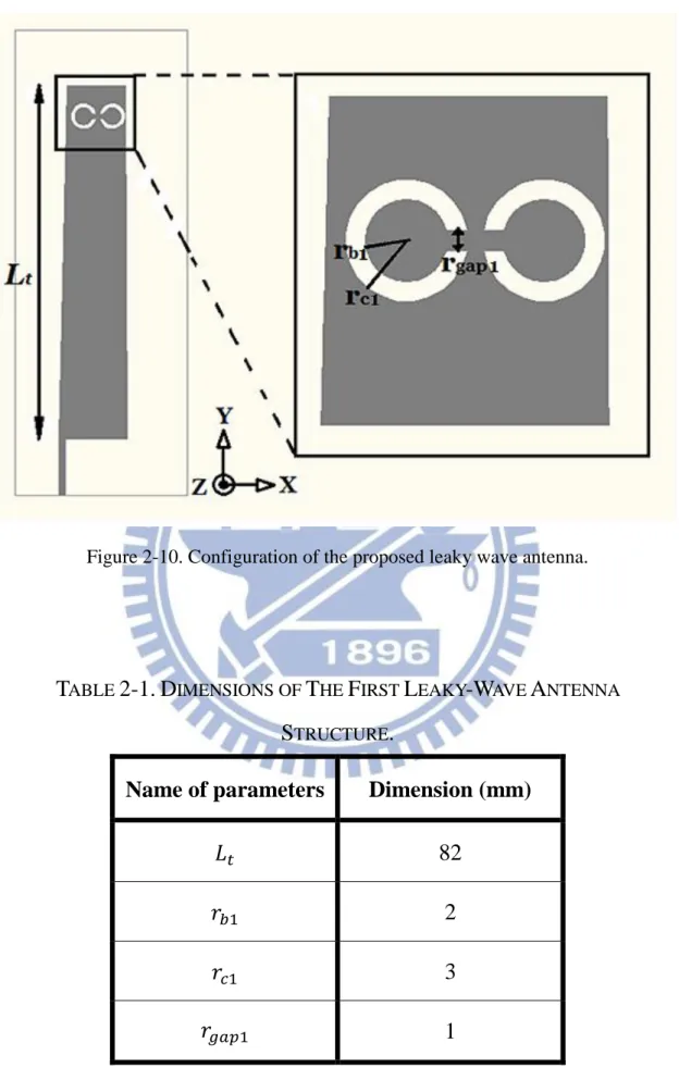
2.2.2 First structure - split ring resonator at the end of the antenna

Figure 2-10 shows the proposed configuration of the leaky wave antenna. This antenna is fabricated on FR4 substrate with a dielectric constant (𝜀_𝑟) of 4.4, loss tangent (tan 𝛿) of 0.024, and thickness of 0.8mm. The total length (𝐿𝑡) of the tapered

short leaky wave antenna is chosen to be 82mm (about 1.18𝜆₀ at 4.3GHz). The radius of each ring and the other antenna parameter are listed in Table 2-1.

In this section, the design procedures of this antenna, including the etched split ring resonators on the antenna for suppressing the reflection wave, are presented sequentially.

Figure 2-10. Configuration of the proposed leaky wave antenna.

T

ABLE

2-1.

D

IMENSIONS OF

T

HE

F

IRST

L

EAKY

-W

AVE

A

NTENNA

S

TRUCTURE

.

Name of parameters

Dimension (mm)

𝐿

_𝑡

82

𝑟

_𝑏1

2

𝑟

_𝑐1

3

2.2.3 Second structure - split ring resonator at the end of the ground

Figure 2-12 shows the proposed configuration of the leaky wave antenna. This antenna is also fabricated on FR4 substrate with thickness of 0.8mm. The total length (𝐿𝑡) of the tapered short leaky wave antenna is chosen to be 82mm (about 1.18𝜆0 at

4.3GHz). The radius of each ring and the other antenna parameter are the same as the first structure.

In this section, the design procedures of this antenna, including the etched split ring resonators on the ground for suppressing the reflection wave, are presented sequentially.

Figure 2-12. Configuration of the proposed leaky wave antenna.

T

ABLE

2-2.

D

IMENSIONS OF

T

HE

S

ECOND

L

EAKY

-W

AVE

A

NTENNA

S

TRUCTURE

.

Name of parameters

Dimension (mm)

𝐿

_𝑡

82

𝑟

_𝑏2

2

𝑟

_𝑐2

3

2.3 Simulation and measurement

2.3.1 Simulations between the prototype and the tapered LWA

In this section, we take the first step to check the difference between the prototype and the tapered leaky wave antenna. In order to figure out the influence of the tapering method using on the leaky wave antenna, we use the simulation tools(HFSS) to check the differences. First, we make the length (Lt) of the prototype LWA which is shown in Figure 2-13 to be 82mm which is about 1.18𝜆₀ at 4.3GHz. And for the second step, we use the HFSS to make sure that the tapering method also suppresses the side-lobe of the LWA.

From Figure 2-14 to Figure 2-17 show the comparison of the radiation patterns between the prototype and the tapered leaky wave antenna. We can notice that the orientation of the main beam seems tilt toward broad side, because the proposed tapering reduces the width and make the phase constant be reduced in the same frequency point. From Eq(2.4), we can expect that tapering method can lead the beam to toward the broadside. It can be seen that the side lobes are suppressed due to the tapering method in the scanning range (from 4.3GHz to 4.9GHz). Moreover, we can know that the side-lobe is suppressed efficiently by more than 20dB in the 4.3GHz and 4.5GHz which are shown in Figure 2-14 and Figure 2-15. And for 4.7GHz and 4.9GHz, the side lobe levels are approximately suppressed by 9dB and 5dB, respectively.

Figure 2-14. Simulated radiation pattern of the prototype and tapered LWA at 4.3GHz

Figure 2-16. Simulated radiation pattern of the prototype and tapered LWA at 4.7GHz

2.3.2 Simulation and measurement of the first structure

In this section, we take the first step to verify that whether the split ring resonators work or not. From the simulation shown in Figure 2-18, we can know that the reflecting wave from the open end can be gathered by the split ring resonators, so it won’t be radiated to the air. Due to the results from these simulations, we can verify that the position of the split ring resonators should be put at the open end which generating reflecting waves.

The simulated normalized phase constant and attenuation constant are shown in Figure 2-19, and the usable range is approximately from 4.3GHz to 4.9GHz. From Figure 2-20, we can see the simulated and measured return loss of the first structure of leaky wave antenna. The measured impedance bandwidth of the first leaky wave antenna for 6-dB return loss is approximately from 4.3GHz to 4.9GHz, and it has good agreement between the simulation and the measurement. And then, from Figure 2-21 to Figure 2-25, they show the simulated and measured normalized radiation patterns in the Y-Z plane, and finally illustrate the measured radiation pattern at each operating frequency: 4.3GHz, 4.5GHz, 4.7GHz, and 4.9GHz. And from the radiation patterns, we can find that the scanning degree is nearly from 10˚ to 45˚ of the first structure of the leaky wave antenna. The simulated and measured maximum gain and radiation angle are also shown in Figure 2-26 and Figure 2-27, respectively.

Figure 2-18. The different operating frequency of the first structure. LWA operates at : (a) 4.3GHz ,(b) 4.5GHz, (c) 4.7GHz, (d) 4.9GHz.

Figure 2-19. Normalized complex propagation constant for the first higher order mode in the micro-strip line with split ring resonators at the antenna.

Figure 2-20. The measured and simulated return loss of the first structure.

Figure 2-22. Simulated and measured normalized radiation pattern at 4.5GHz.

Figure 2-24. Simulated and measured normalized radiation pattern at 4.9GHz.

Figure 2-26. Simulated and measured radiation angle of main beam of the first LWA.

2.3.2 Simulation and measurement of the second structure

In this part, we focus on the same structure but put the split ring resonators at the ground plane. In the second structure, the first verification is to check the simulation results whether the structure works or not. From Figure 2-28, we know that the reflecting wave is also trapped by the split ring resonators.

The simulated normalized phase constant and attenuation constant are shown in Figure 2-29, and the usable range is approximately from 4.3GHz to 4.9GHz. From Figure 2-30, we will see the simulated and measured return loss of the second structure of leaky wave antenna. The measured impedance bandwidth of the second leaky wave antenna for 6-dB return loss is approximately from 4.3GHz to 4.9GHz, and it has good agreement between the simulation and the measurement. And then, from Figure 2-31 to Figure 2-35, they show the simulated and measured normalized radiation patterns in the Y-Z plane, and finally illustrate the measured radiation pattern at each operation frequency: 4.3GHz, 4.5GHz, 4.7GHz, and 4.9GHz. And from the radiation patterns, we can find that the scanning degree is nearly from 10˚ to 45˚ of the second structure of the leaky wave antenna. The simulated and measured maximum gain and radiation angle are also shown in Figure 2-36 and Figure 2-37, respectively.

Figure 2-28. The different operating frequency of the second structure. LWA operates at : (a) 4.3GHz ,(b) 4.5GHz, (c) 4.7GHz, (d) 4.9GHz.

Figure 2-29. Normalized complex propagation constant for the first higher order mode in the micro-strip line with split ring resonators at the ground plane.

Figure 2-30. The measured and simulated return loss of the second structure.

Figure 2-32. Simulated and measured normalized radiation pattern at 4.5GHz.

Figure 2-34. Simulated and measured normalized radiation pattern. at 4.9GHz

Figure 2-36. Simulated and measured radiation angle of main beam of second LWA.

2.4 Conclusions

In this chapter, a method of using split ring resonators is proposed to suppress the reflection wave from the open-end side. By using the split ring resonators, they can trap the reflection wave which generates the side lobe of the radiation of the antenna. According to these two structures, the measured results show the scanning range both cover 37˚ for these structures. From Figure 2-20 and Figure 2-30, the measured 6-dB impedance bandwidth achieves from 4.3GHz to 4.9GHz which is about 13% with respect to the center frequency at 4.6GHz. The scanning capabilities of these antennas are from 10˚ to 45˚. The leaky-wave antenna whose length is only about 82mm (1.18𝜆₀ at 4.3GHz) not only successfully reduces the length but also suppresses the side lobe. Furthermore, this method does not use any parasitic elements or circuits, thus we can avoid increase the antenna size and cost. The competitions of the two structures are shown in Table 2-3.

T

ABLE

2-3.

T

HE COMPARISONS OF THE TWO STRUCTURES

.

First Structure Second Structure

Operating frequency band 4.3GHz~4.9GHz 4.3GHz~4.9GHz

Scanning capability 10˚~45˚ 10˚~45˚

Gain of main beam

4.3GHz : 3.171 (dBi) 4.5GHz : 6.179 (dBi) 4.7GHz : 5.1 (dBi) 4.9GHz : 4.764 (dBi) 4.3GHz : 2.77 (dBi) 4.5GHz : 6.073 (dBi) 4.7GHz : 6.943 (dBi) 4.9GHz : 4.784 (dBi)

C

HAPTER

3

A

DUAL

-

BAND CIRCULARLY

POLARIZED SLOTTED MONOPOLE

ANTENNA

Nowadays, antenna with circular polarization plays an important role in communication systems[15], because they allow for more flexibility in orientation angle between transmitter and receiver antennas, high penetration, and stability.[16] Therefore, circular polarization antennas can provide much better connectivity with fixed and mobile communication systems.[17]

In order to have a circular polarized radiation, the orthogonal field components should have the equal magnitude and a phase difference of 90˚. It is not easy to satisfy the conditions of generating a circular polarization. In recently, slots are widely used in micro-strip antenna designs. The geometry structures of the slots are corresponding to the radiation patterns and usually leading to get narrow impedance bandwidth and axial ratio.[18-20]

It is known that the spiral structure can achieve circular polarization characteristics. In this chapter, we demonstrate a circular polarization design by etching slots at a spiral structure to achieve the dual-band circular polarization. The proposed antenna shown in this chapter is a single layer of a micro-strip antenna. The top layer is composed of a 50Ω micro-strip transmission line and a spiral-shaped conductor. A dual-band slotted monopole antenna has been proposed, which operates on the following bands: 2.45GHz and 5.2GHz, and the axial ratio demonstrate the equal magnitude of the field components at these bands.

3.1 Basic theories of monopole antenna and

polarization

3.1.1 Theories of monopole antennas

Monopole antenna is widely used in the communication systems, because it is easily fabricated, and low cost. In the operating theory, monopole antenna is one half of a dipole antenna, and it is always mounted on an infinite ground plane. Therefore, we can regard a monopole antenna as a dipole antenna with the principles of image theory. In the following, we will discuss the operating theory of the dipole antenna in this section[21].

Dipole antenna is formed by two symmetrically metal elements, the total length of the dipole antenna is equal to half wavelength, and it is fed by a two-wire transmission line to construct a half-wave dipole antenna. In Figure 3-1, we can see that the current distribution of the dipole antenna is a half sine wave closely, and the maximum amplitude is at the center of the dipole antenna. The current distribution is defined as the following equation[21]:

I(z) = 𝐼_𝑚sin(2𝜋_𝜆 (𝜆₄− |𝑧|)) (3-1) Where 𝐼_𝑚 is the maximum value of current magnitude, and z (z ≤ 𝜆 4⁄ ) is the position from the center of the dipole antenna. From the above current equation, we can obtain the electric field distribution formula, and further the radiation pattern can be calculated. The electric field distribution can be obtained from the following equation: 𝐸_𝜃 = 𝑗𝑤𝜇𝐼𝑚 𝜋 𝑒−𝑗𝑘0𝑟 4𝜋𝑟 cos((𝜋 2⁄ ) cos 𝜃) sin 𝜃 (3-2)

And the normalized far field pattern is :

F(θ) =cos((𝜋 2_{sin 𝜃}⁄ ) cos 𝜃) (3-3) The radiation resistance(𝑅_𝑟) of the dipole antenna is 73(Ω).

Because the length and the voltage of monopole antenna is half of dipole antenna, the impedance of monopole antenna is only half of the dipole antenna. The radiation resistance of the monopole antenna is 𝑅_𝑀 =1₂𝑅_𝑟 = 36.5(Ω). The directivity of the monopole antenna is the double value of dipole antenna[21]:

𝐷𝑀 =_Ω4𝜋 𝐴,𝑀 = 4𝜋 1 2Ω𝐴,𝐷𝑖𝑝𝑜𝑙𝑒 = 2𝐷𝐷𝑖𝑝𝑜𝑙𝑒 (3-4)

where the Ω_𝐴 is the beam solid angle.

(a) dipole antenna

(b) monopole antenna

3.1.2 Theories of polarization

Briefly, a polarization of a plane wave is the instantaneous time-varying of the electric field at a fixed observation position. Most of all, the simplest polarization wave is the linear polarization, and here is the presentation of the field of the linear polarization[21]:

𝐸⃗ = 𝑎̂𝐸_{𝑥 0}cos(𝜔𝑡 − 𝑘𝑧) (3-5) Apparently, the vector of the electric field is fixed at the X-direction, so we call it as a linearly polarized wave in the X-direction. In addition, there are another polarization types such as circular polarization and elliptical polarization. Fortunately, we can obtain these kinds of polarization with two linear polarization waves with different direction. Considering the following linear polarization waves, one is in the X-direction,

𝐸1

⃗⃗⃗⃗ (𝑧) = 𝑎̂𝐸𝑥 1𝑒−𝑗𝑘𝑧𝑒𝑗𝜙1 (3-6)

and the other is in the Y-direction, respectively: 𝐸2

⃗⃗⃗⃗ (𝑧) = 𝑎̂𝐸𝑦 2𝑒−𝑗𝑘𝑧𝑒𝑗𝜙2 (3-7)

From (3-5) and (3-6), the combination field can be derived:

𝐸⃗ (𝑧) = 𝐸⃗⃗⃗⃗ (𝑧) + 𝐸1 ⃗⃗⃗⃗ (𝑧) = (𝑎2 ̂𝐸𝑥 1𝑒𝑗𝜙1+ 𝑎̂𝐸𝑦 2𝑒𝑗𝜙2)𝑒−𝑗𝑘𝑧 (3-8)

Where 𝐸₁ 𝑎𝑛𝑑 𝐸₂ are the amplitude of the electric field, and 𝜙₁ 𝑎𝑛𝑑 𝜙₂ are the phase of each electric field. If we control the parameters (𝐸₁, 𝐸₂, 𝜙₁, 𝑎𝑛𝑑 𝜙₂) appropriately, we can obtain the circular and elliptical polarizations. The following will give a demonstration of obtaining the circular and elliptical polarization.

Circular polarization and elliptical polarization:

If we choose the phase difference of ±𝜋₂, ∆ϕ = 𝜙1− 𝜙2 = ±𝜋₂ . And we get the

𝐸⃗ (𝑧) = 𝑎̂𝐸_{𝑥 1}𝑒−𝑗𝑘𝑧_𝑒𝑗(±𝜋 2⁄ )_{+ 𝑎} 𝑦

̂𝐸₂𝑒−𝑗𝑘𝑧 _(3-9)

And considering the time-varying expression from (3-8):

𝐸⃗ (𝑧, 𝑡) = 𝑎̂𝐸𝑥 1cos(𝑤𝑡 − 𝑘𝑧 ±𝜋₂) + 𝑎̂𝐸𝑦 2cos(𝑤𝑡 − 𝑘𝑧) (3-10)

From (3-9), we let z = 0, and we will get (3-10)

𝐸⃗ (𝑧, 𝑡) = 𝑎̂𝐸_{𝑥 1}cos(𝑤𝑡 ±𝜋₂) + 𝑎̂𝐸_{𝑦 2}cos(𝑤𝑡) = 𝑎̂𝐸_{𝑥 𝑥}+ 𝑎̂𝐸_{𝑦 𝑦} (3-11) Further, we can also obtained the following equations:

𝐸_𝐸𝑥 1 = cos(𝑤𝑡 ± 𝜋 2) = − sin 𝑤𝑡 , and (3-12) 𝐸𝑦 𝐸2 = cos 𝑤𝑡 (3-13)

From (3-11) and (3-12), we can obtain[21]:

𝐸𝑥2

𝐸₁2+ 𝐸𝑦2

𝐸₂2= 1 (3-14)

Obviously, if 𝐸₁ = 𝐸₂, we will get a circular polarization wave. In the other hand, we will obtained elliptical polarization wave, if 𝐸₁ ≠ 𝐸₂.

Furthermore, if the ∆ϕ = 𝜙1− 𝜙2 = 𝜋₂, it will generate a right-hand circular

(elliptical) polarization, or it will get a left-hand circular(elliptical) polarization. Axial Ratio: The value of axial ratio(AR) can present the characteristics of polarization. AR is defined by the ratio of the major to the minor axis electric field or by RHCP and LHCP, and it is written as:

1 ≤ AR = |𝐸𝑚𝑎𝑗𝑜𝑟 𝐸𝑚𝑖𝑛𝑜𝑟| = | 𝐸𝑅𝐻𝐶𝑃+𝐸𝐿𝐻𝐶𝑃 𝐸𝑅𝐻𝐶𝑃−𝐸𝐿𝐻𝐶𝑃| ≤ ∞ (3-15) or 0dB ≤ AR = 20log (|𝐸𝑚𝑎𝑗𝑜𝑟 𝐸_{𝑚𝑖𝑛𝑜𝑟}| = | 𝐸𝑅𝐻𝐶𝑃+𝐸𝐿𝐻𝐶𝑃 𝐸𝑅𝐻𝐶𝑃−𝐸𝐿𝐻𝐶𝑃|) ≤ ∞ (3-16)

For the perfect circularly polarized wave, the AR value is equal to 1 or 0dB, and the circular polarization is typically defined as the AR value less than 3dB.

3.2 Design of the dual-band circularly polarized

slotted monopole antenna

The geometry of the proposed slot antenna is shown in Figure 3-2.[22-25] The substrate used in fabrication is FR4 material with relative permittivity 4.4, thickness of 1.6mm, and the overall size is 3.8mm × 3.8mm. On the top side, there are two exponentially varied spiral curves 𝐶₁ and 𝐶₂, which are connected with two different starting points. The characteristic of curve 𝐶₁ and 𝐶₂ are designed by the following equations:

𝐶₁(𝑡) = 𝑟₁× 𝑒∝𝑡 _(3-16)

𝐶₂(𝑡) = 𝑟1× 𝑒∝𝑡−𝛿 (3-17)

Where the starting point of curve 𝐶₁ is -3.4π, and ended at 0.19π. And the curve 𝐶2 started from -1.4π to 0.2π. The parameter of 𝑟1 is the initial length which is

equal to 11mm. The shrinking coefficient of curves 𝐶₁ and 𝐶₂ is α which is equal to 0.04. And the δ is the shifting parameter of shrinking coefficient whose value is 0.05.[22-25]

Figure 3-2(a) shows that the monopole antenna has 2 notches on the edge of a spiral-shaped conductor which is related to the circular polarization at 5.2GHz. Figure 3-2(b) shows the ground plane etched with a L-shaped slot which dominants the circular polarization at 2.45GHz and 5.6GHz, and we can adjust the ratio of the length and the width of the L-shaped slot to choose the operating frequency band what we need.

(a) top layer (b) ground layer Figure 3-2. The geometry of the proposed slot antenna:

(a) top layer, (b) ground layer.

TABLE

3-1.

F

INAL

D

IMENSIONS OF

P

ARAMETERS

Name of parameters

Dimension (mm)

W

3

W1

6

L1

2.3

W2

4

L2

3.8

L3

9

L4

7

L5

6.5

3.3 Parametric studies

3.3.1 The influence of the L-shaped slot on the ground layer

From the HFSS simulation shown in Figure 3-3 and Figure 3-4, we can know that the L-shaped slot dominates the axial ratio and the impedance bandwidth in the 2.45GHz apparently. The L-shaped slot plays an important role of generating the dual-band circularly polarized frequency band which operates at 2.3GHz and 5.6GHz, and we also find that we can adjust the length and width of the L-shaped slot to get the operating frequency what we need.

Take the value of 𝐿₅ for example, we can find out that this parameter dominates the operating frequency of the return loss and the axial ratio. In the Figure 3-3 and Figure 3-4, we know that we can not only have a choice about the operating frequency what we need but also we can get a circular polarization at the lower band around the 2.45GHz. From Figure 3-5 to Figure 3-7, we choose the different length of 𝐿₅ to get the dual-band circular polarization structure. And finally, we let 𝐿₅ to be 6.5mm.

Figure 3-3. The simulated return loss of the conventional and L-shaped slot antenna.

Figure 3-5. The return loss versus frequency at different 𝐿₅.

3.3.2 The influences of the two notches on the top layer

From the simulation results shown in Figure 3-8 and Figure 3-9, we can find out that the two notches influence the return loss and the axial ratio around the operating frequency at 5.2GHz. According to this characteristic, we can adjust the parameters of the slots to the frequency what we want. From simulated results, we can get more information about how to decide the length and width of the two slots. For example, if we choose the different length of 𝑊₁, the different value influences the impedance bandwidth and axial ratio bandwidth around the 5.2GHz which is shown from Figure 3-10 to Figure 3-12. Therefore, we can make a decision to choose the right value which operates at the frequency we want.

Figure 3-8. Comparison the simulated return loss of adding 2 notches.

Figure 3-10. The return loss versus frequency at different 𝑊₁

3.4 Simulation and measurement

The simulated and measured return loss and axial ratio of the slot antenna are presented from Figure 3-13 to Figure 3-15. From Figure 3-13, we can know that the measurement of the 10-dB return loss bandwidth achieves 180 MHz (7.4%) and 220 MHz (4.3%) which is from 2.34 GHz to 2.52 GHz (lower band) and from 5.05 GHz to 5.27 GHz (upper band), respectively. From Figure 3-14 to Figure 3-15, the measured 3-dB axial ratio bandwidth reaches 220 MHz from 2.4 GHz to 2.62 GHz or about 8.8% with respect to the center frequency at 2.49 GHz. In the upper band which is from 5.17 GHz to 5.25 GHz, and we get 80 MHz bandwidth or about 1.54% with respect to the center frequency at 5.19 GHz.

The measured normalized radiation patterns of RHCP and LHCP at YZ-plane of the proposed antenna are shown from Figure 3-16 to Figure 3-19. The performance of the proposed antenna is summarized in Table 3-2. We noted that the radiation patterns are not omnidirectional because the structure of the fabricated antenna is not symmetrical and the radiation patterns are also influenced by slots.

Figure 3-13. Measured and simulated return loss.

Figure 3-16. The normalized 2.45GHz LHCP radiation pattern.

Figure 3-18. The normalized 5.2GHz LHCP radiation pattern.

Figure 3-20. The measured LHCP and RHCP at 2.45GHz

3.5 Conclusions

A dual-band circular polarized slotted monopole antenna is proposed in this paper and fabricated on FR4 substrate of whole dimensions 38mm × 38mm with thickness of 1.6mm. The proposed antenna operates in 2.45 GHz and 5.2 GHz. For this antenna, the measured reflection coefficient is better than 10-dB between 2.34 GHz to 2.52 GHz and 5.05 GHz to 5.27 GHz, so the impedance bandwidth is about 7.4% and 4.3%, respectively. Therefore, the measured 3-dB axial ratio bandwidth of the lower band and higher band are from 2.4GHz to 2.62GHz and from 5.17GHz to 5.25GHz, respectively. The LHCP is radiated at 2.45GHz on the positive of z-direction. And the RHCP is radiated at 5.2GHz also on the positive z-direction. The proposed antenna whose structure is simple and easy to fabricate doesn’t have any additional parasitic elements or circuits, so it will not increase the cost and antenna size. The detail results are shown in Table 2-2.

T

ABLE

2-2

P

ERFORMANCE OF

C

ONVENTIONAL AND

P

ROPOSED

A

NTENNA

Lower band Upper band Impedance Bandwidth(MHz) 180MHz (7.4%) 220MHz (4.3%)

Axial Ratio Bandwidth(MHz) 220MHz (8.8%) 80MHz (1.54%)

C

HAPTER

4

F

UTURE WORKS

The proposed designs have achieved the circular polarization monopole antenna, reduced the leaky wave antenna size, and solved the problem of the side-lobe level. Therefore, some ideas will be proposed in this chapter.

The first idea is the gain enhancement of the proposed leaky wave antenna. If we design an array of the leaky wave antenna, we can not only increase the gain but also improve the directivity. The proposed leaky wave antenna is a short leaky wave antenna, so the reflection wave is large. To talk about the second idea is to make a feedback network to reuse the reflection wave. The concept of a feedback network is to recycle the power which is not radiated. The feedback network contains a branch-line coupler and a 50Ω micro-strip line feedback delay line loop attached with it[26]. The non-radiated power is designed to be guided back to the feed of the leaky-wave antenna. This method will not only suppress the side-lobe level but also improve the gain of the leaky wave antenna. The proposed ideas can be another topic to give an extension research.

R

EFERENCES

[1] W. Menzel, "A New Travelling Wave Antenna in Microstrip," Microwave

Conference, 1978. 8th European, pp. 302-306, 4-8 Sept. 1978 1978.

[2] A. A. Oliner and K. S. Lee, "The Nature of the Leakage from Higher Modes on Microstrip Line," Microwave Symposium Digest, 1986 IEEE MTT-S International, pp. 57-60, 2-4 June 1986 1986.

[3] A. Oliner and K. Lee, "Microstrip leaky wave strip antennas," Antennas and

Propagation Society International Symposium, 1986, vol. 24, pp. 443-446, Jun 1986

1986.

[4] Yu-De L. and Jyh-Wen S., "Mode distinction and radiation-efficiency analysis of planar leaky-wave line source," Microwave Theory and Techniques, IEEE

Transactions on, vol. 45, pp. 1672-1680, 1997.

[5] G. M. Zelinski, G. A. Thiele, M. L. Hastriter, M. J. Havrilla, and A. J. Terzuoli, "Half width leaky wave antennas," Microwaves, Antennas & Propagation, IET, vol. 1, pp. 341-348, 2007.

[6] O. Losito, M. Gallo, V. Dimiccoli, D. Barletta, and M. Bozzetti, "A tapered design of a CRLH-TL Leaky wave antenna," Antennas and Propagation (EUCAP),

Proceedings of the 5th European Conference on, pp. 357-360, 11-15 April 2011 2011.

[7] H. Wanchu, C. Tai-Lee, C. Chi-Yang, J. W. Sheen, and L. Yu-De, "Broadband tapered microstrip leaky-wave antenna," Antennas and Propagation, IEEE

Transactions on, vol. 51, pp. 1922-1928, 2003.

[8] O. Losito, "A Double Tapered Microstrip Leaky Wave Antenna," Antennas and

Propagation, 2007. EuCAP 2007. The Second European Conference on, pp. 1-6,

11-16 Nov. 2007 2007.

Antenna Fed With Composite Right/Left-Handed Transmission Line," Antennas and

Propagation, IEEE Transactions on, vol. 56, pp. 3585-3589, 2008.

[10] R. k. Baee, G. Dadashzadeh, and F. G. Kharakhili, "Using of CSRR and its Equivalent Circuit Model in Size Reduction of Microstrip Antenna," Microwave

Conference, 2007. APMC 2007. Asia-Pacific, pp. 1-4, 11-14 Dec. 2007 2007.

[11] J. B. Pendry, A. J. Holden, D. J. Robbins, and W. J. Stewart, "Magnetism from conductors and enhanced nonlinear phenomena," Microwave Theory and Techniques,

IEEE Transactions on, vol. 47, pp. 2075-2084, 1999.

[12] C. I. Caloz, T., "Electromagnetic metamaterials: Transmission Line Theory and Microwave Applications," Wiley Interscience, 2006.

[13] S. N. Burokur, M. Latrach, and S. Toutain, "Influence of split ring resonators on the properties of propagating structures," Microwaves, Antennas & Propagation, IET, vol. 1, pp. 94-99, 2007.

[14] M. Naghshvarian-Jahromi and M. Tayarani, "Defected ground structure band-stop filter by semicomplementary split ring resonators," Microwaves, Antennas

& Propagation, IET, vol. 5, pp. 1386-1391, 2011.

[15] S. H. Yeung, K. F. Man, and W. S. Chan, "Wideband circular polarized antenna with a slot composed of multiple circular sectors," in Antennas and Propagation

Society International Symposium (APSURSI), 2010 IEEE, 2010, pp. 1-4.

[16] Yong-Xin G., Lei B., and Xiang Quan S., "Broadband Circularly Polarized Annular-Ring Microstrip Antenna," Antennas and Propagation, IEEE Transactions on, vol. 57, pp. 2474-2477, 2009.

[17] Kuo-Fong H. and Yi-Cheng L., "Novel Broadband Circularly Polarized Cavity-Backed Aperture Antenna With Traveling Wave Excitation," Antennas and

Propagation, IEEE Transactions on, vol. 58, pp. 35-42, 2010.

polarized slotted patch antenna for GPS and UMTS systems," in Microwave

Symposium (MMS), 2010 Mediterranean, 2010, pp. 448-451.

[19] C. Igwe, "Axial ratio of an antenna illuminated by an imperfectly circularly polarized source," Antennas and Propagation, IEEE Transactions on, vol. 35, pp. 339-342, 1987.

[20] B. Y. Toh, R. Cahill, and V. F. Fusco, "Understanding and measuring circular polarization," Education, IEEE Transactions on, vol. 46, pp. 313-318, 2003.

[21] W. L. S. a. G. A. Thiele, "Antenna Theory and Design, John W iley & Sons,"

New York, 1998.

[22] P. Mousavi, B. Miners, and O. Basir, "Wideband L-Shaped Circular Polarized Monopole Slot Antenna," Antennas and Wireless Propagation Letters, IEEE, vol. 9, pp. 822-825, 2010.

[23] I. Yun-Taek, L. Jee-Hoon, R. A. Bhatti, and P. Seong-Ook, "A Spiral-Dipole Antenna for MIMO Systems," Antennas and Wireless Propagation Letters, IEEE, vol. 7, pp. 803-806, 2008.

[24] Hua-Ming C. and Kin-Lu W., "On the circular polarization operation of annular-ring microstrip antennas," Antennas and Propagation, IEEE Transactions on, vol. 47, pp. 1289-1292, 1999.

[25] J. S. Row, "Dual-frequency circularly polarised annular-ring microstrip antenna,"

Electronics Letters, vol. 40, pp. 153-154, 2004.

[26] H. V. Nguyen, A. Parsa, and C. Caloz, "Power-Recycling Feedback System for Maximization of Leaky-Wave Antennas' Radiation Efficiency," Microwave Theory