利用支持向量機器預測蛋白質中金屬鍵結區域

全文

(1)國立交通大學生物資訊研究所碩士論文. 利用支持向量機器預測蛋白質中金屬鍵結區域 Prediction of Metal-Binding Site Residues Using Support Vector Machine. 研究生：林肇基指導教授：黃鎮剛. 教授. 中華民國九十四年六月.

(2) 利用支持向量機器預測蛋白質中金屬鍵結區域 Prediction of Metal-Binding Site Residues Using Support Vector Machine. 研究生：林肇基. Student: Jau-Ji Lin. 指導教授：黃鎮剛. Advisor: Jenn-Kang Hwang. 國立交通大學生物資訊研究所碩士論文. A Thesis Submitted to Institute of Bioinformatics College of Biological Science and Technology National Chiao Tung University in partial Fulfillment of the Requirements for the Degree of Master in Bioinformatics June 2005 Hsinchu, Taiwan, Republic of China. 中華民國九十四年六月.

(3) 利用支持向量機器預測蛋白質中金屬鍵結區域. 學生：林肇基. 指導教授：黃鎮剛. 國立交通大學生物資訊研究所碩士班. 摘. 要. 在工業及醫療應用上，能夠正確地辨別和分析蛋白質中的金屬鍵結區域（metal-binding site），將有助於鍵結區的模型建構和設計。近年來由於實驗技術的進展，生物相關方面的資料庫規模也快速成長，這使得利用機器學習（machine learning）來做預測的方法變得比以往更加實用及可靠。在本篇論文中，我們發展了一個利用支持向量機器（Support Vector Machine, SVM）的方法，在含有金屬離子的蛋白質中，預測金屬鍵結區域。我們同時利用了一維的胺基酸序列和三維的結構資訊來對一條蛋白質鏈作編碼。實驗結果發現，使用緩衝區（buffer zone）來區別鍵結和非鍵結區域的殘基，可有效地提高預測準確度。經過五重交互驗證的結果，預測平均正確率可達到 97.4%，在偽陽性比例（false positive rate）5%的情況下，真陽性比例（true positive rate）可達到 46.2%。這個結果顯示，SVM 的使用並配合適當的編碼資訊，能夠有效地預測蛋白質中金屬鍵結區域。. i.

(4) Prediction of Metal-Binding Site Residues Using Support Vector Machine. Student: Jau-Ji Lin. Advisor: Jenn-Kang Hwang Institute of Bioinformatics National Chiao Tung University ABSTRACT. Correct identification and analysis of the metal-binding site provides useful clues to the modeling and designing of the binding site in proteins for industrial and therapeutic purposes. As the number of the biological data is rapidly accumulated, the use of machine learning approach to do the prediction becomes more reliable now than ever. We have developed a method using support vector machine (SVM) to predict the metal-binding site residues in proteins containing metal ions. The information used to encode the site residues includes sequence profiles and structural features. The results show that the use of buffer zone can effectively improve the true positive rate (TPR) of the prediction. On five-fold cross-validation, we obtain an average prediction accuracy of 97.4% and 46.2% TPR at a 5% false positive rate (FPR). The results indicate that the use of SVM with suitable coding schemes is an effective way to predict the metal-binding sites in proteins.. ii.

(5) 誌謝. 在人生的每個階段，總會面臨許多挑戰與學習的機會，對我而言，在交大讀研究所過程中的點點滴滴，不僅擴展了我的眼界，也使我在各方面都獲益良多。首先要謝謝指導教授黃鎮剛老師，在這兩年來給予我的鼓勵、寬容和體諒，帶我進入生物資訊這個有趣又富挑戰性的領域。在作研究的過程中遇到瓶頸時，每次都能藉著和老師的討論，幫助我理清頭緒，了解問題所在，知道下一步該如何進行。老師不僅在學業上指點提攜，也在生活和人生規劃上給予指引和鼓勵，從老師身上，不僅學習到科學研究的知識，更體認到一位學者應有的研究精神與態度。也感謝師母甜美的人性顧惜，師母親切的問候和精湛的廚藝，使我在新竹頓覺有家的感覺。感謝實驗室裡的伙伴們：陳玉菁學姐鼓勵我可以做這個題目並時常關心我的研究進度；尤禎祥學長為我們提供穩定的計算環境；游景盛學長在 SVM 方面的技術指導；施建華、陳啟德、徐蔚倫、黃少偉以及黃存操同學在生活和研究上的彼此照顧和相互切磋；有了你們的協助，這篇論文才得以順利完成。也感謝所有的學長姊和學弟妹，有了你們的陪伴和加油打氣，才使得實驗室的生活更加多采多姿。此外還要感謝新竹和十九會所的弟兄姊妹們以及一個個愛主的家，謝謝你們在愛中的扶持和記念，藉著你們的祈求和耶穌基督之靈全備的供應，使我在作研究的過程中，經歷主生機的救恩。也感謝你們樂意把家打開，經常邀約我到家中用餐和交通，使我能領略基督身體的闊、長、高、深。最後，要感謝我的父母和妻子，在我讀碩士班的過程中，不斷地給予鼓勵及支持，使我能順利完成學業。僅以此論文獻給所有關心我的人，願榮耀歸與神。. iii.

(6) CONTENTS 提要 ................................................................................................................. i ABSTRACT ................................................................................................... ii 誌謝 ............................................................................................................... iii CONTENTS .................................................................................................. iv 1 INTRODUCTION ...................................................................................... 1 2 METHOD ................................................................................................... 3 2.1 Datasets ............................................................................................. 3 2.2 Identifying site and non-site residues ............................................... 4 2.3 The encoding features ....................................................................... 4 2.4 Learning by the Support Vector Machine ......................................... 5 2.5 Performance measures ...................................................................... 6 3 RESULTS .................................................................................................... 7 3.1 Datasets ............................................................................................. 7 3.2 The prediction performance .............................................................. 7 3.3 Comparison between different grouping methods ............................ 8 3.4 The two SVM training strategy ........................................................ 8 3.5 Effect of different radii for defining a non-site residue .................... 8 3.6 Comparison among different coding features ................................... 9 3.7 Comparison with previous work ....................................................... 9 4 DISCUSSIONS ........................................................................................... 9 REFERENCES ............................................................................................ 12 TABLES ....................................................................................................... 14 FIGURE CAPTIONS .................................................................................. 20 FIGURES ..................................................................................................... 22 APPENDIX .................................................................................................. 43. iv.

(7) 1 INTRODUCTION Biological processes in a living organism are carried out by various kinds of proteins inside the cells. Each protein with its unique function serves the purpose of almost all the catalytic processes and building blocks of cells. A protein molecule performs its function by its three-dimensional (3D) structure as well as the interactions with other molecules. Therefore a detailed analysis of the 3D structure of the protein around the functional region would enhance us toward a better understanding of biological role of proteins. Metal ions serve a variety of roles in proteins, including electron transfer, dioxygen binding, acting as cofactors in catalytic processes, and increasing the structural stability of the proteins. There is approximately one-fourth to one-third of known proteins containing or requiring metal ions for their structure and function1. The metal-biding site is the area in proteins that binds one or more metal ions. Different sites exhibit distinct characteristics, such as coordination numbers, geometries, metal preferences, and ligands2. For instance, the coordination number for calcium ion ranges from four to eight, as in Figure 1 to 5. The complicated arrangement of metal-binding sites makes the analysis of such proteins a non-trivial task. For industrial applications, research has been done on designing proteins with engineered metal-binding sites to remove toxic metal ions from industrial waste sites3. Well-designed molecules containing metal ions are also essential for metal-based drug design4. A well understanding of properties of metal-binding sites is of great help for industrial and therapeutic purposes. As a result of genome sequencing and structural genomics initiatives, numbers of known protein sequences and structures are rapidly increasing and accessible through the public database on the internet. Given that many new protein structures have been solved, a major challenge is to correctly annotate the functions of these proteins. The most common approach to protein function annotation is to identify similar proteins of known function and transfer that function to the new protein. This approach heavily relies on sequence or structural. 1.

(8) similarities between proteins, but it fails when sequence identity is low or proper structural template is unavailable5. Further more, it has been estimated that the number of unique fold found in nature is limited and can be as low as 10006. More than one function can be assign to a fold such that transferring protein function becomes unreliable even when proteins with similar structures have been found. Much effort has been done to seek the methods without relying on sequence or structural alignment5,7. Among these methods, the machine learning techniques try to find the similarity of the generalized properties between the query protein and the proteins belong to each functional class. It is fundamentally different to the alignment-based approaches7. There are various kinds of machine learning techniques, including artificial neural networks, Bayesian networks8, and support vector machines (SVM)9. The continuing expansion of the biological database causes the machine learning approach become more effective and practical. To effectively build the tools for structure-function analysis, three important issues must be considered: the property-based representation of macromolecular structure, the spatial distribution of critical properties, and the significance measurement with respect to the control group10. Bagley and Altman (1995) build a system that is able to detect the features of calcium binding site, cysteine bonding site, and serine protease active sites. For metal-binding site prediction, the MetSite11 method can detect the binding site residues for protein models of moderate quality. First, for the property-based representation of protein structures, Bagley and Altman (1995) use about 20 biophysical/biochemical properties, including atom-based properties, chemical group-based properties, residue-based properties, secondary structure-based properties, and other properties. Sodhi, et al. (2004) use the properties of amino acid residues, including position specific score matrix (PSSM), secondary structures, solvent accessibility, and distances between Cβ atoms of site residues. The second issue is to construct a spatial distribution of the properties. In the space of. 2.

(9) protein molecule, the scale and the focus for handling the molecule need to be decided. For the scale issue, one can use the scale down to atom-level resolution or use the residue-level resolution. Bagley and Altman (1995) use a 3D grid to describe the space around the site, with a cell containing no more than one atom. The properties of the atom are stored in the cell. For calcium binding site, they focus on the calcium ion and use concentric shell to collect the properties around the calcium ion. Instead, Sodhi, et al. (2004) use the residue-level resolution. They first identify the site residues and then focus on each one of the site residues, retrieving the properties of 9 nearest neighboring residues around this site residue. The third issue is to estimate the significance of the site detected by the system. Bagley and Altman (1995) compare the property distribution between sites and non-sites. The non-sites are chosen as the control group. For calcium binding site, the choice of the control non-site could be other cations or any other atoms. The two distributions are compared for statistical significance. Sodhi, et al. (2004) use the artificial neural network to output the probability for a residue to be the metal-binding site residue. The classifier is then evaluated by the total prediction accuracy and the true positive rate (TPR) at a given false positive rate (FPR). In this study, we present the first attempt of using SVM to predict the metal-binding site residues. The metal ions considered include six ions: Fe3+, Cu2+, Mn2+, Mg2+, Ca2+, and Zn2+. The dataset is constructed from the Protein Data Bank (PDB)12. We follow the method of Sodhi, et al. (2004) to define the site residues but use different cut-off values to control the number of non-site residues. The average prediction accuracy achieves 97.4%, and 46.2 TPR at 5% FPR, a better result than Sodhi, et al. (2004).. 2 METHOD 2.1 Datasets We used the facility on the PDB website to retrieve all protein structures which contain the specified metal ions. The procedure for pre-processing the data is summarized in Figure 6.. 3.

(10) First, the chains with fewer than 50 residues13 were filtered out. Then we removed the chains that were DNA or RNA. If chains contain only unknown residues, these chains were deleted. In order to perform the cross validation according to super-families11, we removed the chains that were not included in SCOP (version 1.67)14. The chains that did not contain the metal ions were also removed. The remaining chains are clustered at a sequence identity level of 25%11 using the program BLASTCLUST in the BLAST15 package (version 2.2.10) from NCBI. We choose the first one from each cluster to form our dataset. 2.2 Identifying site and non-site residues The site residues are defined as those residues with their main-chain atoms within 7Å of a metal ion11. We use N, Cα, and C as the main-chain atoms. In order to identify these site residues using the machine learning approach, 9 nearest residues were marked as the neighbors for each site residue11. Then these 10 residues are encoded and treated as positive input to the classifier. Residues are defined as in the non-site region if they are far away from the metal ions with a predefined distance. If a protein chain has more than one ion, the distances from the residue to all the ions must fulfill this requirement at the same time. The distance used in this work ranges from 7Å to 35Å. We define a buffer zone as a prohibitive region which is enclosed by the site and the non-site region. Residues in the buffer zone are not put into the training set. For each residue in the sequence that is neither located at the site region nor in the buffer zone, nine nearest neighbors are also marked and encoded just like the site residues. The definition of the site residues is illustrated in Figure 7. The definition of buffer zone and the non-site residues is illustrated in Figure 8. 2.3 The encoding features The information used to encode the site residues includes PSSM, secondary structure state, solvent accessibility from DSSP16, and inter-atomic distances between Cβ (Cα for glycine) atoms of the site residue neighbors11.. 4.

(11) For each protein chain, the FASTA sequence used to generate the PSSM was constructed from its DSSP file. Then we use this sequence to run PSI-BLAST17 for three iterations against the non-redundant database and produce the PSSM. Thus, the PSSM produced will have the same residue numbering as those from PDB and DSSP. There will be 20 scores for each residue in the PSSM. We then extract the respective 20 scores for each one of the site residue neighbors. The information of PSSM is illustrated in Figure 9. We use three states to represent the secondary structures, i.e. Helix for H and G, Sheet for B and E, and Coil for T, S, and I. Hence, the secondary structure state for a residue will be encoded as [1, 0, 0], [0, 1, 0], and [0, 0, 1] with respect to Helix, Sheet, and Coil. The information of DSSP is illustrated in Figure 10. Therefore for a site containing 10 residues we will get 10*20 PSSM scores, 10*3 secondary structure states, 10*1 solvent accessibility scores, and 10*(10-1)/2 distances, thus producing a feature vector containing 285 features that can be the input to the classifier. The information of distance matrix is illustrated in Figure 11. 2.4 Learning by the Support Vector Machine The support vector machine (SVM) is a powerful classification method that has become popular in computational biology18-21. The original idea of SVM is to use a linear hyperplane to separate training data in two classes: Given training vectors xi , i = 1,..., l and a vector y defined as y i = 1 if xi is in one class, and y i = −1 if xi is in the other class. The support vector technique tries to find the separating hyperplane w T xi + b = 0 , with the largest distance between two classes measured along a line perpendicular to this hyperplane. This requirement is equivalent to the minimization of. 1 T w w with respect to w and b under 2. the constraint that y i ( w T xi + b) ≥ 1 . However, in practice, these data to be classified may not be linearly separable. To overcome this difficulty, SVM nonlinearly transforms the original input space into a higher dimensional feature space by the so-called kernel functions. 5.

(12) [φ1 ( x),φ2 ( x),...]. and tries to minimize l 1 T w w + C∑ξi 2 i =1. (1). with respect to w , b , and ξ , under the constraint that y i ( w T φ ( xi ) + b) ≥ 1 − ξ i , where. ξ i ≥ 0 . This procedure has the advantage of allowing training errors. When the training data are mapped into a vector in a higher dimensional space, it is possible that data can be linearly separated. It should be noted that in the training process only part of the training data are used to construct the hyperplane, hence avoiding the overfitting problem. These data constructing the classifier are called support vectors. In this work, we use LIBSVM22 to perform all the calculations. The version of LIBSVM is 2.8, and the kernel type is radial basis function (RBF). Before executing SVM, the datasets are divided into five groups for fivefold cross-validation. The requirement of the grouping is that the chains of the same SCOP super-family will not occur both in the training and testing sets11. It is more rigorous than random grouping, for it doesn’t learn the homologs of the testing sets. We also do the cross-validation using random grouping for comparison. One useful feature of LIBSVM is that it can output probability estimates using the –b option. In order to evaluate our method and to compare the results with that by Sodhi, 2004, we do all the training and testing tasks using this option to calculate the sensibility and specificity. All the input data to the SVM are scaled by the svm-scale program included in LIBSVM. The system flowchart is illustrated in Figure 12. 2.5 Performance measures The performance is measured by Q2 accuracy and True Positive Rate (TPR) at 5% False Positive Rate (FPR)11. The Q2 accuracy is given by Q2 =. TP + TN × 100% TP + TN + FP + FN. (2). where TP is the number of true positives, TN is the number of true negatives, FP is the number of false positives, and FN is the number of false negatives. The TPR is given by. 6.

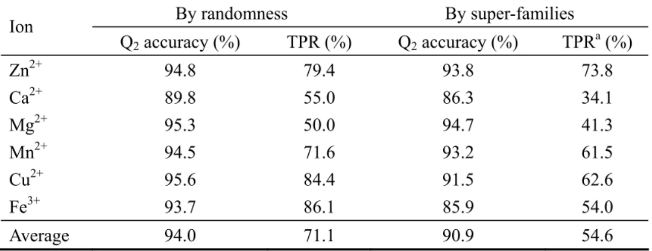
(13) TPR =. TP TP + FN ,. (3). FPR =. FP FP + TN .. (4). and the FPR is given by. The calculation of TPR at 5% FPR is in the process of drawing the ROC23 curve. For each testing case, the SVM outputs the probabilities of the two class labels. Normally, the decision threshold is 0.5, so the class with higher probability is the predicted result of the SVM. Alternatively, we can test various threshold values to verify the sensitivity and specificity with respect to each threshold value. In this work, the threshold ranges from 0.001 to 0.999, increasing by 0.001 each time. If the probability of a testing case is larger than the threshold, it is considered as “positive”; otherwise, it is considered as “negative”. Therefore each threshold value will produce a group of TPR and FPR, which decides a point on the ROC curve. Given an FPR value, we can get the respective TPR value.. 3 RESULTS 3.1 Datasets The data originally retrieved from PDB include more than seven thousand structures with more than twenty thousand chains at the time of Nov 2004. After the pre-processing described in the method section, we got 1063 chains distributed in 361 SCOP super-families. These numbers do not agree with the sum of those from the six metal ions owing to some chains may bind more than one kind of ions. The datasets are listed in Table 1. The all protein chains used in this study are listed in Appendix. 3.2 The prediction performance The overall prediction accuracy Q2 achieves 97.4% and TPR is 46.2% at 5% FPR. In this experiment, the non-site region is defined as the region outside the 21Å radius from each metal ion in the chain. The chains are grouped according to SCOP super-families such that the. 7.

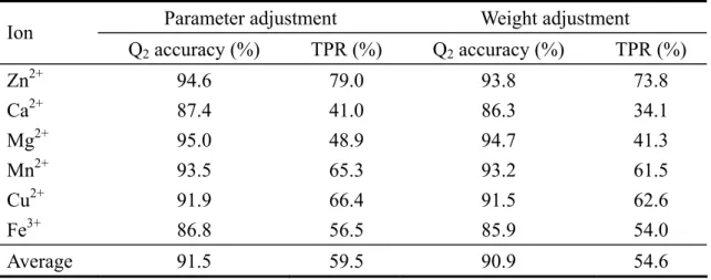
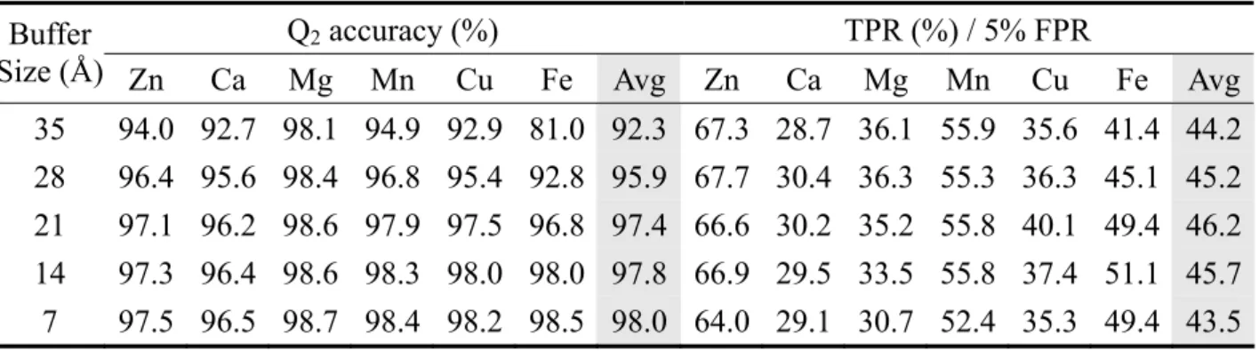
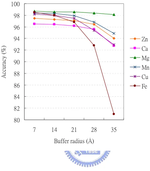
(14) chains in the testing sets will not be in the same super-family as those in the training sets. Therefore the chains belong to the same super-family will be grouped together in the training or testing sets. All the super-families are randomly divided into five groups for fivefold cross-validation. 3.3 Comparison between different grouping methods Besides the grouping with respect to super-families, we also do the grouping that randomly divides all the chains. The cross-validation results, as expected, are somewhat better than that of grouping by super-families due to some homologs in the testing sets have been trained before the prediction. The comparison of the two grouping methods is listed in Table 2. 3.4 The two SVM training strategy Despite the good prediction performance of SVM, it spends much time on parameters selection. Instead of adjusting parameter, we can adjust the weights of the two classes. The weight adjustment is based on the sizes of the two sets; we use the size of the smaller set as the weight for the larger set and vice versa. In contrast to parameter adjustment that the number of times of the training processes depend on how many groups of parameters tried, the training process for weight adjustment executes just once. The results are just a little worse than the best ones done by parameter adjustment. All other calculations are done by adjusting weights of the two classes. The results are listed in Table 3. 3.5 Effect of different radii for defining a non-site residue By using 7Å as the radius to define non-site residues, all residues in the sequence except site residues are regarded as non-site residues. As a result, the amount of the generated input data is large and may contain some ambiguous data coming from residues near the site region. A buffer zone is defined to be a shell enclosed by two concentric circles centered at the metal ion. The radius of the inner circle is 7Å, and several different radii are tried for the outer circle. The models are produced for each radius. The performance of different training models is evaluated by its accuracy to predict the 7Å testing set. Figure 13 and 14 show the accuracy. 8.

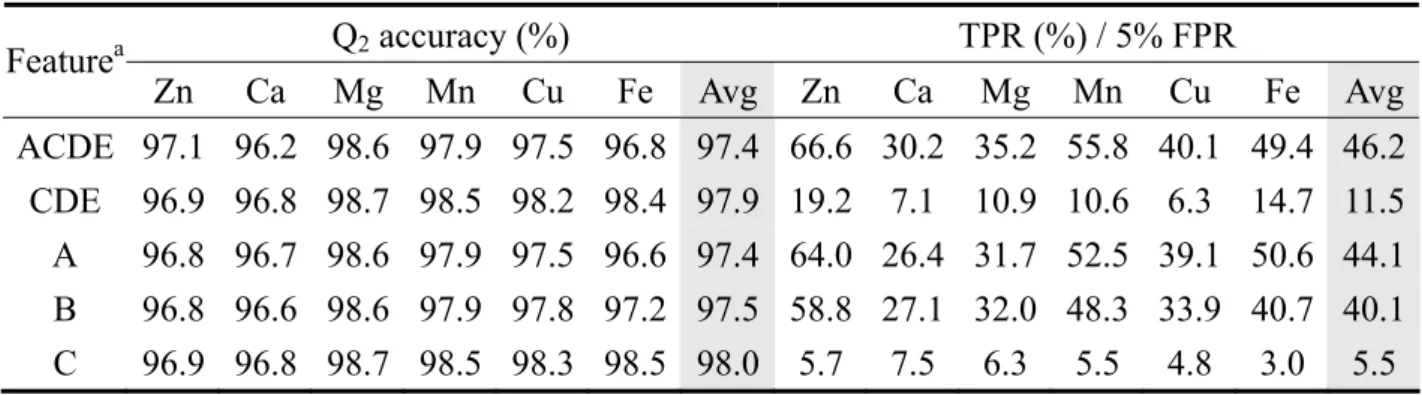
(15) and the true positive rate versus different models. Figure 15 shows the ROC curves of different classifiers for each metal ion. Table 4 lists the complete results for different models. 3.6 Comparison among different coding features The features used to encode the residues include PSSM, secondary structures, solvent accessibility, and distance matrix. The best results are given by combining all these features into one feature vector. Different features have different discriminating abilities. We separate the features and compare the prediction performance of each feature. We also compare the results with those from sequence PSSM, which is generated from residues local in primary sequence. The results are listed in Table 5. The ROC curves of each feature for six metal ions are showed as Figure 16 to Figure 21. 3.7 Comparison with previous work We use the same coding scheme as Sodhi’s, but we choose different radii for defining non-site residues. Instead of using artificial neural network for training and testing, we use SVM to perform the classification tasks. Our results from the 21Å training model achieves a 97.4% overall prediction accuracy compared to 94.5% and 46.2% TPR at 5% FPR compared to 39.2%. The comparison is listed in Table 6.. 4 DISCUSSIONS In identifying functional relevance residues in proteins, previous studies11,21,24 have shown that the machine learning approach is an effective way to discriminate the site residues from non-site residues. The SVM method is used in this study to predict the metal-binding site residues and gives consistent results. By comparing the performance of each coding feature, it is obvious that the ability to identify the site residues with a high accuracy comes from the sequence information as well as the structure information. The combination of structural and sequence information improves the quality of prediction11,24. Using SVM, this work is comparable with the recent work using artificial neural network11.. 9.

(16) When doing n-fold cross validation, the dataset is divided into n subsets, and the evaluation process repeats n times. Each time, one of the n subsets is taken as the test set, and the other n-1 subsets are taken as one training set as a whole. The division of the dataset is usually by random18,19. In this study we divide the dataset according to the super-family of each instance in the dataset. The reason for using this approach is that we can detect the site in proteins as if they are in new super-families since the training and testing set do not have proteins in common super-families11. We compared these two approaches for dividing the dataset. The one with random division has the better results because of the knowledge of the homologs. In practice, since we already have a library for all proteins with known structures, the homology information can be utilized to improve the prediction accuracy; if it fails to have the homologs, it is just the case to predict the proteins in new super-families. Therefore the performance resulting from grouping by super-families can be regarded as the worst case situation. The site or non-site residues are defined as within or without a certain distance to the metal ion. The value of this distance has a direct impact on the amount of site or non-site residues. The site residues in this study are defined to be within the sphere of radius 7Å centered at the metal ion. We try several different cut-off values to define the non-site residues and find that not only the training time but also the TPR improves as the radius increases. By using a small radius, more residues close to the binding site (but still outside the 7Å radius) are taken as non-site residues. These residues resemble the real site residues in position and nature. This may cause the SVM difficult to distinguish the site residues from non-site residues. Choosing the limited number of non-site residues as the control group10 may prevent the classifier from over-fitting and improve the sensitivity to detect site residues. The results showed in Table 5 confirmed this point. The best prediction results do not occur at the training model produced by 7Å cut-off value for non-site residues nor at that by 35Å. The 35Å radius is so large an area such that few non-site residues can be included in the training set, resulting in the scarcity of training data.. 10.

(17) From the results we notice that the prediction accuracy and TPR of calcium ion is much lower compared to other metal ions. This trend is consistent with the results by Sodhi, et al. (2004). The ionic radius of calcium is 0.95Å, 0.46Å for manganese, 0.645Å for iron, 0.65Å for magnesium, 0.73Å for copper, and 0.75Å for zinc25-27. As a result, the ion-oxygen bond length is longer for calcium ion than the other ions listed here28. They also show that calcium ions have a strong binding affinity to oxygen atoms, resulting in the constrained choice of ligands. Due to the same decision radius of 7Å for all metal ions, the longer ion-oxygen bond length of calcium ion may prevent the ligands from been included in the site residues. This situation may lead to the lower prediction accuracy and also the longer training time. As a conclusion, it has been shown that the coding scheme that combines sequence profile and structural features is capable of represent the characteristics of particular site patterns. Protein structures can be viewed as residue interaction graphs (RIGs)29, a simplified model to represent the complex protein 3D structures. This model is used to identify active sites, ligand-binding and evolutionary conserved residues. Bagley and Altman (1995) use a fixed number of concentric shells to collect the features stored in the vicinity of the calcium ion. This raises a possibility to encode the spatial distribution of properties of residues in the shells centered at particular residue. This new direction may lead to more efficient calculations and more accurate predictions.. 11.

(18) REFERENCES 1. 2. 3. 4. 5. 6. 7. 8. 9. 10. 11.. 12. 13. 14.. 15. 16. 17.. 18.. Ibers JA, Holm RH. Modeling coordination sites in metallobiomolecules. Science 1980;209(4453):223-235. Babor M, Greenblatt HM, Edelman M, Sobolev V. Flexibility of metal binding sites in proteins on a database scale. Proteins 2005;59(2):221-230. Lu Y, Berry SM, Pfister TD. Engineering novel metalloproteins: design of metal-binding sites into native protein scaffolds. Chem Rev 2001;101(10):3047-3080. Thompson KH, Orvig C. Boon and bane of metal ions in medicine. Science 2003;300(5621):936-939. Dobson PD, Doig AJ. Distinguishing enzyme structures from non-enzymes without alignments. J Mol Biol 2003;330(4):771-783. Chothia C. Proteins. One thousand families for the molecular biologist. Nature 1992;357(6379):543-544. Dobson PD, Doig AJ. Predicting enzyme class from protein structure without alignments. J Mol Biol 2005;345(1):187-199. Charniak E. Bayesian networks without tears. AI Magazine 1991;12(4):50-63. Vapnik V. The Nature of Statistical Learning Theory. New York: Springer-Verlag; 1995. Bagley SC, Altman RB. Characterizing the microenvironment surrounding protein sites. Protein Sci 1995;4(4):622-635. Sodhi JS, Bryson K, McGuffin LJ, Ward JJ, Wernisch L, Jones DT. Predicting metal-binding site residues in low-resolution structural models. J Mol Biol 2004;342(1):307-320. Berman HM, Westbrook J, Feng Z, Gilliland G, Bhat TN, Weissig H, Shindyalov IN, Bourne PE. The Protein Data Bank. Nucleic Acids Res 2000;28(1):235-242. Zhang C, Kim SH. Environment-dependent residue contact energies for proteins. Proc Natl Acad Sci U S A 2000;97(6):2550-2555. Murzin AG, Brenner SE, Hubbard T, Chothia C. SCOP: a structural classification of proteins database for the investigation of sequences and structures. J Mol Biol 1995;247(4):536-540. Altschul SF, Gish W, Miller W, Myers EW, Lipman DJ. Basic local alignment search tool. J Mol Biol 1990;215(3):403-410. Kabsch W, Sander C. Dictionary of protein secondary structure: pattern recognition of hydrogen-bonded and geometrical features. Biopolymers 1983;22(12):2577-2637. Altschul SF, Madden TL, Schaffer AA, Zhang J, Zhang Z, Miller W, Lipman DJ. Gapped BLAST and PSI-BLAST: a new generation of protein database search programs. Nucleic Acids Res 1997;25(17):3389-3402. Hua S, Sun Z. A novel method of protein secondary structure prediction with high. 12.

(19) 19.. 20.. 21. 22. 23. 24. 25. 26. 27. 28. 29.. segment overlap measure: support vector machine approach. J Mol Biol 2001;308(2):397-407. Yu CS, Wang JY, Yang JM, Lyu PC, Lin CJ, Hwang JK. Fine-grained protein fold assignment by support vector machines using generalized npeptide coding schemes and jury voting from multiple-parameter sets. Proteins 2003;50(4):531-536. Chen YC, Lin YS, Lin CJ, Hwang JK. Prediction of the bonding states of cysteines using the support vector machines based on multiple feature vectors and cysteine state sequences. Proteins 2004;55(4):1036-1042. Yan C, Dobbs D, Honavar V. A two-stage classifier for identification of protein-protein interface residues. Bioinformatics 2004;20 Suppl 1:I371-I378. Chang C-C, Lin C-J. LIBSVM: a library for support vector machines. Software available from http://www.csie.ntu.edu.tw/~cjlin/libsvm. 2001. Metz CE. Basic principles of ROC analysis. Semin Nucl Med 1978;8(4):283-298. Gutteridge A, Bartlett GJ, Thornton JM. Using a neural network and spatial clustering to predict the location of active sites in enzymes. J Mol Biol 2003;330(4):719-734. Pauling L. The nature of the chemical bond. Cornell University Press. Ithaca, NY. 1960. Brown ID. What factors determine cation coordination numbers? Acta Cryst 1988;B44:545-553. Barbalace K, Barbalace R, Barbalace J. Periodic Table of Elements Sorted by Ionic Radius. http://environmentalchemistrycom/ 1995. Katz AK, Glusker JP, Beebe SA, Bock CW. Calcium Ion Coordination: A Comparison with That of Beryllium, Magnesium, and Zinc. J Am Chem Soc 1996;118:5752-5763. Amitai G, Shemesh A, Sitbon E, Shklar M, Netanely D, Venger I, Pietrokovski S. Network analysis of protein structures identifies functional residues. J Mol Biol 2004;344(4):1135-1146.. 13.

(20) TABLES Table 1. The statistics of the datasets used in this work No. PDB No. SCOP No. metal Ion chainsa super-families ions 2+ Zn 372 202 613 2+ Ca 273 144 576 2+ Mg 261 129 357 2+ Mn 110 66 173 2+ Cu 47 28 74 3+ Fe 51 25 66 a. These data are collected at the time of Nov 2004.. 14.

(21) Table 2. Comparison of the two grouping methods: by randomness and by super-families Ion. By randomness. By super-families. Q2 accuracy (%). TPR (%). Q2 accuracy (%). TPRa (%). Zn2+ Ca2+ Mg2+ Mn2+ Cu2+ Fe3+. 94.8 89.8 95.3 94.5 95.6 93.7. 79.4 55.0 50.0 71.6 84.4 86.1. 93.8 86.3 94.7 93.2 91.5 85.9. 73.8 34.1 41.3 61.5 62.6 54.0. Average. 94.0. 71.1. 90.9. 54.6. The cutoff radius for non-site residues is 35Å. a This is the true positive rate (TPR) at 5% false positive rate (FPR).. 15.

(22) Table 3. Comparison of the two training options of SVM: weight and parameter adjustment Ion. Parameter adjustment. Weight adjustment. Q2 accuracy (%). TPR (%). Q2 accuracy (%). TPR (%). 2+. Zn Ca2+ Mg2+ Mn2+ Cu2+ Fe3+. 94.6 87.4 95.0 93.5 91.9 86.8. 79.0 41.0 48.9 65.3 66.4 56.5. 93.8 86.3 94.7 93.2 91.5 85.9. 73.8 34.1 41.3 61.5 62.6 54.0. Average. 91.5. 59.5. 90.9. 54.6. The cutoff radius for non-site residues is 35Å.. 16.

(23) Table 4. Comparison among different buffer sizes Buffer Size (Å) Zn 35 28 21 14 7. 94.0 96.4 97.1 97.3 97.5. Q2 accuracy (%). TPR (%) / 5% FPR. Ca. Mg. Mn. Cu. Fe. Avg. Zn. Ca. Mg. Mn. Cu. Fe. Avg. 92.7 95.6 96.2 96.4 96.5. 98.1 98.4 98.6 98.6 98.7. 94.9 96.8 97.9 98.3 98.4. 92.9 95.4 97.5 98.0 98.2. 81.0 92.8 96.8 98.0 98.5. 92.3 95.9 97.4 97.8 98.0. 67.3 67.7 66.6 66.9 64.0. 28.7 30.4 30.2 29.5 29.1. 36.1 36.3 35.2 33.5 30.7. 55.9 55.3 55.8 55.8 52.4. 35.6 36.3 40.1 37.4 35.3. 41.4 45.1 49.4 51.1 49.4. 44.2 45.2 46.2 45.7 43.5. The testing set is of 7Å buffer size. The training sets are of different buffer sizes ranging from 7Å to 35Å.. 17.

(24) Table 5. Comparison among different coding features Featurea ACDE CDE A B C. Q2 accuracy (%). TPR (%) / 5% FPR. Zn. Ca. Mg. Mn. Cu. Fe. Avg. 97.1 96.9 96.8 96.8 96.9. 96.2 96.8 96.7 96.6 96.8. 98.6 98.7 98.6 98.6 98.7. 97.9 98.5 97.9 97.9 98.5. 97.5 98.2 97.5 97.8 98.3. 96.8 98.4 96.6 97.2 98.5. 97.4 97.9 97.4 97.5 98.0. a. Zn. Ca. Mg. Mn. Cu. 66.6 30.2 35.2 55.8 40.1 19.2 7.1 10.9 10.6 6.3 64.0 26.4 31.7 52.5 39.1 58.8 27.1 32.0 48.3 33.9 5.7 7.5 6.3 5.5 4.8. Fe. Avg. 49.4 14.7 50.6 40.7 3.0. 46.2 11.5 44.1 40.1 5.5. A: Site PSSM, B: Sequence PSSM, C: Secondary Structure, D: Solvent Accessibility, E: Distance Matrix. 18.

(25) Table 6. Comparison with Sodhi’s results Ion. JJLina. Sodhi Q2 accuracy (%). TPR (%). Q2 accuracy (%). TPR (%). 2+. Zn Ca2+ Mg2+ Mn2+ Cu2+ Fe3+. 94.6 93.9 94.2 94.7 94.9 94.9. 47.8 30.4 32.4 38.8 36.2 48.8. 97.1 96.2 98.6 97.9 97.5 96.8. 66.6 30.2 35.2 55.8 40.1 49.4. Average. 94.5. 39.1. 97.4. 46.2. a. The cutoff radius for non-site residues is 21Å.. 19.

(26) FIGURE CAPTIONS Figure 1. PDBid 1A8A, with coordination number 4. The sphere in magenta is the calcium ion, and the sphere in red is the oxygen atom. The smaller figure at upper-left corner is the full-view of the protein, and the larger figure is the magnified view of one of the metal-binding site. Figure 2. PDBid 1G4Y, with coordination number 5. Figure 3. PDBid 1I76, with coordination number 6. Figure 4. PDBid 1GCI, with coordination number 7. Figure 5. PDBid 1ARU, with coordination number 8. Figure 6. The data pre-processing procedure. We obtain the original sequences from PDB. The chain that is DNA or RNA is filtered out. The length of the chain must be at least 50 residues. The chain must contain at least one metal ion. The information of SCOP super-families, DSSP secondary structure, and solvent accessibility is retrieved and processed. The DSSP sequence is used to generate the PSSM of the sequence. Finally the dataset contains 1063 protein chains. Figure 7. Definition of the site residues. Residues are the site residues if their main chain atoms (N, Cα, C) lie within the 7Å radius sphere centered at the metal ion. The figure shows the Benzoylformate Decarboxylase structure with PDBid 1BFD. Figure 8. Definition of buffer zone and the non-site residues. The buffer zone is located between the inner and outer sphere. The radius of the inner sphere is 7Å, and the radius of the outer sphere ranges from 7Å to 35Å. The non-site region is located outside the outer sphere. Residues located at the non-site region are the non-site residues. The figure shows the Benzoylformate Decarboxylase structure with PDBid 1BFD. Figure 9. Coding information of PSSM. The 20 scores of the next residue are appended to the rear of the scores of the present residue. Figure 10. Coding information of DSSP. The 40 scores of the DSSP are appended to the rear. 20.

(27) of the PSSM scores. Figure 11. Coding information of distance matrix of Cβ atoms of residue neighbors. The 45 distances are appended to the rear of the DSSP scores. Figure 12. System flowchart Figure 13. Comparison of the accuracy among different buffer sizes. The 7Å testing set is predicted by all the training models of different radii. Figure 14. Comparison of the true positive rate (TPR) among different buffer sizes. Figure 15. ROC curves of different classifiers. The results are from buffer size of 21Å. Figure 16. ROC curves of each feature. A: Site PSSM, B: Sequence PSSM, C: Secondary structure, D: Solvent accessibility, E: Distance matrix. (a) Fe3+ ion. (b) Cu2+ ion. (c) Mn2+ ion. (d) Mg2+ ion. (e) Ca2+ ion. (f) Zn2+ ion.. 21.

(28) FIGURES Figure 1. 22.

(29) Figure 2. 23.

(30) Figure 3. 24.

(31) Figure 4. 25.

(32) Figure 5. 26.

(33) Figure 6. Original sequence. Filter out the chain that is DNA or RNA. Filter out the chain with sequence length less than 50. Filter out the chain without metal ion. Identifying SCOP classification at the superfamily level. Identifying DSSP secondary structure and solvent accessibility. The dataset. 27.

(34) Figure 7. Binding site residue. Non-binding site residue. 28.

(35) Figure 8. Buffer Zone Binding site residue. Non-binding site residue. 29.

(36) Figure 9 PSSM … … 13 14 15 16 17 18 19 20 21 22 23 24 25 26 27 28 29 … …. … … K E A F S L F D K D G D G T I T T … …. 20 23 19 25 27 17 16 21 31 26. D G F G I S F K E T. … … 16 F 17 S 18 L 19 F 20 D 21 K 22 D 23 G 24 D 25 G 26 T 27 I 28 T 29 T 30 K 31 E … …. 1 2 …… 20 -4 -5 …… -3 1. -5 -1 -1 -5 -4 -1 -4 -2 -3 -3 0 -4 0 1 -1 -3. -6 2 -1 -6 -5 3 -1 1 -2 -4 1 -6 -3 -2 -1 -3. -6 2 0 -6 -2 -2 4 3 2 -1 -2 -6 0 -2 1 -2. -7 3 -4 -7 8 -2 6 -2 6 -3 -2 -6 3 -5 2 3. -5 0 -4 -5 -6 -5 -6 -2 -3 -4 3 -4 -4 1 -6 -6. -6 1 -3 -6 -3 1 0 0 -2 -3 0 -6 -2 -2 0 3. -6 1 -1 -6 -1 -2 1 -2 1 -3 -2 -6 -1 -3 3 6. -5 -2 -4 -6 -4 -3 -3 5 -2 7 -5 -7 -2 -4 -1 -5. -4 -3 -5 -3 -2 -1 -2 -2 -4 -5 0 -6 -1 -2 2 -2. 1 2 …… 20 …… ……. -3 -4 0 1 -4 -2 -5 -6 -5 -6 -3 8 -5 -1 -5 -6. -2 -2 4 0 -6 -5 -5 -6 -6 -6 -3 0 -3 -1 -3 -5. 1. -6 2 -3 -6 -4 5 -1 3 0 -3 3 -6 -1 0 4 -1. -3 -2 5 3 -6 0 -5 -5 -5 -1 -3 0 -2 -3 -4 0. 9 -5 -2 8 -6 -5 -6 -6 -6 -3 2 -3 -5 2 -6 -5. -7 -4 -5 -6 -4 -3 -5 -4 -4 -5 -5 -6 -1 0 -4 -4. -5 2 -1 -5 -3 -1 -3 -2 3 -2 1 -5 3 -1 0 -2. 2 …… 20. -2 1 …… -6 …… …… -3 -3 …… -4 2 10. Total: 10 * 20 = 200 (PSSM scores). 30. -5 -1 -3 -4 -4 3 0 -4 0 -4 3 -4 5 3 -1 -2. -2 -6 -5 -2 -7 -6 -7 -6 -7 -5 -1 -6 -6 -4 -6 -6. 1 -5 -3 2 -6 -3 -5 -5 -5 -6 2 -4 -4 4 -3 -5. -4 -4 -1 -2 -3 -3 -2 -6 -5 -6 -2 2 -4 1 -5 -4.

(37) Figure 10 DSSP Secondary structure … … 13 14 15 16 17 18 19 20 21 22 23 24 25 26 27 28 29 … …. … … K E A F S L F D K D G D G T I T T … …. 0 0 1 1. 20 23 19 25 27 17 16 21 31 26. D G F G I S F K E T. 0 0 1 2. … … 16 F 17 S 18 L 19 F 20 D 21 K 22 D 23 G 24 D 25 G 26 T 27 I 28 T 29 T 30 K 31 E … …. H H H H. >X 3< << << >< T 3 T 3 < S S E E > H > H > H >. S+ S+ S+ S+ + S+ S+ SS+ -A -A S+ S+ S+. …… 0 1 0 10. Solvent accessibility 0 0 0 0 0 0 0 0 0 0 61 60 0 0 0 0. 0 0 0 0 0 0 0 0 0 0 0A 0A 0 0 0 0. 14 1. 12 73 100 45 14 113 110 56 95 32 30 7 28 7 116 17. 56 2. …… 30 10. Total: 10 * 3 + 10 * 1 = 40 (DSSP scores). 31.

(38) Figure 11 Distance matrix of Cβ atoms 20 23 19 25 27 17 16 21 31 26. D G F G I S F K E T. 23 G 4.692. 19 F 5.131 9.599. 25 G 5.397 5.532 9.824. 27 I 5.416 9.512 4.559 7.815. 17 S 5.691 7.258 7.418 9.153 10.125. 16 F 21 K 31 E 26 T 5.743 6.288 6.403 6.806 9.342 7.031 9.127 8.386 6.090 7.315 5.662 9.515 7.907 10.673 10.212 4.656 7.459 8.684 5.156 5.665 5.333 9.062 10.924 12.066 11.222 10.690 9.782 4.848 10.825 8.423. Total: 10 * 9 / 2 = 45 (distances). 32.

(39) Figure 12. PDB. Data pre-processing. 25% sequence identity clustering. Dataset PSSM. DSSP (SS, ACC). Encoding. Distance Matrix. SVM input file. SVM training. Fivefold cross-validation. Performance Evaluation. 33.

(40) Figure 13. 100 98. Accuracy (%). 96 94. Zn. 92. Ca Mg. 90. Mn. 88. Cu. 86. Fe. 84 82 80 7. 14. 21. 28. Buffer radius (Å). 34. 35.

(41) Figure 14. 70 65. TPR (%). 60 55. Zn. 50. Ca Mg. 45. Mn. 40. Cu. 35. Fe. 30 25 20 7. 14. 21. 28. Buffer radius (Å). 35. 35.

(42) Figure 15 1 0.9 0.8 0.7 Fe Cu Mn Mg Ca Zn. TPR (%). 0.6 0.5 0.4 0.3 0.2 0.1 0 0. 0.05. 0.1. 0.15. 0.2. 0.25 FPR (%). 36. 0.3. 0.35. 0.4. 0.45. 0.5.

(43) Figure 16 Fe 1 0.9 0.8 0.7 A B C C+D+E A+C+D+E. TPR (%). 0.6 0.5 0.4 0.3 0.2 0.1 0 0. 0.02. 0.04. 0.06. 0.08. 0.1 FPR (%). 37. 0.12. 0.14. 0.16. 0.18. 0.2.

(44) Figure 17 Cu 1 0.9 0.8 0.7 A B C C+D+E A+C+D+E. TPR (%). 0.6 0.5 0.4 0.3 0.2 0.1 0 0. 0.02. 0.04. 0.06. 0.08. 0.1 FPR (%). 38. 0.12. 0.14. 0.16. 0.18. 0.2.

(45) Figure 18 Mn 1 0.9 0.8 0.7 A B C C+D+E A+C+D+E. TPR (%). 0.6 0.5 0.4 0.3 0.2 0.1 0 0. 0.02. 0.04. 0.06. 0.08. 0.1 FPR (%). 39. 0.12. 0.14. 0.16. 0.18. 0.2.

(46) Figure 19 Mg 1 0.9 0.8 0.7 A B C C+D+E A+C+D+E. TPR (%). 0.6 0.5 0.4 0.3 0.2 0.1 0 0. 0.02. 0.04. 0.06. 0.08. 0.1 FPR (%). 40. 0.12. 0.14. 0.16. 0.18. 0.2.

(47) Figure 20 Ca 1 0.9 0.8 0.7 A B C C+D+E A+C+D+E. TPR (%). 0.6 0.5 0.4 0.3 0.2 0.1 0 0. 0.02. 0.04. 0.06. 0.08. 0.1 FPR (%). 41. 0.12. 0.14. 0.16. 0.18. 0.2.

(48) Figure 21 Zn 1 0.9 0.8 0.7 A B C C+D+E A+C+D+E. TPR (%). 0.6 0.5 0.4 0.3 0.2 0.1 0 0. 0.02. 0.04. 0.06. 0.08. 0.1 FPR (%). 42. 0.12. 0.14. 0.16. 0.18. 0.2.

(49) APPENDIX Appendix 1. Protein chains containing Fe3+ ions Fe 1EO2:B 1GUP:A 1NX4:B 1BK0:_ 1LTV:A 1GVG:A. 1COJ:A 1QGH:A 1NMO:A 1RCW:B 1RXG:_ 1XSM:_. 1NF6:F 2PAH:A 1B71:A 1GV8:A 2AHJ:C 1J2C:A. 1SUV:E 1DO6:A 1O9R:A 1K6W:A 1J3Q:A 1LM6:A. 1B13:A 1NDO:A 1HU9:A 1PHZ:A 1LM4:A 1FHA:_. 43. 1RSV:B 1OQU:C 1D9Y:A 1M63:A 1DYT:A 1DFX:_. 1B0L:A 1DLM:A 1UN7:A 1O2D:B 1FRF:L. 1OHV:A 1OQ4:A 1Q0C:A 1QHW:A 1GP5:A. 1KBP:A 1MMO:D 1EIQ:A 1GY9:A 1LNB:E.

(50) Appendix 2. Protein chains containing Cu2+ ions Cu 1EQW:B 1ID2:A 1ODB:A 1LCF:_ 7ICJ:A 1OQ6:A. 1CC3:A 1M56:B 1OV8:A 1GOF:_ 1ARM:_ 1FVS:A. 1ET7:A 1IBY:A 1N9E:A 1GW0:A 1KYR:A. 1BAW:A 1A2V:A 1NOL:_ 2OXI:A 1AND:_. 1OAC:B 1AOZ:A 1FSR:A 1BUG:A 1IAA:_. 44. 1M56:A 1HCY:_ 1GMW:A 1A8V:B 1QD0:A. 1H1I:B 1A65:A 1N68:A 1JER:_ 1AQP:_. 1AV4:_ 1GY2:A 1LNL:A 1KCW:_ 1OT4:A. 1BQK:_ 1THO:_ 1OPM:A 1GSK:A 1UKU:A.

(51) Appendix 3. Protein chains containing Mn2+ ions Mn 1BJQ:B 1BFR:A 1N51:A 1FJM:A 1IMC:B 1GQ6:B 1GX6:A 1CNZ:A 1OF2:A 1VJ2:A 1MNP:_ 1ZIP:_ 2PAL:_. 1AZD:A 1GQ2:A 1CHR:A 1N1H:A 1G0I:A 1NOM:_ 1FA0:B 1CDK:A 1UT5:B 1NR0:A 1FOA:A 1FI2:A 1IGV:A. 1HQF:A 1ZQL:A 1O0R:B 1ITW:A 1RF7:_ 1G5B:B 1N1P:A 1II7:A 1QH3:A 1EF2:A 1LNC:E 1INO:_. 1KFL:A 1G8O:A 1K20:A 1QMG:A 1GX1:A 1I50:A 1KHW:B 1I0B:A 1KWS:A 1HK8:A 1A76:_ 1JAI:_. 1GV3:A 1FSA:A 1MHP:B 1O98:A 1C39:A 1L5G:A 1ECC:A 1KGZ:B 1M4Z:B 1AQ2:_ 1RZD:_ 1NCY:_. 45. 1F3W:A 1M6V:A 1NHX:A 1A0D:A 1JFZ:B 1JQN:A 1MM8:A 1IPS:A 1MQW:A 1F5A:A 1LL2:A 1NZ5:A. 1F1H:A 1E6A:A 1HO5:A 1DE6:A 1ON2:A 1KSI:A 1ELS:_ 1O6K:A 1J53:A 3UAG:A 1H7Q:A 1G15:A. 1DID:A 1HX3:B 1J2T:A 1JPR:B 1M0D:A 1LV5:A 1LWD:A 1CPO:_ 1GN8:A 1IR6:A 1K23:D 1JLK:A. 1HHS:A 1FQW:A 1FUI:A 1KGP:A 1UW8:A 1L5G:B 1OLX:A 1IG1:A 1A5V:_ 1A6Q:_ 1DAH:_ 1J25:A.

(52) Appendix 4. Protein chains containing Mg2+ ions Mg 1BGL:A 1A49:A 1EC9:D 1FRF:L 1P8F:A 1QMZ:A 1II0:B 1HBN:A 1K3C:A 1H7U:A 1QL0:A 1ITZ:A 1PFK:A 1HQM:D 3PMG:A 1JBV:A 1GOL:_ 1MC3:A 1H7Q:A 1KQM:B 1N52:A 1O6T:A 1OLU:A 1L8Q:A 1H74:B 1HW6:A 1IRU:I 1H6P:A 1VSD:_. 1AN0:A 1EBG:A 1M34:E 1AF6:A 1MXA:_ 1J7L:A 1MX0:C 1BWF:O 1YVE:I 1RK2:B 1IW7:A 1EQR:A 1IOV:_ 1IW7:C 1UN9:A 1OD5:A 1IXY:B 1MUM:A 1GKB:A 1L0O:A 1GM5:A 1MXG:A 1BG0:_ 1FHV:A 1CSN:_ 1EYE:A 1IRU:1 1ETU:_ 1GMI:A. 1DIE:A 1OHH:D 1BYU:B 1G69:B 1G3U:A 1HBM:C 1MIV:A 1AUK:_ 1NJ1:A 1M1B:A 1NR9:A 1H7A:A 1FYD:A 1GL9:B 1AMU:A 1FNN:A 1IW7:F 2PRN:_ 1A82:_ 1KTG:A 1FNM:A 2UAG:A 1QLG:A 1ODS:A 1TFR:_ 1LDF:A 1OPR:_ 1IWL:A 1F7R:A. 1BWV:A 1EYI:A 1CG0:A 1OFH:G 1JGT:B 1F5S:A 1NMP:A 1GKI:B 1HBN:B 1E0J:B 1BJY:B 1GPM:C 1H65:A 1G8X:A 1SH3:B 1J58:A 1NE9:A 1VFN:_ 1LVH:A 1CMC:A 1F5N:A 1AQF:E 1EZW:A 1A77:_ 1I44:A 1NXQ:A 1N0W:A 1NQZ:A 1CS3:A. 1N0H:A 1AGR:A 1ATR:_ 1EFT:_ 1ECB:C 1PT6:B 2AKY:_ 1DTN:_ 1KCZ:A 1OES:A 1OE0:A 1EHI:A 1H1D:A 1L8A:A 1M0W:A 1J1C:B 8ICI:A 1F1Z:A 1N9K:A 1NLQ:A 1NQE:A 1QS0:A 1L3R:E 1GSA:_ 1JWY:B 1HK7:A 1OUO:A 1QF8:A 1HXI:A. 46. 1BR1:A 1HUR:A 1ZPD:A 1F4V:A 13PK:A 1NFS:B 1QEZ:A 1GQC:A 1EYZ:A 1GS5:A 1KO5:A 1K9Y:A 1L4Y:A 1FW6:A 1GQY:B 1OC7:A 1GKZ:A 1G6H:A 1UUT:A 1UN6:C 1H1L:B 1INP:_ 1GS6:X 1JP4:A 1IAH:B 1NSF:_ 1IRU:X 1NZI:A 1HZ1:A. 1MAB:A 1N1Z:A 1F0J:A 1OCC:A 1GOJ:A 1HI0:P 1DY3:A 1N8W:A 1BXZ:A 1FEZ:A 1GRV:B 1UBW:_ 1HTW:A 1H16:A 1EWK:B 1N6M:A 1E19:A 1J9J:A 1IPP:A 1I3Q:A 1KA2:A 1HMV:B 1H3J:A 1NQ6:A 1JHZ:A 1DQN:A 1KHZ:B 1KWO:C 1IW7:O. 1EW2:A 1IV2:A 1CJB:C 1F8I:A 1GZG:A 1AON:A 1F7D:A 1OHF:C 1UR2:A 1DXE:A 1B8C:A 1GXB:D 1Q9S:A 1GQI:A 1BIF:_ 1NI4:A 1OBG:A 1IRU:G 1H56:A 1KC7:A 1BPM:_ 1IIR:A 1B62:A 1J1U:A 1K77:A 1QR0:A 1MH9:A 1R67:A 1IG5:A. 1MFR:A 1NUE:A 1E2F:A 1M3U:A 1JQV:A 1B0P:A 1IQ8:A 1N5Y:A 1ESN:A 1DEK:A 1GUS:A 1JX4:A 1IW7:D 1NUG:B 1HYO:B 1JMS:A 1H3I:A 1NUI:A 1L5Y:B 1D5A:A 1H1L:A 1E4G:T 1LP4:A 1IZC:A 1O6Y:A 1KYR:A 1NRJ:B 1ID0:A 1MOG:A.

(53) Appendix 5. Protein chains containing Ca2+ ions Ca 1BJQ:B 1CDG:_ 1BU4:_ 1AY0:A 1PK8:A 1E3X:A 1UYY:A 1B0P:A 1CB8:A 1F2O:A 1MPX:A 1LWH:A 1BMO:A 1DE4:C 1I82:A 1H0H:A 1N7U:A 1DCT:A 1RTG:_ 1GN1:F 1HDF:A 1NOL:_ 1CVR:A 1OKG:A 1RDR:_ 1B2L:A 2SAS:_ 1B1C:A 1TN3:_ 1F7L:A 1N7S:C. 1CVW:H 1EA7:A 1EGI:B 1AKL:_ 1ALV:A 1JDA:_ 1TNQ:_ 1F9D:A 1LPM:_ 1FF5:A 1B4N:A 1HYO:B 1QU0:C 1GXD:A 1J83:A 1J0M:A 1HDH:A 1IME:A 4SBV:A 1NL2:A 1K9U:A 1C8D:A 1LWS:A 1KA1:A 1E1A:A 1O7L:D 1M1U:A 1LF0:A 1POC:_ 2MCM:_ 1GUA:B. 1BM6:_ 1HTN:_ 1PVA:A 1GA1:A 1UMN:G 1A0S:P 1HP0:B 1HM8:A 1EAK:A 1BYH:_ 1UP8:A 1JI3:A 1OH4:A 1G21:B 1AG9:A 1KB0:A 1N2L:A 1UOC:A 1H1A:A 1EXZ:A 1GUN:A 1CLC:_ 1BAG:_ 1JX6:A 1GQ3:C 1ZQV:_ 2STV:_ 1K12:A 1J24:A 1IU9:A 1OHZ:B. 1AZD:A 1B2Y:A 1DR1:_ 2MSB:B 1C0F:S 1J6Z:A 2MAS:A 1C9U:B 1GTT:A 1I9B:A 1M56:A 1MNZ:A 1BYF:A 1J1N:A 2FHA:_ 1M9I:A 1MIO:B 1H6G:A 1I40:A 1C7K:A 1SU4:A 1JV2:B 1IKA:_ 1GXR:A 1BOB:_ 1J1T:A 1JE5:B 1ESL:_ 1GR3:A 1WAD:_. 1AYP:A 1QLS:A 1AXN:_ 1HQD:A 1LRW:A 1O88:A 1LNQ:A 1HPL:A 1CVM:A 1H6X:A 1E77:A 1H1V:G 1HT9:A 1N48:A 1UZJ:A 1CJY:A 1IA7:A 1L6R:A 1PRR:_ 1RLW:_ 1JV2:A 1BFD:_ 1H30:A 1E54:A 2POR:_ 1SLM:_ 1HQV:A 1GUI:A 1PK6:B 1SVY:_. 47. 1OMR:A 3LHM:_ 1MN1:_ 1Q5C:C 1FWX:A 1LVU:D 1FZD:A 2CEL:A 1EB7:A 1O8P:A 1R64:A 1ZQC:A 1F4N:A 1D0K:A 1DSY:A 1NBW:A 1DYK:A 1CPM:_ 1JTG:B 1IT4:A 1KIT:_ 1C7I:A 1JHN:A 1V04:A 1EZM:_ 1DAF:_ 1XYN:_ 1JB0:L 1AYO:B 1O6S:B. 1FJT:A 1N73:C 1OAC:B 1LW5:D 1DJW:B 1DTH:A 1HCU:B 1OLP:A 1GCA:_ 1L7L:A 2TAA:A 1KXR:B 1BG3:A 1TAD:C 2PSR:_ 1H3G:A 1OC6:A 1OUP:A 1E7D:A 1NQD:B 1BF2:_ 1FSU:_ 1QH4:D 2APR:_ 1NRW:A 4SBV:C 1NYA:A 1SRA:_ 5CHY:_ 2PLT:_. 1A4G:A 1B90:A 1STA:_ 1IZJ:A 1OAH:B 5STD:A 1E8U:B 1E5N:A 1E5J:A 1GZT:A 1O6V:A 2CBL:A 1UVN:A 1EGZ:A 1C07:A 1NQH:A 1G9U:A 1NNL:B 1NZI:B 1MJ2:B 1ACC:_ 1MU5:A 1NGI:_ 1OBR:_ 1URX:A 1PEX:_ 1B2V:A 1K5W:A 1J5U:A 1H4B:A. 1BGP:_ 1B09:A 1JKU:A 1M34:A 1L9M:B 1HL5:C 1LHN:A 1G0H:A 1G42:A 1FI5:A 1KTW:A 1FID:_ 1K1X:A 1NZY:A 1LMJ:A 1KFQ:A 1FMJ:A 1OTN:A 1NBC:A 1FZP:B 1N7D:A 5ENL:_ 1FBL:_ 1GXO:A 1JTD:A 1QV1:A 1V67:A 1VSI:_ 1DFX:_ 1HJ7:A.

(54) Appendix 6. Protein chains containing Zn2+ ions Zn 1E3E:A 1F57:A 1JD5:A 1TSR:A 1AKL:_ 1R3N:A 1CNQ:A 1I3Q:J 1B71:A 1DOS:A 1M2V:B 7MDH:B 1A74:A 1JTK:A 1JZQ:A 1C3R:A 1I6O:B 1GAX:A 1F83:A 1PV9:A 1UT8:B 1I9R:H 1QF8:A 1C7K:A 1D0Q:A 1UN6:C 1FAQ:_ 1CLC:_ 1PMI:_ 1NKX:A 1C8M:1 1AOL:_ 1FD9:A 1NKU:A 258L:A 1UV0:A 1RMD:_ 1G73:D 1F81:A 1G47:A 2ADR:_ 1JJD:A. 1EQW:B 1K1D:A 1GYT:A 1FBX:A 1KBP:A 1ZQT:A 1BH5:B 1SFO:B 1DY1:A 1AMP:_ 1HBM:D 1L9H:A 1F1M:A 1A2P:A 1M2O:A 1JR3:A 1LHN:A 1H3N:A 1KOL:A 1JR3:E 1MVH:A 1EU3:A 1BWN:A 2CUA:B 1NO5:B 1L0I:A 1MFT:A 1FSS:A 1CVR:A 1JK0:A 2EBN:_ 1A8L:_ 1JR9:A 1OEK:A 1FUK:A 1MZB:A 1UBD:C 1QBH:A 1CTL:_ 1RGO:A 1E53:A 1LPV:A. 1ZNC:A 1Q2R:A 1NVB:B 1IS8:A 1DE5:A 1IX1:A 1LR5:A 1JQG:A 1G5C:A 1F2O:A 2USH:B 1Q74:A 1E7D:A 1OI0:A 1EKM:A 1ET8:A 1EH6:A 1KFI:A 1XLL:A 1IBQ:A 1DK4:A 1L7O:B 1BT7:_ 1JOC:A 1MWQ:A 1I27:A 1PTQ:_ 1A8H:_ 1EUC:B 1H2M:A 1I6N:A 1SLM:_ 1AST:_ 1UVQ:B 1G73:B 1CPR:_ 1A6F:_ 1ZFP:E 1R79:A 1A7W:_ 1DL6:A 1F62:A. 1BM6:_ 1N4P:B 1H7R:A 1G2D:C 1GUP:A 1E4M:M 1HZ5:A 1UMY:D 1E67:A 1HI9:A 1KAH:B 1QH3:A 1GX1:A 1L3E:B 1GXD:A 1UDT:A 1BYF:A 1I7W:C 1JI3:A 1JAZ:A 1ML9:A 2AHJ:C 1VSH:_ 1M3V:A 1MR1:C 1TBN:_ 1TAQ:_ 1OAH:A 1HP7:A 1GR0:A 1GL4:A 1KYS:A 1GEN:_ 1IM5:A 1ODH:A 1Q9U:B 1AA0:_ 1JM7:B 1EXK:A 1CHC:_ 1UN6:D. 1EW2:A 1F0J:A 1Q3K:A 1DWV:A 1F30:A 1M2G:A 1I50:A 1ANV:_ 2HAP:C 1QRL:A 1EI6:A 1BKC:E 1IE0:A 1AJY:A 1GW6:A 1ALN:_ 1FWQ:A 1IRX:B 1P9W:A 1GUD:A 1NUI:A 1M55:A 1EB0:A 1DVF:D 2PSR:_ 2GAT:A 1OAO:C 1M7J:A 1FBL:_ 1D8D:A 1NZJ:A 1GPC:_ 1OCY:A 1JWQ:A 1VHH:_ 1LR0:A 1XPA:_ 1I3J:A 1E4U:A 1UW1:A 1BBO:_. 48. 1FJT:A 1A6Y:B 1H4S:A 1KZO:B 1ADD:_ 2NLL:B 1I3Q:C 1J8F:A 1PFV:A 1G12:A 1CG2:A 1AH7:_ 1RB7:A 4GAT:A 1H7A:A 1TON:_ 1BAW:A 1UQW:A 1M63:A 1NVT:A 1JW9:B 1LQW:A 1MBX:A 2A0B:_ 1OQJ:A 1HYI:A 1DMT:A 1LFW:A 1NL5:A 1OBR:_ 1AK0:_ 1DVP:A 4TSS:_ 1EB6:A 1R4V:A 1HML:_ 1M4M:A 1CY5:A 1IML:_ 1G25:A 1BOR:_. 1EZZ:B 1GT7:A 1HR6:D 1NLX:A 1HZY:A 1EPW:A 1ENR:_ 1IA9:B 1EAK:A 1F35:A 1LI7:A 1QR2:A 1JOE:A 1A7I:_ 4ENL:_ 1YEI:L 1JCC:C 1DDZ:A 1N25:A 1FXU:A 1L0Y:A 1TF6:D 2HRV:A 1I3O:E 1IQB:A 2DRP:D 1I1I:P 1QE3:A 1HKK:A 1CKO:_ 1VK6:A 1KEA:A 1B8T:A 1IWL:A 1F3Z:_ 1IJL:A 1JM7:A 1EYF:A 1BT0:A 1LV3:A 1EF4:A. 1LBC:B 1JDI:A 1KOG:A 1OCC:F 1DTH:A 1J36:A 1FSJ:B 1SML:A 1ODZ:A 3LVE:_ 1ITQ:A 1EKJ:G 1B6Z:A 1A1T:A 1MXD:A 1ZIN:_ 1HQM:D 1K2Y:X 1V33:A 1TOA:A 1M65:A 1L1O:C 1E31:B 1NN7:A 1LDJ:B 1MM2:A 1KWG:A 1LML:_ 1K9Z:A 1QHW:A 1CI3:M 1LBU:_ 1FIO:A 1OHT:A 4KMB:1 1E87:A 1M2A:A 1CIT:A 1MWZ:A 4MT2:_ 1IYM:A. 1A8T:A 1STE:_ 1NNJ:A 1CA1:_ 1PWU:A 1IQ8:A 1I3Q:I 1NJG:A 1FN9:A 1Q08:A 1JQ5:A 1K6Y:B 1ETE:A 1WJB:A 1UWY:A 1BI0:_ 1HWW:A 1IA7:A 1J79:A 1GVF:B 1H1Z:A 1H1O:A 1ODG:A 3CAO:A 1LLM:C 1YUI:A 1KLN:A 1DQ3:A 1ZAP:_ 1EZM:_ 1HW7:A 1PEG:B 1J3G:A 1DKH:A 1LBA:_ 1G3F:A 1XER:_ 1HFE:S 1DX8:A 1H7V:A 1IRN:_.

(55)