Low-Reynolds-number hydrodynamic interactions in a suspension of spherical particles with slip surfaces

(1)

Pergamon

P I I : S0009-2509(96)00514-3 o0o9 2509/97 $17.00 + 0.00

Low-Reynolds-number hydrodynamic

interactions in a suspension of spherical

particles with slip surfaces

**H u a n J. Keh* and Shih H. Chen t**

Department of Chemical Engineering, National Taiwan University, Taipei 106-17, Taiwan, Republic of China

(Received 11 March 1996)

Abstract--The motion of two rigid spherical particles in an arbitrary configuration in an infinite viscous fluid at low Reynolds numbers is considered. The fluid is allowed to slip at the surfaces of the spheres and the particles may differ in radius. The resistance and mobility functions that completely characterize the linear relations between the forces and torques and the translational and rotational velocities of the particles are analytically calculated in the quasi-steady limit using a method of twin multipole expansions. For each function, an expression of power series in r-1 is obtained, where r is the distance between the particle centers. The agreement between these expressions and the relevant results in the literature is quite good. Based on a microscopic model, the analytical results for two-sphere hydrodynamic interactions are used to find the effect of the volume fraction of particles of each type on the average settling velocities in a bounded suspension of slip spheres. Our results, presented in simple closed forms, agree very well with the existing solutions for the limiting cases of no slip and perfect slip at the particles surfaces. In general, the particle-interaction effects are found to be more significant when the slip coefficients at the particle surfaces become smaller. Also, the influence of the interactions on the smaller particles is stronger than on the larger ones. © 1997 Elsevier Science Ltd. All rights reserved

Keywords:

Two-particle hydrodynamic interactions; effects of volume fraction; slip spherical particles.

1. INTRODUCTION

The area of the moving of solid particles or fluid drops in a continuous medium at very small Reynolds numbers has continued to receive much attention from investigators in the fields of chemical, biomedical and environmental engineering and science. The majority of the moving phenomena are fundamental in nature, but permit one to develop rational understanding of many practical systems and industrial processes such as sedimentation, floatation, coagulation, spray dry- ing, aerosol processing and motion of blood cells in an artery or vein. The theoretical study of this subject has grown out of the classic work of Stokes (1851) for a translating rigid sphere in a viscous fluid. Hadamard (1911) and Rybczynski (1911) have independently extended this result to the translation of a fluid sphere. Assuming continuous velocity and continuous tangential stress across the interface of fluid phases, they found that the force exerted on a spherical drop

*Corresponding author.

t Present address: Department of Chemical Engineering, Hwa Hsia College, Taipei 235, Taiwan.

of radius a by the surrounding fluid of viscosity ~/is given by

3r/* + 2

F I°~ = - oTtr/a ~ U (1)

where U is the migration velocity of the drop and r/* is the internal-to-external viscosity ratio. Since the fluid viscosities are arbitrary, eq. (1) degenerates to the case of translation of a solid sphere (Stokes' law) when ~/* --, ~ and to the case of motion of a gas bubble with spherical shape in the limit r/* --* 0.

In most practical applications, multiparticle systems are more important than the single-particle situation; the latter condition can represent only the limiting case at low dispersed phase hold-up. In dispersions, particle interactions can be of primary importance and are related to the concentration de- pendence of the ensemble-averaged settling velocities of the particles (Batchelor, 1972; Reed and Anderson, 1980) and of the effective transport properties (Jeffrey, 1973; Batchelor, 1976, 1977). Problems concerning the hydrodynamic interactions between two or more fluid particles with arbitrary values of r/* have been treated extensively in the past. Summaries for the current 1789

(2)

1790 H. J. Keh and S. H. Chen state of knowledge in this area and some informative

references can be found in Kim and Karrila (1991) and Keh and Tseng (1992).

When one tries to solve the Navier Stokes equations, it is usually assumed that no slippage arises at the solid-fluid interfaces. Actually, this is an idealiz- ation of occurrence of the transport processes. The phenomenon that the adjacent fluid (especially if the fluid is a slightly rarefied gas) can slip over a solid surface has been confirmed, both experimentally and theoretically (Kennard, 1938; Loyalka, 1990; Ying and Peters, 1991; Hutchins et al., 1995). Presumably, any such slipping would be proportional to the local tangential stress next to the solid surface (Basset, 1961; Happel and Brenner, 1983), at least as long as the velocity gradient is small. The constant of propor- tionality, f l - 1 may be termed a 'slip coefficient'. The quantity q/fl is a length, which can be pictured by noting that the fluid motion is the same as if the solid surface was displaced inward by a distance ~l/fl with the velocity gradient extending uniformly right up to no-slip velocity at the surface. Basset (1961) has found that the drag force acting on a translating rigid sphere with a slip-flow boundary condition at its surface (e.g. a settling aerosol sphere) is

(2) F~O) _{= - - o T t q a ~ U .}~ fla + 2 q .

When fl ~ oc, there is no slip at the particle surface and eq. (2) degenerates to Stokes' law. In the limiting case of fl = 0, there is a perfect slip at the particle surface (the particle acts like a spherical gas bubble) and eq. (2) is consistent with eq. (1) (taking q* = 0). Note that, as can be seen from eqs (1) and (2), the flow field produced by the migration of a "slip' solid sphere is the same as the external flow field generated by the same motion of a fluid drop with a value of q* equal to fla/3r I.

In eq. (2), the slip coefficient has been determined experimentally for various cases and found to agree with the general kinetic theory of gases. It can be evaluated from the relation

fl- 1 = Cm l/q (3)

where 1 is the mean free path of a gas molecule and C,, is a dimensionless constant related to the mo- mentum accommodation coefficient at the solid surface. Although C,, surely depends upon the nature of the surface, examination of the experimental data suggests that it will be in the range 1.0-1.5 (Davis, 1972; Talbot et al., 1980; Loyalka, 1990). Note that the slip-flow boundary condition is not only applicable for a gas-solid surface in the continuum regime (Knudsen number l/a ~ 1), but also appears to be valid for some cases even into the molecular flow regime (l/a >1 1).

The hydrodynamic interactions between two solid particles with finite values of fla/q are different, both physically and mathematically, from those between two fluid drops of finite viscosities. Through an exact

representation in spherical bipolar coordinates, the creeping motion of two rigid spheres with slip surfaces translating along the line of their centers was exam- ined by Reed and Morrison (1974) and Chen and Keh (1995). Numerical results to correct Basset's equation (2) for each particle were presented for various cases. It was found that the interaction effect between particles decreases with the increase of the slip coefficients at the particle surfaces. This interaction effect can be very significant when the distance between particle surfaces approaches zero. The influence of the interactions between particles, in general, is far greater on the smaller one than on the larger one.

The objective of the present work is to study the hydrodynamic interactions analytically, between two slip spherical particles in a general situation. The particles may differ in radius and have arbitrary translational and rotational velocities (or applied forces and torques). A method of twin multipole expansions (Jeffrey and Onishi, 1984) is used to solve the problem. The detailed discussion of the hydrodynamic interactions between two rigid spheres is presented in Sec- tion 2, where we review the relevant resistance and mobility functions. In Section 3, the formulation of the method of twin multipole expansions for the arbitrary motion of two slip spheres is given. In Sections 4 and 5, the asymptotic formulas for the resistance and mobility functions, respectively, expressed in terms of the dimensionless slip coefficients, the relative separation distance and the size ratio of the two spherical particles are derived. Our results agree well with the existing solutions for the interactions between two spheres in the literature. Finally, in Sec- tion 6, the results of two-sphere interactions obtained in Section 5 are employed to evaluate the effect of the volume fraction of particles on the average settling velocity in a bounded suspension of small slip spheres, and the general result is obtained in eqs (92) and (93). For the special cases of a suspension of no-slip spheres and of perfect-slip spheres (gas bubbles), analytical expressions for the average settling velocity with high accuracy are given in eqs (94) and (95), respectively.

2. D E F I N I T I O N OF T H E I N T E R A C T I O N S BETWEEN T W O R I G I D SPHERES

In this work we use the definition of two-sphere hydrodynamic interactions summarized by Jeffrey and Onishi (1984). Two rigid spheres are immersed in an unbounded fluid with the undisturbed velocity field V ( x ) = Vo + o~xx. Sphere ~ has radius a=, angular velocity 12=, and translational velocity U~ at its center x=, where ~ = 1 or 2. The force and torque exerted by sphere ~ on the fluid about the center of the sphere are F~ and T~, respectively. The relations between the quantities Us, ~=, F=, T~, Vo and ~ are the interactions to be determined.

2.1. The resistance problem

When the specified quantities are the velocities of the particles and of the prescribed flow, the linearity of the Stokes equations [given in eq. (15)] permits the

(3)

Low-Reynolds-number hydrodynamic interactions expression of the forces a n d torques in the form

T1 = t / L B l X B 12 C l i

c- /

F U1- V(X1)]

T2 B 21

c - j

/

1 1

/

L

~ 2 - ~

d

F U,- V(x,)]

[u2- v{x=)/.

x/"'°

/

(4)

[ "a l a 12

L

~'~2 - - tO J a 21 a 22 x

The square matrix of second-rank tensors in the b 11 b 12

above equation is the resistance matrix. The recipro- Lb21 b22

cal theorem of Lorentz (Happel and Brenner, 1983) shows that the resistance matrix is symmetric, i.e.

a= C7: a= (5a-c)

A;f = AiPi ", B~f : B j , , = Cji .

The two-sphere geometry implies that any element tensor P of the resistance matrix obeys

Wa(r, a l , a 2 ) = p ( 3 - a ) t 3 - a ) ( _ r, a z , a l ) (6) where r = xz - xa = re (r = Irl a n d e is the unit vector along r) is the vector from the center of particle 1 to the center of particle 2. Finally, the axial symmetry a b o u t r implies that each tensor in the resistance matrix can be reduced to a n expression involving no more than two scalar functions. Thus, one can write

A "a = XAaee + Y~(I -- ee) (7a)

B =# = - B ~ = Y ~ e x I (Tb) C ~t~ = X C : e e + Y:#(I - ee) (7c) where I is the unit dyadic.

We now non-dimensionalize these tensors and their scalar functions so that they become functions only of two dimensionless variables

2r a2

s a n d 2 = - - . (8a, b)

at + a2 al

The n o n - d i m e n s i o n a l resistance tensors are indicated by a caret with the definition

A ~'# = 3~(a= + a#)A ~# (9a)

B =# = n(a= + a#) 2 f~=~ (9b)

C ~ = n(a, + aa) 3 C=o. (9c) C o m b i n i n g eqs (5)-(9), one can show that

£Ap(s, 2) = 2~:(S, 2) = X( a _ =)(3 - ,)(s, 2 - x) (lOa) Yh(s, 2) = P~=(s, 2) = Y(3^A _ ~)(3 - fl) (S,/~ - 1) (10b)

I~a(s, 2) = -- P(~ _ =)(3 - ~>(s, 2 - x) (lOc)

SC.6(s,/L) = 8~=(S,~) = ~3_~)(3_#)(S,~ -1) (lOd) fCa(s, 2 ) = I?~,(s, 2 ) = Y(3^c _ =)(3- a)(s,2- t). (10e) Thus, there are 10 independent n o n - d i m e n s i o n a l scalar resistance functions to be determined for 2 ~< s < ~ a n d 0 < 2 <o0.

2.2. T h e mobility problem

W h e n the particle forces a n d torques are prescribed in the ambient velocity field, one can write

= r / - 1

fi"/ F2

C l l C12 / I x c 21 c 22 J T2

(11)

where the square matrix is the mobility matrix. The reciprocal theorem shows that this mobility matrix of second-rank tensors is also symmetric, i.e.

#~ (12a-c)

a ,? = , j " . r, : = b L c ,? = c j , .

As in the resistance problem, the two-sphere symmetry allows the following decompositions of the mobility tensors into scalar functions:

a ~'a = xaa e e + y=~(I - ee) (13a)

= - - Y,a e x I (13b)

e ~a = x~aee + y2a(I - ee). (13c)

Note that the scalar mobility functions are denoted by lower-case letters a n d superscripts, in contrast to the upper-case letters a n d superscripts used for the resistance functions.

The non-dimensionalizations of the mobility tensors are as follows, again using the caret notation:

a ~a = 3rr(a= + a~)a =a (14a)

I~ =# = re(a, + a#) 2 b =# (14b)

~,a = n(a~ + a#) 3 c =#. (14c) Similar to the resistance problem, these n o n - d i m e n - sional mobility tensors a n d their scalar functions de- pend on s and ~ as defined in eq. (8). Also, relations between the non-dimensional scalar mobility functions that are analogous to eq. (10) can be written down, showing that there will be 10 independent mobility functions to be determined for 2 ~< s < a n d 0 ~< 1 <oo.

Note that the resistance matrix defined by eq. (4) a n d the mobility matrix defined by eq. (11) are reciprocal (inverse) of each other. The detailed trans- formation relations between the n o n - d i m e n s i o n a l scalar resistance and mobility functions can be found in Jeffrey a n d Onishi (1984).

3. METHOD OF TWIN MULTIPOLE EXPANSIONS We consider the slow m o t i o n of two spherical particles in an u n b o u n d e d N e w t o n i a n a n d incompress- ible fluid. The particles are allowed to differ in radius

(4)

1792 H.J. Keh and S. H. Chen and the fluid may slip at the surfaces of the particles.

For the quasi-steady-state case, the velocity field v and dynamic pressure field p satisfy the Stokes equations,

qV2v - Vp = 0, V. v = 0. (15a, b)

The boundary conditions require that there be no relative normal flow at the surface of each sphere and that the tangential velocity of the fluid relative to the sphere at a point on its surface be proportional to the tangential stress prevailing at that point. If two sets

of spherical coordinates (r,,O,,dp) are employed

(~ = 1, 2) to describe the two-sphere geometry following Happel and Brenner (1983) and Jeffrey and Onishi (1984), the boundary conditions at the particle surfaces for the general case are

1

G = G :

u~(0~, ¢) -- v -- ~-~ (I -- e~e~)e~ : T

= U~ + a ~ x e~ (16)

where ~ is the fluid stress tensor, e~ is the unit vector in the direction of G, and 1/fl, is the slip coefficient about the surface of sphere ~.

The method of twin multipole expansions will be used to solve eqs (15) and (16). The pressure and velocity fields can be written as the sum of the contri- butions of singularities at the centers of the particles using Lamb's (1945) general solution:

p = p(l~ + p(2) and v = V (1) ~- V (21 (17a, b) where . . . .

1 (=) [ a ~ "+'

P'"

= q S ~ - -

Pro.

|--J

Y . , . ( G , ¢) (18a) m= o .~-m a~ \ G } v (~) ₌ ~ V x r ~ q ~ as +t _{Y , . . ( G ,} _¢) m=O .=m \ G / + a. V v,.. - - gm. (G, ¢) k G / n - 2

r,2 IF (,) (a,~ "+

2n(2n - 1)G V LP"" \ G / n + l x Y m . ( G , Ok) + n(2n -- 1)G

(a)

(o,t o+1

}

xr~pm. - - Y.~.(O., c~) (18b)

2 r . /

and Y m . ( G , ¢) = P~'(cos G)exp(im ¢) are spherical surface harmonics. The coefficients p~).. q ~ and v~. are functions only of s and 2 and are to be determined from the boundary conditions.

To simplify the application of the boundary conditions, we follow Happel and Brenner (1983) and Jef- frey and Onishi (1984) in first constructing the following three scalar equations:

e~.u, = ~ ~ Zmnt~)Ymn(O~, q~) (19a)

m--O n=m

- a ~ V - u . = ~ ~ O',~Y.,.(O.,~?) (19b)

m=O n=m

= vJ.,. 1I,.. (G, 4)) (1%)

m--O n=m

where the coefficients Z,,,, ip,.. and oJ~, ) can be evalu- " ~') ~'~ ated from the boundary conditions given by eq. (16). Substituting eqs (16)-(18) into eq. (19), using the trans- formation rules for the two spherical coordinate systems, and equating coefficients of Ym,(O,, ¢), one obtains the expressions for functions p~)., q~)~ and v~, in

. (:0

terms of Z,.., ~)~ and co~).. The result includes three recurrence relations: (n + 1)(2n + 1)[1 + (2n + 1)fi~- t] v~,~). - ½ ( n + 1)[1 +(2n + 1)fi;-1]p~).

(n+s~ "-it~-~{-(

l # m ( 4 n z 1) +~=~ \ n + m J t" - _ x fl;~_~ i q ~ . ~' t3 ~ - n(4n z - 1) fi3_~, v ~ . ~1 t~_. + 2 - n - ~ 1 - ~ ( 2 n + 1)xfi;_~ p~2-~tt 2 - (2n + 1)fi32~ 2m2( - ns + 2n + 2s - 1)-- ns(2ns - n - s + 2) X 2s(2s - 1)(n + s) (3 :0] X Pros f = (p~,). - [n - 1 + (2n 2 + 1)fi2 ' l Z~. (20a) n + l ]P,.. [1 + (2n + 1)fi21 I~l { ( - 1#m(2n + 1)(1 + 2fi32~) X x i q ~ - ~1 t 3 - , + n(2n + 1)(1 + 2fi32~) 2 n + l X ,,(3-a),2 _{. . . .} _{3 ~ ~ 2,,e . . . .}± I _ . ( 3 - a ) , 2 ₊~ . ~ ( _{1 + 2}fi _{3 1 )} 2 m 2 ( - n s + 2 n + 2 s - 1 ) - n s ( 2 n s - n - s + 2 ) X 2s(2s - 1)(n + s)

x p~s ~'}

~,~. + (n + 2)(1 + 2nil21 I~) = )),.., (20b) n(n + 1)[1 + (n + 2)fi~- 1]q~). + [ l -- (n -- l)fi~-2,] ~

(n+s~

s= m \ n + m / t ~

tg_,

x { - - n s q ~ s - ' ) t 3 - " + ( - - l ) ' m i p ~ 2 - ' ) } = (20c)

(5)

where t , = a , / r , i = x / - 1 and /~,=fl, a,/q. In and the following analysis, /~ =/~z =/~ will be as-

sumed. P.pq

The drag force and torque exerted by the fluid on each sphere can be expressed in a Cartesian coordinate system with unit vectors (i, j, e), where the i-axis is chosen in the plane ~b = 0. Then

F, = - 4ru/a,[p~)~(- 1)3-~e --P11-(~) (i + j ) ] (21a) T~ = - _{87zt/a~ [qo,(-- 1 )}2 (~) 3 - a _{e -- q(~ (i + j ) ] . (21b)} In the following two sections, eqs (19)-(21) will be applied to solve the 10 non-dimensional scalar resistance functions and the 10 mobility functions. Our solutions contain as special cases the solutions for two no-slip spheres ( / ~ ~ ) presented in Jeffrey and Onishi (1984) and the solutions for two spherical gas bubbles (/~ = 0).

4. T H E N O N - D I M E N S I O N A L R E S I S T A N C E F U N C T I O N S

4.1. X~a (s,)0

To determine the non-dimensional resistance function ) ( ~ (s, 2), it is convenient to consider two particu- lar problems. In the first problem, the velocities U~ and U2 of the two spheres are along the line through their centers with equal magnitudes but op- posite directions, i.e.

U1 = - U2 = Ue. (22)

For the second problem, the spheres move along the line of centers with identical velocities,

U~ = Uz = Ue. (23)

In either case, there is no particle rotation For the first problem, the coefficients defined in eq. (19) become

~(,]). = USm06,a, ~b~), = 0, o)~,), = 0. (24a-c) Note that these coefficients are the same for each sphere. In eq. (20), only the functions for m = 0 will be non-zero due to the axial symmetry. Also, since the angular velocities are non-existent, all the functions q~,)~ are zero. Utilizing eqs (20) and (24), the functions p~), and v~, can be expanded as double power series in t, = a~/r: = ~ ~ P q (25a) ."On n(:t) 322 U Pnpq tat 3 - a p - O q=O o~ 1

(2Sb)

~On npq ~ot 3-or"

= q=

The recurrence relations for the coefficients P~,q and Vnp q are

P.oo = 6 n l f 1 2 3 , Vnoo ---- 5.1flo3 (26a, b)

n ( 2 n - 1) ~ ( n + s ) 2 ( n + 1)[1 + ~ - n + 1 ) f l - 1 ] s = l \ " ~ , ( 2 n + l ) ( 2 n s - n - s + 2 ) X P s ( q - s ) ( p - n + l) - - Ps(q - s)(p n - l )

_ 2n+l

}

- f12o ~ Vs(q-,-21(p-. + II (27a) V, pq=P,,, (, + 1)[1 + (-2n + 1)/~-'] ~=, \ n { ( 2 n + A 1 2 n s - n - s + 2 × 1)fl- (~-s-- ]-)-~--~ X P s ( q - s ) ( p . + 1) 2 - (2n + 1)2/~ - 1 + 2n + 3 Ps(q - s)(p - n 1) (4n I 1)/~- 1 Vs(q - s - 2)(p - n + 1)} (27b) 2 s + 1 where fl,m = (/~ + n)/(fl + m); P.pq = V.pq = 0 if p or q is negative. After the substitution of eq. (25a), the force equation (21a) yields

)(~, - ½(1 + 2))(~2 = ~ ~ P,,qt~tq2. (28) p = 0 q=O

For the second problem, the quantities defined in eq. (19) become

X~)n = ( - - 1 ) 3 - a U ( ~ r n O t ~ n l , ~b(~ ) = O, a ) ~ n = O. (29a-c) By substituting these conditions into eq. (20), it is found that the functions p~.) and v~. ) can be expanded in the form of eq. (25) with coefficients P,pq and V.pq being replaced by ( - l)n+p+q+~Pnv q and ( - 1)'+P+q+'V,pq, respectively. Thus, it is easy to con- clude that

Xlax + ½(1 + 2 ) x I A 2 ~--- ~ ~ ( - - 1)P+qPlnqt~tq2. (30) p = 0 q = 0

From eqs (28) and (30) it is obvious that ) ~ 1 is a series only of terms in which p + q is even and )fA2 is a series only of terms in which p + q is odd. Their results as functions of s and 2 have the same form as that given in Jeffrey and Onishi (1984),

)?~1 = ~ fEk(2)(1 + ~ ) - 2 k s - 2 k (31a) k=O X ~ 2 = - - 2 f2k+~(2)(l+2)-Ek-2s-ak-~ (31b) k=O where k fk(2) = 2* ~ Pl(k_q)q2 q. (32) 0 = 0

(6)

1794 Explicitly, fo = [323, f l = 3[323 2, J2 = 9[333 2 f 3 = - - 4[303[3232 q- 2 7 f l 4 3 2 2 - - 4f103f12323 f 4 = -- 24[303[3232 + 8 1 f l 5 3 ) , 2 + 36(1 + 5/~ - I + 10fl-2)[3o313o5132323 f5 = 72(1 +5/~ -1 + 15/~ 2)/303/305[33322 + 243[36323 + 72(1 + 5f1-1 + 15f:l-2)[3o313os[33324 f6 = 16132313232 + 108(1 +5/~ 1 q_ 30~-2)flO31305fl,~322 + (729[373 + 321323fl23 -- 480flosf123)23 + 648(1 + 5/~ -1 + 10/~-2)[303130s[34324 2 ~- 5 [323([3( 2)3 - - 1013o5 + 141327)25 f 7 -- J~4403 rar~, _{- - 5 t J 2 3 L " P ' ( - 2 ) 3} + 42[327 - 5(7 + 35/~ -1 +

46fl-z)[3ozflo313o5122

+ 1620tl + 5/~ 1 + 12/~-2)[3o3130513~32~ + 3[3223 [729fl63 + 64[323 -- 720[305[323 + 48(1 + 5/~ 1 + 10/~-~)(1013o~[323 _ [3L)]24 + 1620(1 + 5/~ -1 + 12/~ 2)[303[305[3523)°5 d- ~A- 3 5 flz31313t 2)3 ~- 42[327 -- 5(7 -]- 35/~ t + 46/~- 2)[30213031305 ] 20.

In the limit of perfect slip at the particle surfaces (/~ = 0 or spherical gas bubbles),

f8 = L~3 (22 + 223 + 524 -[- 32 ~ + 326 + 27) f9 = 1 ° 2 4 ( 22 -[- 323 + 624 + 825 + 626 + 327 + 28) f l o = 2048( 22 -~- 323 + 924 + 1125 + 1426 + 627 + 428 + 29) = 409~ (22 f l l + 423 + 1024 + 2025 + 2126 + 2027 + 1028 + 429 + 21°).

The formulas of J s , f g , f l o and j ] 1 for the special case of no-slip spheres (/~ ~ Qc) were given by Jeffrey and Onishi (1984). Expressions forfk(2) with higher orders can be explicitly derived if desired.

Using a method of reflections, Hetsroni and H a b e r (1978) derived the explicit formulas for the resistance functions .~IA1, x ' A 2 , y1A1 and )(la2 in power series of

1/r up to O(r 5) for the case of two fluid drops with arbitrary radii. The above expressions agree with (and are much more accurate than) their results (taking the viscosities of the drops or r/* as zero) in the limit /~ = 0. It can also be found that the interaction between two slip spheres with a finite value o f / ~ is different from that between two fluid drops with a value of 3r/* equal to /~, although the flow field induced by an isolated slip sphere is equivalent to the external flow field caused by an isolated fluid drop under this condition.

H. J. Keh and S. H. Chen

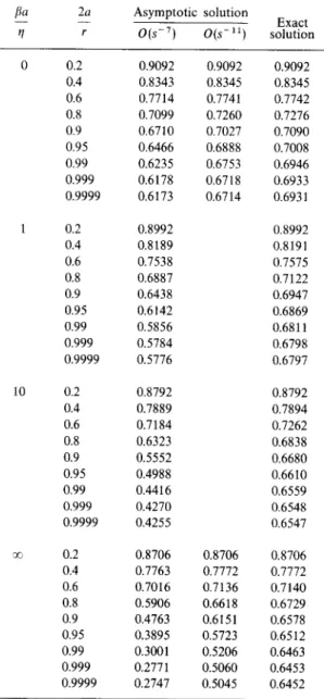
The exact (numerical) solution of the resistance functions x A 1 and )(A 2 was obtained by solving the problem of axisymmetric translational m o t i o n of two slip spheres using bipolar coordinates (Chen and Keh, 1995). Table 1 gives a comparison of our asymptotic solution from the m e t h o d of twin multipole expansions with this exact solution. F o r simplicity, only the

case of two identical spheres (al = a 2 = a and

[31 = [32 = [3) with equal velocities (U1 = U2 = Ue) is presented. In this specific case, the particles will ex- perience the same drag force (F1 = F2 = F) because xA1 = xA2 and )(A2 = xA 1. It is found from Table 1

that the predictions of ElF (°) [ = ( ) ( A l +)(la2)

([3a + 2q)/([3a + 3q)] from the asymptotic solution for

various values of fla/q are in g o o d agreement with

those of the exact solution. The errors in drag forces

Table 1. The normalized drag forces F/F (°) experienced by two identical spheres translating with equal velocities along

the line of their centers

fla 2a Asymptotic solution

-- - - Exact

r/ r O(s - 7 ) O(s -11) solution

10 0 0.2 0.9092 0 . 9 0 9 2 0.9092 0.4 0.8343 0.8345 0.8345 0.6 0.7714 0.7741 0.7742 0.8 0.7099 0 . 7 2 6 0 0.7276 0.9 0.6710 0 . 7 0 2 7 0.7090 0.95 0.6466 0.6888 0.7008 0.99 0.6235 0.6753 0.6946 0.999 0.6178 0.6718 0.6933 0.9999 0.6173 0.6714 0.6931 0.2 0.8992 0.8992 0.4 0.8189 0.8191 0.6 0.7538 0.7575 0.8 0.6887 0.7122 0.9 0.6438 0.6947 0.95 0.6142 0.6869 0.99 0.5856 0.6811 0.999 0.5784 0.6798 0.9999 0.5776 0.6797 0.2 0.8792 0.8792 0.4 0.7889 0.7894 0.6 0.7184 0.7262 0.8 0.6323 0.6838 0.9 0.5552 0.6680 0.95 0.4988 0.6610 0.99 0.4416 0.6559 0.999 0.4270 0.6548 0.9999 0.4255 0.6547 0.2 0.8706 0 . 8 7 0 6 0.8706 0.4 0.7763 0 . 7 7 7 2 0.7772 0.6 0.7016 0 . 7 1 3 6 0.7140 0.8 0.5906 0 . 6 6 1 8 0.6729 0.9 0.4763 0.6151 0.6578 0.95 0.3895 0.5723 0.6512 0.99 0.3001 0.5206 0.6463 0.999 0.2771 0.5060 0.6453 0.9999 0.2747 0 . 5 0 4 5 0.6452

(7)

Low-Reynolds-number are less than 1.8% for cases 2a/r <~ 0.6 if the asymptotic formula (31) is accurate to O(s -v) or less than 6.5% for cases 2a/r <~ 0.9 if eq. (31) is accurate to

O(s-1~). For the situation of two slip spheres with different radii, eq. (31) can also be found to agree well with the exact solution. In general, the accuracy of eq. (31) with finite terms decreases monotonically with the increase of fla/rl for a given value of s. In Section 5.1, one will see that the asymptotic results for the corresponding mobility problem of the same order of s-~ obtained from the same method are much more accurate than the resistance results presented here.

s = l / 1 +

{3

t

x - ~ Ps(~_~)(~_.) + s Q ~ _ ~ _ , ~ _ . i .

4.2. ~'A,(S, ) 0

We now consider two problems of the motion of two spheres normal to the line of their centers. In the first problem,

U 1 : - - U 2 : Ui (33) and in the second problem,

U1 = U2 = Ui (34)

with in each case ~ = ~"~2 = 0.

For the first problem, one has the coefficients in eq. (19) as

Zt~)n=(--1)'Ut~m~6nl, #l~)n=O, o~)n=O. (35a-c) In eq. (20), only the functions for m = 1 will be non- zero now. The expansions being used this time are "(" =(-1)=~2U ~ ~ P.pq P q tct t 3 - ~t (36a) / / I n p = 0 q=O n~. "~) = - i U Qnvq t , t 3 - ~t (36b) p=O q-O v , ~ ) = ( _ I ) ~ U ~ ~ 1 v q (36c) 1, p=O~=O 2n + 1

Vnpqt~t3-~"

The recurrence relations for coefficients P, pq, Q,v~ and V,p~, are

P.oo = 3 n l f 1 2 3 , Q.oo = 0 , Vno 0 = 3 n l f l O 3 (37a-c) and Pnpq ( n + l ) [ l + ~ n + 1 ) / 3 - 1 ] ~ : 1 n + l 2 n + l ( n + s ) ( n s + 4 ) - 2 ( n s + l ) 2 x fl2o2 n _ 1 2s(2s -- 1)(n + s) /1 >( Ps(q-s)(p-n+ 1) "~- ~ Ps(q-s)(p-n-1) n(2n + 1) -~- f120 - - ~/~(q -- s -- 2)(p -- n + 1) 2(2s + 1)

-- 23f12o(2n + 1)Q~a-~-l)~p-.+ll} (38a)

1795 (38b) n gnpq ~ Pnpq -- (n + 1)[1 + ( 2 n + 1)/~ -1 ] (n + s)(ns + 4) -- 2(ns + 1) z × Ps(q-s)(p-n+ 1) s(2s - 1)(n + s) 2 - (2n + 1)2/~ - ' - 2n + 3 P~(~-s)(v-,-1) (4n 2 -- l)l~- 1 + 2s + 1 Vs(q-s-2)(p-n+l) 4(4n 2 -- 1)/~-1Q~q_s_ 1)~v_.+1)],. (38c) 3 n

The force equation (21a) now leads to

I~(1-½(1 + ~)1~(2 = ~ ~ Plpqt~tg. (39)

p = 0 q = 0

By considering the second problem and comparing h A the result with eq. (39), it can be found that Y l l consists of the even powers of s and I2~2 of the odd powers of s. The explicit results can again be written as

Y A 1 = ~ . f 2 k ( , ~ ) ( 1 + ,~)-2ks-2k (40a)

k=O

Y~2 = - 2 ~, fzk+l(2)(1 + 2 ) - 2 k - Z s ~2k-1. (40b)

k=O

Here, fk(2) is given by the form eq. (32), and the first few values are

fo = flz3, f l = ~fl~32, f2 = 9 34fl232 f 3 = 2 f l O 3 f 1 2 3 , ~ _}_ 2 7 0 ' 4 8 / J 2 3 r" "[- 2 f 1 0 3 f 1 2 3 '~'3 2 2 ~L1./~ 5 ] 2 A = 6/~o~/~,~ + 1 6 v z ~ + 1 8 ~ o ~ , ~ ~ f 5 63/~ ~q3 ~ 2 2 4 3 /~6 ] 3 6 3 / 2 /~3 ] 4 = 2 / 3 0 3 P 2 3 ~" + 32 P 2 3 ~ -~- 2 /103/J23/~ f6 = 4 / ~ + 54Bo3/~h,~ ~ R 17~9- O 6 + , , ~ 64 , , ~ + 8/~o~);~ ~ + 81/~o~/~3;~ ~ 1 2 2 + 5 f 1 2 3 ( 3 f l f - 2 ) 3 + 20fl(_1~,, + 7 f 1 2 7 ) J , 5 fv ₌ is 3 _{5 f 1 2 3 ( 3 f l ( - 2 ) 3 +} _{20fl~-1~, +}_{7 f l 2 7 + 10flO2flO3),~ 2} D2 t 2 1 8 7 0 6 1 3 2 f l 2 3 ) , ~ 4 + x ° ~ # o ~ h ~ + ~ # h × ( 3 f l ( - 2 ) 3 + 2 0 f l ( - 1 ) 4 + 7 f l 2 7 + 1 0 f l o 2 f l o 3 ) J - 6.

(8)

1796 If/~ = 0, Jh = ~ ( - 4022 + 524 -- 8 0 2 6 -- 25627) J9 = ~ ( - 25622 - 8023 + 525 - 802~ - 2562s) J~o = ~ ( - 25622 - 8023 + 525 - 12027 - 512)fl - 128029 ) ft~ = ~ ( - 128022 - 51223 - 1202~ + 192526 - 1202 s - 51229 - 12802~°).

The above expressions are consistent with and much more accurate than the method-of-reflections results obtained by Hetsroni and Haber (1978) for the motion of two fluid drops (taking q* = 0) in the case fi = 0. F o r finite values of fi and r/*, the formulas of 2 A 1 , AA X~2, Y l l a n d *A Y12"A for the motion of two slip spheres and for the motion of two spherical drops are

identical up to

O(r -3)

if one puts fl = 3q*; however,

this is no longer true when terms of

O(r -~)

are re-

tained.

It can be found from eq. (40) that the interaction effect between two spheres translating perpendicular to the line of their centers is more significant when the slip coefficients at the particle surfaces become smaller (or when the value of/~ becomes larger). This behavior is consistent with that observed for the axisymmetric translation of two slip spheres.

4.3. ¢/~(s, 2)

The two problems specified in eqs (33) a n d (34) in the preceding subsection can be used to find functions Y~a(s, 2). Substituting eq. (36b) into eq. (21b) and ap- plying the definition of the resistance functions, one obtains

*B ¼(1 -~- /~)2flB 2 2 ~ ~ P q

Y I I -

=

Qlpqtlt2.

(41)

p=0 q-O

When the second problem is considered, it can be ~B

found that Y ~ consists of the odd powers of s and Y~2 the even powers. Thus,

flB1 = ~ f 2 k + , ( 2 ) ( l + 2 ) - 2 k - l s 2 k - I (42a) k-O Y~z = - 4 ~ fzd2)(1 + 2) -2k

es-~k.

(42b) k-O Here, k fk(2) = - 2 k+l Z O - k - q ) q 2q q=O

and some explicit expressions are

fo = A = o, J l = - 6/~o3/h32, .f~ = - 9/~o~/~132 2._7 ~ [~3 ~2 g - J4 ~ -- 2 /~03/J23 "~ ~A~/~ O4 .,2 f 5 = - - 1 2 f l g 3 f 1 2 3 2 - - 4 P03P'23 "; -- 36f123f12323 -- 72flo3f123 A

.fo = - 108fl~3fli322 - J~8 flo3f153)~3 2 2 .4

J7 = - 189B~3/~32~ - 3/~o~( ~ z ? ~ / ~ + 160/~o3/h5)23

-- 243f123f13324 --

48f123(6flo2flo5

+ 4/3(_ , , / ~ o 4 - 7/~o7)2 5.

It can be seen that ~B = 0 for all values of s in the limit/~ = 0. This is expected since the torques exerted on gas bubbles by the surrounding fluid are zero.

(43)

4.4.

)(C~(s, 2)

To determine the functions )(Cp(s,2), we consider two problems in which the two spheres rotate about the line of their centers. It is convenient to express the rotation in terms of a surface speed U:

a l ~ l = ~ aef12 = Ue. (44)

In each case, the translational velocities are zero (U~ = Uz = 0). When the minus sign is taken, the coefficients defined in eq. (19) become

Z~. = O,

~ . = O,

o ~ = 2U5,.o3.~.

(45a-c)

The only non-zero functions in eq. (20) are ~o.,"m which can be expanded as

-(~)

U

Q,pq

t~ t 3 - ~. (46)

"/On

p = 0 q = O

The recurrence relations for coefficients Qnpq are

Q.oo = 6.1flo3

(47a)

1 - - ,n --1,/~ -1

~ ( n + s )

Q"Pq=(n+l)[1

+ ( n + 2 ) / ~ 1]~=l n

X s Q s ( q s - 1)(p-n). (47b) After substituting eq. (46) into the torque equation (21b), one obtains

~ - c (1 + 2)33~c2 = ~ ~

Q,pqt~tq2.

(48)

8 2 p = 0 q = O

When the plus sign in eq. (44) is considered and its torque result is compared with the above equation, it is easy to find that

*c ~ f:,(2)(1 +

2)-ZRs :k

(49a) X l l k=O )(c a = - 8 ~ f2~+1(2)(1 +

2) -2k-%-2k-1

(49b) k=O where {01 i f k i s even fk(2) = 2 k Qltk-q)q2q+J' J = if k is odd. q=0 Explicitly, fo = / ~ 0 3 , f , = A = 0 f 3 = 8 i l L 2 3 , A = f s = 0 f6=64f13323, f T = 0 . If/~ = 0, Ac X ~ = 0 as expected. (50)

(9)

Low-Reynolds-number hydrodynamic interactions 4.5. ¢{ct~(s, 2)

The functions ^ c Y,o(s, 2) are obtained from problems

of two spheres defined by

a l ~ l = '}- a2~'~2 = U i (51)

with U~ = U2 = 0. W h e n the plus sign is considered, we have

Z~), = 0, ff~,) = 0, co~, ~ = ( - 1)'2Ufm16,~.

(52a~z) The expansions (36) a n d the recurrence relations (38) can be used again in this case, but the initial conditions (37) are replaced by

P, oo = O, Q,oo = 6,1flo3, 1/",oo = 0. (53a~z)

F r o m the torque exerted on a sphere given by eq. (21b) one finds

(1 -}- 2 ) 3 ^

yCll-~A

yc2

=

~ ~

Qlpqtlt 2.

Pq

(54)

p = O q = O

In the standard notation,

f c = i f2k(2)(1 + .~)-Eks-2k (55a)

k - O

}3c 2 = 8 ~ fek+1(2)(1 q- ,)~) 2k-'*s-2k-1. (55b)

k = O

Here,fk(2) is given by the form ofeq. (50), and the first few values are

fo = f103, f l = f : = 0 = = 18flO3f123,~ f3 = 4fl023 "~3, .[4 12flO23f1233~, f5 2 2 4 = 27flo3f123 z + 16f123(flo3 + 15fl25).~ 3 6 2 3 "2 ~l_A2 0 4 ] 5 ql_ 72flO33f12326. f7 = 72f133f123 '~4 + 2 /JO3P23 "~ Again, ~ c Y,~ = 0 in the limit/~ = 0.

5. T H E N O N - D I M E N S I O N A L M O B I L I T Y F U N C T I O N S

5.1. i~a(s, 2)

We now turn to the mobility functions 2aa(s, 2) a n d consider the external forces acting on the two spheres given by

(6~/al) 1F1 = - (6~qa2)- 1F2 = Ue (56)

where U is the magnitude of velocity that either sphere would have when the two spheres are far away from each other. In addition, there is no torque exerted on the spheres (T1 = T2 = 0). We wish to calculate the motion of the spheres, which is given by

U1 = Ule, U2 = - Uze and f l l = ~'~2 = 0. Similar to

the first problem considered for the resistance functions )f~a(s, 2), the quantities defined in eq. (19) for this problem are given by eq. (24) in which U is replaced by U,. Also, in eq. (20), only the functions p~.~ and v~, ~ with m = 0 are non-zero. The functions ,,(~)

_1"On,

v(') and the particle velocities U~ can be expanded as On

eq. (25) and

U~ = U ~ ~ Upqt~tq3_,. (57)

p = O q = O

F r o m eqs (21a), (25a) a n d (56) it is easy to know that

Plpq = 6pofiqo. (581

The recurrence relations for coefficients P, pq and V.pq

in eq. (27) remain valid. Taking n = 1 and using eqs (24), (25) and (57), eq. (20b) gives

~ s + l ~ " 3 p

Upq = = 1 ~ - ( - ~ s(q ~)p + flo2Ps(q-~*)(p- :,

+ ~ L(q-s-2)p (59)

which allows us to calculate the coefficients Upq from

using eqs (58) and (27). Using eqs (21a), (25a), (57) a n d (58), the mobility functions are related to these coefficients by

2)~ ~ .L

^ _ ^a = ~.~ Upqtltz.

X~l ~ x 1 2 ~ P " (60)

p = 0 q = O

Then, we consider the problem in which the forces are given by

(6rcqal)- IFI = (6ur/a2) 1F2 = Ue. (61)

It is easy to find that the velocities U, in this problem can be expanded in the form of eq. (57) with coeffi-

cients Upq being replaced by ( - 1)P+qUpq. Thus, a re-

lation between the mobility functions in the form similar to eq. (60) can be obtained.

As in the case of resistance functions, the mobility functions :~1 and :~z are given by a series either of even powers of s-1 or of odd powers,

2'~1 = ~ fZk(£)(1 + 2)-Zks 2k (62a) k - O 1 ~ )) 2~s_2k_ 2]2 = - - ~k__~0fZk+ 1(2)(1 + ~ , ~ (62b) where . ~ ( 2 ) = 2 k ~ q_j {~ if k is even q = O

U(k q)q)~

' J = if k is odd. (63) Explicitly, fo=f132, f 1 = - - 3 , . f z = 0 f3 = 4flo2(1 + 22), f4 = -- 60fl253~3, .fs = 0 f6 = 480fl05 )~3 -- ~(2fl(-3)2 -- 45fl05 + 63fl27)2 s f7 = -- 2400fl~5 )~3" If/~ = 0, fs = -- 38427, f9 = -- 2304( 23 + 25) flo = - 1536( 426 + 2 9 ) f l l = -- 6144( 223 + 325 + 227) •

(10)

1798

The expressions o f f s , f9, flo a n d fa ~ for the limiting situation of no-slip spheres (/~ ~ ~ ) can also be found in Jeffrey and Onishi (1984).

Using the so-called connector algebra, Geigenmul- ler and Mazur (1986) obtained the explicit formulas

for the mobility functions :~1,

)~2, Y~I

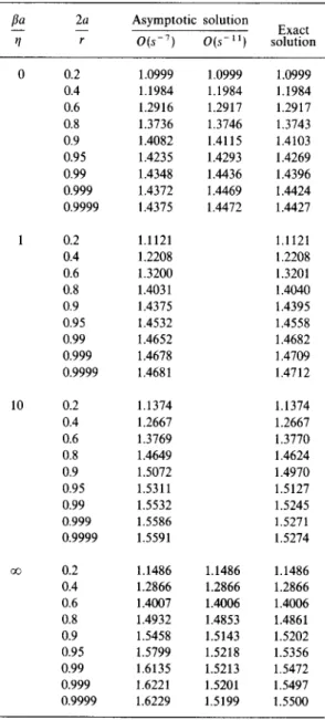
and .f~2 in

power series of 1/r up to O(r -v) for the case of two identical fluid drops. The above expressions agree with (and are more accurate than) their results (taking the viscosity of the drops as zero) for the case when /~ = 0. Again, the interaction between two slip spheres with a finite value of/~ can be found to differ from that between two fluid drops with a value of 3r/* equal to/~. The exact (numerical) solution of the mobility functions 2~1 and 2~2 for two slip spheres was also obtained by using bipolar coordinates (Chen and Keh, 1995). Table 2 gives a comparison of our asymptotic results with the exact solution for the case of two

Table 2. The normalized velocities U/U ~°) of two identical

spheres exerted by equal forces along the line of their centers

fla 2a Asymptotic solution

q r O(s -7) O(s -11)

identical spheres experiencing equal applied

forces (F1 = F2 = Fe). In this case, the particles will translate at the same velocity (U1 = U2 = U). It

is found in Table 2 that the predictions of U/U ~°J

[ = (x~l + x~2)(fla + 3q)/(fla + 2q), where U ~°) is the translational velocity of each particle subject to the applied force in the absence of the other particle] from the asymptotic approximation for various values of

fla/r l are in perfect agreement with those of the exact solution. The errors in velocities are less than 1.7% for cases 2a/r <<. 0.9 or 4.7% for cases 2a/r <~ 0.9999 if the

asymptotic formula (62) is accurate to O(s- 7). F o r the

situation of two spheres differing in size, eq. (62) can also be found to agree very well with the exact solution. Similar to the resistance problem considered in Section 4.1, the error of eq. (62) with finite terms is a m o n o t o n i c increasing function of fla/q for a given value of s. However, the results obtained from the method of twin multipole expansions for the mobility problem are much more accurate (and simpler in expression) than those (with the same order of s - 1 in the expansions) for the resistance problem. Thus, the

Exact better way to evaluate the resistance functions

solution through series expansions in s - 1 is to calculate the

mobility functions first and then use the reciprocal relations to determine the resistance functions.

0.2 1.0999 1.0999 1.0999 0.4 1.1984 1.1984 1.1984 0.6 1.2916 1.2917 1.2917 0.8 1.3736 1.3746 1.3743 0.9 1.4082 1.4115 1.4103 0.95 1.4235 1.4293 1.4269 0.99 1.4348 1.4436 1.4396 0.999 1.4372 1.4469 1.4424 0.9999 1.4375 1.4472 1.4427 0.2 1.1121 1.1121 0.4 1.2208 1.2208 0.6 1.3200 1.3201 0.8 1.4031 1.4040 0.9 1.4375 1.4395 0.95 1.4532 1.4558 0.99 1.4652 1.4682 0.999 1.4678 1.4709 0.9999 1.4681 1.4712 10 0.2 1.1374 1.1374 0.4 1.2667 1.2667 0.6 1.3769 1.3770 0.8 1.4649 1.4624 0.9 1.5072 1.4970 0.95 1.5311 1.5127 0.99 1.5532 1.5245 0.999 1.5586 1.5271 0.9999 1.5591 1.5274 0.2 1.1486 1.1486 1.1486 0.4 1.2866 1.2866 1.2866 0.6 1.4007 1.4006 1.4006 0.8 1.4932 1.4853 1.4861 0.9 1.5458 1.5143 1.5202 0.95 1.5799 1.5218 1.5356 0.99 1.6135 1.5213 1.5472 0.999 1.6221 1.5201 1.5497 0.9999 1.6229 1.5199 1.5500 5.2. 9a,(s,,~)

We now consider the motion of two spheres perpendicular to the line of their centers, and again define two problems. First

(6nqax) 1F1 = - - ( 6 n q a 2 ) - l F 2 = Ui (64) and, secondly,

( 6 n r / a l ) - l F 1 = ( 6 n q a 2 ) - l F 2 = Ui (65) with in each case T1 = T2 = 0. The purpose is to find the translational velocities UI = U l i and U2 = -T- Uzi as well as the angular velocities f~l = - f l l j and ~ z = -T- ~2J.

F o r the first problem, the coefficients defined in eq. (19) become

Z~)n = (--1)3-~Ua6m1~nl, ~l~n = O,

~,~, = 2a, fft,6,,t 6,1. (66a-c)

The quantities p~,), q~,J, V~l~, ), U, a n d ~ , can be expanded as = P,pq ta t3 - a (67a) p = O q = O q(x~,~ = iU ~ ~ Q,pqt:t~_~ (67b) p = O q = O 2n + 1 V"vqt't3-" (67c) U~ = ( - - 1 ) 3 - a U ~ ~ Uvq,,,a'v:_, (68) p=Oq=O a ~ = U ~, ~ I) ,v,q pq~at3-at. (69) p = O q = O

(11)

Using eqs (21), (64) and (67a,b), one finds

Plpq = 6pofqo, Qlpq

= 0. (70a, b)

All coefficients

V,pq

are calculated from the relation

V.pq

( n + l ) [ l + ( 2 n + l ) / ~ - t ] ~ = ~ + 1

!n + s)(ns +

4) -

2(ns +

1) 2

X Ps(q s}(p

n+l)

n(2n +

1) q- /?l

210---'~)

+ - - ~ ( 2 n - - 1 ) Q ~ l q ~ l ~ t p - . + l ~

n ( 2 n -

1) 1 + 2(2s + 1~ V~(q-~-2)(p-,+ 1)~ +

6,~/?oaUpq.

(71) For n > 1, the recurrence relations for coefficients P.pq and

Q.pq

are given by eqs (38b,c). Substitution of n = 1 into eqs (20b,c) using eqs (66) and (67) gives expressions for coefficients

Up~

and ~p~:

U~q = ~ s(s + 1)~_ 3(s_~_2_) s= 1 2 14s(2s - 1) Ps(q-sip 1 - - a / ? o z P s ( q - s l ( p - 2) -]- Q s ( q - s - 1)p 4(2s + 1)

V~(q-~-2)p

(72a) 3 p f~pq= ~=,~ s ( s + 1 ) { ~ s ( q - s ) ( p - 1 )

sQstq-s-~)(p-~)}.

(72b) The coefficients

Upq

are related to the mobility functions by

~ - ~ = ,.., ( - 1 ) Upqtlt 2. (73)

p = 0 q = 0

When the second problem is considered and its result is compared with eq. (73), one has

)"~ 1 = ~ f2k(~-)( 1 ~- 2) - 2ks - 2k (74a)

k 0

33'~2 = ½ ~ ./~k+l(2)(1 +

2)-2ks -2k-~

(74b) k=O

wherefk(2) is given by eq. (63) and the first few values a r e fo=/732, f ~ = 3 f 2 = O A = 2 / ? o : 0 + ,~), f , = f ~ = o f6 = - ~s(4/?~-3)2 + 60/?(_ ~,, + 21//27)25, f7 = O. I f / ~ = O,

f s = 3 ~ s 27, ,[9=0,

f a o = 3 8 4 2 9 , f ~ , = 5 7 6 2 s.

Again, these formulas are consistent with and more accurate than the results obtained by Geigenmuller and Mazur (1986) for the motion of two identical fluid drops (taking r/* = 0) in the limit/~ = 0. Similar to the resistance problem, the expressions of 2 a , .~AE, )3~1 and 33A2 for the motion of two slip spheres and for the motion of two spherical drops at finite values of /~ and r/* are identical up to O(r -3) if one puts /~ = 3q*; the difference between them appears when terms of O(r 4) are included.

5.3. ~2~(s, ;3

The calculations in the preceding subsection can be used to find functions

)3~t~(s,

2). The coefficients f~pq in series expansion (69) for the angular velocity of a sphere translating under an applied force are given by eq. (72). The functions )3~a are then deduced in the standard way with the difference that odd powers of

^b

s i in the series go to Yll and even powers to )3~2. The result is fi bll = 2 f 2k+1(2)(1 q- ~ ' ) - 2 k - l s - 2 k - 1 (75a) k=O

33~2 = ¼ ~ fzk(2)(1 +

2)-2k+2s 2k. (75b) k=O Here

fk(2)=(2)k ~ f~k-q,o 2q j,

j = { ; i f k i s e v e n o=o if k is odd, (76) and some explicit expressions are

fo = A = o, J i = - 2, f3 = f 4 = J'; = f~ = 0 fv = 160fl0523 + 16(6/705 + 4/? I- 1)4 - 7/?27) 25. 5.4. ~p(s, 2)

In order to determine the functions ~a(s,2), we consider the torques acting on the two spheres given by

(8nqa3)-lT1 = -T- (8nt/a3)-lT2 =f~e. (77)

Because the translational velocities are zero (given F~ = F2 = 0), the only non-zero functions in eq. (20) are q~2. When the minus sign in eq. (77) is considered, q ~ can be expanded as eq. (46) and the particle angular velocities can be expressed as eq. (69) with U being replaced by a~ f~ now. By the combination of eqs (20c), (21b) and (69), the coefficients

f~pq

are obtained from the relation

f~q =/?30Qlpq - S(S

+

1)

s = o 2

Q.~lq -~

- 111~ - ~1. ( 7 8 )

The recurrence relation for coefficients Q,pq is given by eq. (47b) with the initial value Q,oo = 6,x. Using eqs (21b), (46), (69) and (78) and observing that the even and odd powers of s-x in the series go to the functions 2~1 and ~ 2 , respectively, one

(12)

1800 obtains x ] l = ~ f2k(2)(1 +

2)-2ks-2k

(79a) k = 0 212 = - s 1 ~ f2k+l(2)(1 +

2)-2k+2s -2k 1

(79b) k = 0 where ~, ' {02 if k is even (80) f k ( ' ~ ) =

~(k-q)q'~'q-J'

J = if k is odd. q=O Explicitly, To = / h o , f~ =f~ = 0 f 3 = l ,

f , = fs = f6 = fT = O.

Note that x~t --* o% as expected, and x~2 = - 18s-3 in the limit/~ = 0.

5.5. ~e(s, 2)

The functions ~3~,a(s, 2) are to be obtained from problems of two spheres in the situation that

(8zr/a~3) - 1T 1 = _+ (8~rqa3) T M 1T 2 = f2i (81)

with F I = F2 = 0. The recurrence relations used to calculate ~ p in Section 5.2 with U being replaced by a,fl can be used here with only a change of initial conditions,

Plvq = O, Qlpq

= 5pO6qO,

Vlp q

= 0. (82a-c) As usual, we have Y~I = ~ f2k(~.)( 1 + ~,) -2ks-2k (83a) k=O 1 oc ~') - 2 k + 2 S - 2'k- 1"

Y]2 = ~k~=of2k+

1(2)(1 + (83b)

Here,fk(2) is given by the form ofeq. (80), and the first few values are

/o=/ho, /~=/~=0, A = - 4 , / , = / ~ = 0

f 6 = - - 2 4 ( f l o a + 9 f l 2 5 ) "~3, f7 = 0. As expected, ~ t l ~ oo in the limit/~ = 0.

6. A V E R A G E S E T T L I N G V E L O C I T Y I N A S U S P E N S I O N O F S L I P S P H E R E S

In practical applications of sedimentation phenomena, collections of particles in bounded systems are usually encountered. The interaction effects between pairs of spheres discussed in the previous section can be used to find how the average settling (or buoyantly rising) velocity of a dilute suspension of slip spheres is affected by the volume fraction of the particles. Based on a microscopic model of particle interactions in a dilute dispersion which comprises both statistical and low Reynolds number h y d r o d y n a m i c concepts (Batchelor, 1972; Reed and Anderson, 1980), the average settling velocity of a test particle (with radius a,), which samples all positions in a bounded

dispersion, is given by ( U ' ) = U I ° ) + C { f v v * ( r ) [ o ( r ) - l ] d r + ~ . J r > a V2 v*(r) [g(r) -- 1] dr ~_ 2 a 1)U(O) -+- 37zat a ( 2 f 1 2 3 - -

+ f v W(r)g(r)dr} +0(C2)"

(84)

Here, C is the macroscopic concentration of the neighboring particles (assumed to be identical, with radius a), Ut, °J and U (°) are the undisturbed settling velocities of the test particle and a neighboring particle, respectively, g(r) is the two-particle radial distribution function, and V denotes the entire volume of the dispersion, v*(r) is the velocity field at position r when a single neighbor particle at the origin 0 moves with velocity U <°), which can be expressed as (Basset, 1961)

r < a: v*(r) = U (°) (85a)

(85b)

The Laplacian of this field can be found to be

r < a: V2v*(r) = 0, (86a)

r > a: V2v*(r) = ~fl23 [I - 3 e e ] . U (°). (86b) W(r) in eq. (84) is a correction function needed to account for the perturbation on v* owing to the pres- ence of the test particle and the boundary, and is given by

W(r) = U * ( r ) - UI °) - v*(r) - 61flo2a2V2v*(r) (87) where U*(r) is the actual velocity of the test particle located at r with respect to the origin of a single neighbor at 0. If all the particles have the same value of /~, U*(r) can be calculated using the mobility functions derived in Sections 5.1 and 5.2,

U*(r) = [2~1U~ °) + 22 ~. U(O)]. 1 + 2 12 j e e

+ [;~lul °, +--L-2 "'~ u(°']/

1 + ,l y12 j.(I e e ) (88)

where subscripts 1 and 2 denote the test and neighboring particles, respectively. Substitution of eqs (85b), (86b) and (88) into eq. (87) shows that the magnitude of W behaves as r - 4 when r >> a.

The volume integrals in eq. (84) can be evaluated by assuming that the radial distribution function has the

(13)

Low-Reynolds-number following equilibrium value for rigid spheres without long-range pair potential:

g = 0 if r < a, + a (89a)

g = 1 + O(C) i f r > a, + a (89b) where O(C) is a term p r o p o r t i o n a l to the concentration of the neighbor particles. That is, the particles must be sufficiently small so that Brownian motion dominates any multiparticle h y d r o d y n a m i c interactions which might impart microscopic structure to the dispersion. In general, it is necessary to obtain the pair distribution function as the solution of a conservation equation of the F o k k e r - P l a n c k type for a polydis- perse system of spheres (Batchelor, 1982). The conditions under which the assumption of local equilibrium is valid for a dilute dispersion comprising different types of particles are also discussed by Reed and Anderson (1980).

Given eqs (85)-(89) and the relation U ~°)

= UI, °) ae/a 2 (assuming that the test particle and its neighbors have the same density), the integrals in eq. (84) can be evaluated to yield

<Ut> = UI°)[ -l -~- ~t~ "}- O(~92)] (90) with 15 a 1 -- --f123(4fl( 3)2 -F 20fl~-1)4 - 60flo5 4O ata 2 75 2 ata3 + 9 1 f l 2 7 ) ~ + -~f123flZ5ia;~_a)4 (91)

where q~ ( = 4rca 3 C/3) is the volume fraction of the neighbor particles. N o t e that the integral of the modi- fied F a x e n correction involving V2v * (Felderhof, 1976) in eq. (84) equals zero as computed from eqs (86b) and (89). The term inside the brackets in eq. (91) for ~, is obtained from the first and third terms in the braces of eq. (84), while the other terms in eq. (91) are the result of the last integral in eq. (84). Certainly, this expression is not exact, even given that eq. (89) holds, because O(r-s) terms are neglected in the evaluation of U * ; however, the error should be small and will a p p e a r only in the calculation involving the correction function W. In the derivation of eq. (91), all the neighboring particles are assumed to be identical, even though they are allowed to differ in radius from the test particle.

F o r a dispersion of particles that have a distribution in radius, a generalization of eqs (90) and (91) leads to

(Ui> = U,°)[1-4- 2 o~ij~oj-t'- O((02)] (92) J hydrodynamic interactions where O~ij = -- 1 + 3fl2 3 ~// + \ai,] d 15 / a i \ 5 / ai ~3 1 40f123(4fl~ 3}2 Jr- 20fl(-1) 4 -- 60flO 5 aia } 75 2 aia3 + 91f127)(a, + aj)3 I- ~ f 1 2 3 f 1 2 5 i a ~ a j ) 4. (93) Here, subscript i denotes the type of particles having radius a~. Note that eqs (91) and (93) are valid only when all the particles have the same density and value of/~.

An examination of eq. (93) indicates that the interaction coefficient ~ i is always negative, irrespective of values of aj/a~ and/~. Thus, the average settling velocity of a type of particles is reduced with an increase in the concentration of any type of particles in the suspension. Results of ~ j calculated from eq. (93) at various values of aj/a~ are plotted vs/~ in Fig. 1. It can be seen that, as expected, the magnitude of ~ij, which reflects the intensity of particle interactions, increases monotonically with the increase of/? for a fixed value of aHai. If the value of/~ is kept constant, the magnitude of e~j is a monotonic increasing function of the ratio aj/ai. Namely, the influence of the interactions on the smaller particles is stronger than on the larger ones. Note that, in the limit aj/a~ = 0, eq. (93) predicts that e~j = - 2 for the case of/3 = 0 and % = - ~ [if more accurate values of the mobility functions in eq. (88) are used, ~ j = - 2 ~ as indicated by eq. (94)] for the case of/~ --, o~.

F o r a suspension of no-slip spheres (/~--, ~ ) , the mobility functions in eq. (88) can be calculated to the order of r - 11 (Jeffrey and Onishi, 1984); thus, a more accurate expression for :qj than eq. (93) is obtained,

O ~ i J = - - I l+3aj-ai + \aij(aJ~2~] -- 415 ( ai ~\~/i

5 f a i "~3 11 aia } 75 aia 3

+ ~ k ~ / I I 8 (ai + aj) ~ 3 + 16(ai + aj) 4

5 ( a, ~5 15 ai3 2aj 9 aia~

4 k ~ / + 4 (ai + aj) 5 10 (ai + aj) 5

5 2

3 3 5 ai@ 35 a~aj

5 a i aj

8 (a i -l- a j) 6 8 (a i -+- a j) 6 8 (a i -}- tlj) 7

375 _{al aj}4 3 21 _ai3 4 _aj 9 aia 6 28 (ai + aj) 7 4 (ai + aj) ~ 14 (ai + a j) 7

25 a.5, a 3 4177 a3@ + + 8 (ai+aj) 8 25 aiaJ 8 ( a i + a j ) 8" 256 (ai + a j) 8 (94)

(14)

1802 H.J. Keh and S. H. Chen 12 10 8 --O~ij 6 4 2 0 . 5

~

" 0 . 2 o I I i I I I I

Log /~

Fig. 1. Plots of coetficient ~j calculated from eq. (93) for a bounded suspension of slip spheres vs/~ with aj/a~

as a parameter.

Similarly, for a suspension of perfect-slip spheres or spherical gas bubbles (/~ = 0), ccij can be evaluated by the following formula of the same accuracy:

~ij=__[1..~ -

2(lj_~_(flj)21 ai 1 aia 2 al \ a i / A ai + aj 4 (al + aj) 3

1 aia 3 3 aia~ 1

a i3

a j3 t-

2 (al + a j) 4 25 (ai + aj) 5 2 (ai + aj) 6

1 aia~ 4 a i4 a j3 1 aia 6 2 (al + aj) 6 7 (ai + aj) 7 14 (a i + aj) 7

1 a~a 3 51 a i3ajs 1 aia]

2 (ai + ay) ~ + 64 (ai + a j) ~ + 2 (ai + aj) s" (95) +

To our knowledge, analytical expressions for ~ij analogous to eqs (94) a n d (95) have never been derived before.

When all the particles in the dispersion are identical, eqs (92) a n d (93) reduce to

<U> = U¢°)[1 + ~o + O(~oZ)] (96)

= - (2 + 3//23) - 8L'5-f123f125 ± -- 320f123(4fl(- 3)2 + 20fl~_ 1)4 - 160flo5 + 91fl27) + 75rc256/J23/~25 . 0 2 (97) O n the other hand, the average settling velocity in a suspension of identical fluid drops can be determined in the same procedure using the connector- algebra results for 2~1, 2~2, J311 a n d j3] 2 accurate to

O ( r - v ) obtained by Geigenmuller and M a z u r (1986).

The coefficient ~ for this case is 4 + 5 q * ( 2 + 3 r / * ) ( 2 + 5 q * ) 1 + q* 8(1 + r/*) a 24 + 55q* - 144q .2 - 27q .3 192(1 + q*)/(4 + q*) (2 + 3r/*)(2 - 5q*) 2 -~ 256(1 + q,)3 (98)

In eqs (97) and (98), all terms except the first one are the contribution from the integral involving the correction function W. It can be found that eqs (97) and (98) are equivalent for the limiting cases of a suspension of no-slip particles (/~ --, ~ , q* ~ ~ ) and of perfect-slip bubbles (/~ --* 0, q* ~ 0).

The accuracy of the value of c0 in eq. (96) depends on the accuracy of W(r) defined by eq. (87) or U*(r) given by eq. (88) being used in the calculation. Table 3 lists the results of ~ for the limiting cases of/~ ~ ~ and /~ = 0 when the mobility functions 2~1, X~Z, J ~ l a n d 3~] z in eq. (88) are calculated to various accuracies of

order of r -1 from O(r -3) to O(r -11) using eqs (94)

and (95). All the previous calculations of u for a suspension of identical solid or fluid spheres in these limits using numerical solutions for the mobility functions are also given in this table for comparison. It can be seen that the convergence of our results of c¢ is not perfect yet even if the accuracy of O(r-11) is achieved; nevertheless, the agreement between these results and those predicted by Batchelor (1972), Reed a n d Anderson (1980) a n d Keh a n d Tseng (1992) is quite good.

(15)

Low-Reynolds-number hydrodynamic interactions Table 3. The results of coefficient a defined by eq. (96) for

a suspension of identical spheres for the limiting cases of no slip ( / ~ ~ ) and perfect slip (/~ = 0)

Accuracy of the - mobility functions used in eq. (88) /~ --, oo /~ = 0 O (r- 3 ) 5.000 4.000 O(r 4) 6.875 4.500 O(r 5) 6.875 4.500 O(r 6) 6.734 4.531 O(r- 71 6.441 4.500 O(r -8) 6.391 4.504 O(r -9) 6.411 4.488 O(r -1°) 6.514 4.493 O (r- 11 ) 6.553 4.486 Batchelor (1972) 6.55 ---

Reed and Anderson (1980) 6.53 4.54

Keh and Tseng (1992) 6.49 4.44

7. CONCLUDING REMARKS

In this work, an analytical study for the slow motion of two slip spheres in an infinite fluid is presented using a method of twin multipole expansions. The spheres may have different radii and arbitrary translational a n d rotational velocities (or applied forces a n d couples). The resistance and mobility functions that relate the forces and couples to the translational and rotational velocities have been derived in Sections 4 and 5 in the form of power series of s - t, where s is the dimensionless distance between the centers of the spheres defined by eq. (8a). The presented results include the hydrodynamic interactions between two no-slip spheres a n d between two perfect-

slip spheres (spherical gas bubbles) as special cases. It a

is found that the particle interaction effects decrease a, b, ~ e

with the increase of the slip coefficients at the particle A, B, B, C

surfaces. Ying and Peters (1989) also used the twin C

multipole expansion method to treat the problem of

the fluid dynamic interactions of two spheres in e

a slightly rarefied gas. In their analysis, the b o u n d a r y

condition applied at the particle surfaces was deter- e~

mined from a perturbation expansion of the linearized F

Boltzmann transport equation for the gas molecules.

Their results for the resistance and mobility matrices 9

of the two-sphere system were obtained at small but

finite K n u d s e n numbers and shown to recover Jeffrey I

and Onishi's (1984) solution when the K n u d s e n i, j, e

n u m b e r is zero.

O u r solution for the interactions between pairs of p

spheres has also been utilized to calculate the mean pro,, q,,,, vm,

settling velocity in a b o u n d e d dispersion of slip r

spheres. An analytical expression of this mean velocity

in the general case is given by eqs (92) and (93). F o r the r

limiting cases of no slip a n d perfect slip at the particle r,, 0,, ~b surfaces, our results, expressed by eqs (94) a n d (95)

respectively, are found to agree well with the numer- s

ical solutions available in the literature. The mean t

settling velocity is always reduced as the concentra- T

tion of particles in the suspension is increased. Again,

this effect of retardation is less significant if the slip coefficients at the particle surfaces are increased.

The general construction of the resistance a n d mobility relations for the motion of two rigid spheres involves the forces, torques, and stresslets exerted by the spheres on the fluid, and the translational and angular velocities of the spheres in the ambient velocity field U(x) = Uo + f~ x x + E. x, where E is a constant rate-of-strain dyadic (Kim a n d Mifflin, 1985; Kim and Karrila, 1991). Thus, the complete (grand) resistance and mobility matrices are 6 x 6 matrices of tensors of second, third and fourth ranks. The axisym- metry a b o u t the axis through the sphere centers implies that each tensor can be decomposed into an expression involving no more than three scalar functions. Using the consequences of the stresslets and E being symmetric and traceless, the reciprocal theorem and the two-sphere symmetry, it can be shown that there will be another 12 independent scalar functions (in addition to the 10 functions considered in Section 2) to be determined for either a resistance problem or a mobility problem. F o r the special case of two no-slip spheres, these 12 resistance functions were calculated using the method of twin multipole expansions by Jeffrey (1992). This analysis can be extended without difficulty to the general case of two slip spheres.

Acknowledgement

This research was supported by the National Science Council of the Republic of China under Grant No. NSC84- 2214-E002-006.

NOTATION particle radius, m

mobility tensors defined by eq. (11) resistance tensors defined by eq. (4) n u m b e r density of particles in suspension, m 3

unit vector pointing from particle 1 to particle 2

unit vector in the direction of r~ force exerted by a particle on the fluid, N

two-particle radial distribution function

unit dyadic

unit vectors in rectangular coordinate system

dynamic pressure, N m - 2

coefficients defined by eq. (18), m s 1 vector pointing from particle 1 to particle 2, m

equal to I r], m

spherical coordinates with respect to particle

[ = 2r/(al + a2)] ( = a/r)

torque exerted by a particle on the fluid, N m