5~6 GHz頻段室內寬頻／超寬頻無線通道量測與模擬(III)

行政院國家科學委員會專題研究計畫 成果報告

5～6 GHz 頻段室內寬頻／超寬頻無線通道量測與模擬(3/3)

計畫類別： 個別型計畫

計畫編號： NSC93-2213-E-009-020-

執行期間： 93 年 08 月 01 日至 94 年 07 月 31 日

執行單位： 國立交通大學電信工程學系(所)

計畫主持人： 唐震寰

報告類型： 完整報告

報告附件： 出席國際會議研究心得報告及發表論文

處理方式： 本計畫可公開查詢

中 華 民 國 94 年 11 月 4 日

5~6 GHz 頻段室內寬頻／超寬頻無線通道量測與模擬(3/3)

5~6 GHz Wideband / Ultra-wideband Radio Measurement and

Channel Modeling for Indoor Environments (3/3)

計畫編號：NSC93-2213-E009-020 執行期限：93 年 8 月 1 日至 94 年 7 月 31 日 主持人：唐震寰 國立交通大學電信工程學系 中文摘要 超寬頻無線技術由於其高傳輸容量、不易受多重 路徑影響、具備精密的定位及測距能力、以及不易 被截取等優點，近年來在科學、工業、通信及軍事 等領域上都獲得相當大的重視，歐美各國也都相繼 投入其應用研發。為瞭解超寬頻信號在室內的通道 特性，本計畫乃規劃以掃頻量測方法，量測及探討 其室內傳播特性。本計畫將於三年內進行兩階段之 研究工作： (1) 第一階段(第一及第二年)：對超寬頻 信號傳播路徑損耗、衰落、及功率延遲分佈等特性 進行量測與模型建構及驗證；(2) 第二階段(第三 年)：以第一階段的研究結果應用於在探討超寬頻信 號在室內無線傳播特性。 在計畫執行的第一年中，我們完成了超寬頻室通 道量測系統的架設，以此系統對5 ~ 6 GHz 寬頻信號 在室內的傳播特性進行量測。同時，也以所發展的 三維適應環境性傳播模型及射線追蹤技術來模擬此 一頻段的無線信號在室內環境的傳播現象。為能獲 得較合理的模擬結果，研究中同時也對一般室內建 材在超寬頻頻段的介電係數進行量測，並將所測得 的介電係數用於模擬中。經比較量測與模擬所得的 數據，証實了此傳播模型之有效性與正確性。 計畫執行的第二年，我們以預估延遲拍線模型為 基礎，對室內超寬頻信號功率延遲分佈的相關參數 如時間延遲係數和功率損耗率等進行分析。同時也 推導出時間延遲係數和功率損耗率與信號頻寬的關 係式，可用以預測室內環境中不同頻寬信號的功率 延遲分佈特性。研究中也以所架設之超寬頻脈衝響 應量測系統，在不同條件的室內環境下進行了大量 的量測。經與量測結果比較後，也驗證了所推導模 型的正確性，並且得到兩項結果：(1) 同一傳播環靜 中，信號的頻寬並不會對平均功率延遲分佈的時間 延遲係數造成影響；(2) 同一傳播環靜中，平均功率 延遲分佈的功率損耗率會隨著信號頻寬的增加而減 少。 本年度為計畫的第三年，我們藉由 Stochastic tapped-delay-line（STDL）模型，完成室內超寬頻無 線通道參數隨頻率變動之公式推導。該模型利用衰 減常數（delay constant）、電功率比值（power ratio） 及Nakagami 常數描述通道特徵。如給定窄頻通道特 徵參數值，可利用上述公式計算超寬頻通道特徵參 數值。該研究成果經與在實驗室、辦公室及教室內 大量實測結果（3GHz~5GHz）驗證，顯示良好之預 估準確性。實測結果同時顯示通道特徵參數與頻寬 之關係：（1）電功率比值隨著頻寬之增加而變大；（2） 衰減常數與頻寬似乎無關；及（3）Nakagami 常數也 隨著頻寬之增加而變大。 整體而言，感謝國科會之研究補助使本多年期研 究計畫得以順利執行並完成。目前已投稿一篇IEEE Trans. on Vehicular Technology（under revised）、一篇

IEEE Trans. on Wireless Communications，以及數篇國 際會議論文。

關鍵詞：超寬頻、無線電傳播、通道響應、STDL 模 型、頻寬效應

Abstract

Ultra Wideband (UWB) radio techniques have recently attracted great interest in scientific, industrial, commercial, and military sectors. The potential strength of the UWB radio technique such as high channel capacity at short range, lack of significant multipath fading, accurate position location and ranging, and extremely difficult to intercept, lies in its use of extreme wide transmission bandwidths.

In this project, a spectrum analyzing and a swept frequency measurement methods are adopted to measure and to analyze the UWB radio propagation loss, multi-path fading, signal delay and spread. It is a three years project and is separated into two stages. (1) The first stage (1st and 2nd years): measurement and modeling of the UWB radio propagation loss, multi-path fading, and power delay profile; (2) The second stage (3rd year): investigation of UWB indoor propagation characteristics.

In the last annual report, an ultra wideband channel sounding system and a swept frequency measurement method are adopted to measure and to analyze UWB radio wave propagation characteristics in indoor environment. A site-specific model using ray-tracing technique is developed to predict the radio propagation in indoor environments. Simulation results are validated by the experimental results.

In the second year, the stochastic tapped-delay-line (STDL) model is introduced to model the UWB indoor channels with the parameters, delay constant and power ratio, of the averaged power-delay profile (PDP). Here, the formulas of these two parameters versus signal bandwidth are proposed. The formulas have been validated by comparing the computed results with a large number of measurement data carried out at many sites such as classrooms, laboratories and offices. The measured frequencies are ranged from 3 GHz to 5 GHz. It is found that (1) The delay constant of the averaged PDP is independent of radio bandwidth; (2) The power ratio of the averaged PDP is decreased when the

radio bandwidth is increased.

In the third year, modeling dependency of Ultra-Wideband (UWB) indoor radio channel parameters on bandwidth is explored. Here, formulas describing these dependencies are derived under the stochastic tapped-delay-line (STDL) model, which characterizes radio channels using parameters such as decay constant, power ratio and Nakagami parameter. Through these formulas, the proper UWB channel parameters for a ultra-wide bandwidth signal can be determined from those of a narrow bandwidth signal. These formulas have been validated by comparing the computed results with a large number of measurement data carried out at laboratories, offices and classrooms. The measured frequencies are ranged from 3 GHz to 5 GHz. It is found that (1) The power ratio is decreased when the signal bandwidth is increased; (2) The decay constant is independent of radio bandwidth; and (3) The Nakagami parameter is increased as the signal bandwidth is increased.

As a whole, with these research achievement, we had submitted one paper to IEEE Trans. on Vehicular Technology (in revised), another paper to IEEE Trans. on Wireless Communications, and some presentations at international conferences. Keywords: UWB, radio propagation, channel

impulse response, STDL model, bandwidth effect.

I. Introduction

Ultra-Wideband (UWB) radio techniques have recently attracted great interest in scientific, industrial, commercial, and military sectors. The potential strength of the UWB radio technique such as high channel capacity at short range, lack of significant multipath fading, accurate position location and ranging, and robustness to interception, lies in its use of extreme wide transmission bandwidths [1]. According to the Federal Communication Commission (FCC) regulations of UWB radio technology and systems [2], the minimum bandwidth limit of an UWB radio signal is 500 MHz, and the frequency band from 3.1 GHz to 10.6 GHz is available for unlicensed use for indoor communication applications. Due to its extremely wide bandwidth, each UWB system achieves very high resolution in the delay domain. Therefore, the UWB channel response may contains several tens to hundreds multipath components (MPCs), which are very different from those of conventional narrowband/ broadband indoor wireless communication systems. Therefore, precise multipath models are of primary importance to the UWB channel models.

It is noted that for band-limited radio systems, the signal resolution, proportional to the

inverse of the bandwidth, affects the number of resolvable MPCs and their powers, and of course changes values of the channel response parameters as well. It is important to find the dependency of channel parameters on signal bandwidth for UWB radio systems since their signal bandwidth may vary in a wide range to provide manifold applications with varying data rate and quality of services requirements. In theory, channel responses of narrowband signals may be derived from that of wideband signals by a simple bandpass filtering operation, but it is difficult to estimate the channel responses of any wideband signal from those of a narrowband signal.

In this paper, modeling dependency of UWB indoor radio channel parameters on bandwidth is explored. Here, the formulas describing these dependencies are derived under the stochastic tapped-delay-line (STDL) model [3], which characterizes radio channels using parameters such as decay constant, power ratio and Nakagami parameter. Through these formulas, the proper UWB channel parameters for a wide bandwidth signal can be determined from those of a narrow bandwidth signal.

This paper is organized as follows. In Section II, the STDL model that we adopted to characterize the indoor UWB radio propagation channel is presented. The dependency of channel parameters on bandwidth are analyzed and derived in Section III. In Section IV, the measurement system and environments are described. Results of our finding are validated by measurement data in Section V. Conclusions are given in Section VI.

II. The STDL Channel Model

Because of multipath propagation due to reflections, refractions, and/or scattering by obstacles or scatters in propagation environments, radio propagation channels are usually modeled as a linear filter with a complex-valued lowpass equivalent impulse response that is expressed as

( )

=

_∑

(

−

)

k k k

a

h

τ

δ

τ

τ

(1)

where ak and τk are the random complex-valued path gain and propagation delay of the MPCs, respectively; and δ is the Dirac delta function.

To characterize the statistical properties of UWB indoor channels, the STDL model was proposed by Win et al [3]. It characterizes the shape of the power delay profile (PDP) of the UWB indoor channel in terms of power gains and delays of taps, i.e, by the pairs {Pi, τi} with

τi=(i-1)×∆, where ∆ is the tap spacing and is

system. Meanwhile, Pi is equal to the square of

the vectorial sum of the arriving MPCs over a tap spacing beginning at the delay (i-1)×∆ , i.e., Pi= | Σ ak|2, for (i - 1 ) ×∆≦τk < i ×∆.

In the model, the small-scale averaged PDP,

( )

τ

P , is modeled by a single exponential (linearly

on a decibel scale) PDP with a stronger first tap as shown in Fig. 1 and is expressed as

( ) ( ) ∑ ( ) ⎟ ( − − ×∆) ⎠ ⎞ ⎜ ⎝ ⎛₋ − ×∆ + = = ( 1) 2 exp 2 i i r P L i τ δ ε τ δ τ (2)

where L is the total number of taps in the observation window, ε is the exponentially power decay constant and r is the power ratio that is defined as the ratio of the averaged power of the second tap to the first tap, i.e, r=P₂ P₁. It is

noted that, P_i is the ith tap’s power normalized

to the power of the first tap, i.e.,P₁=1.

The small-scale statistics of each tap’s power gain follows a Gamma distribution (Nakagami envelope distributed), and each Nakagami

parameter, m, is described by a

truncated-Gaussian random variable with its mean and standard deviation decreasing with delay.

To sum up, STDL model is completely characterized by three parameters, the decay

constant ε, the power ratio r, and the Nakagami parameter m. It is noted that these parameters are

not only dependent on the propagation environment and maybe dependent on the signal bandwidth of the considered system.

III. Formulation of Channel Parameters

To explore bandwidth dependency of these channel parameters, the formulas to determine UWB indoor channels parameters of a wide bandwidth signal with those of a narrow bandwidth signal are derived. It is noted that the bandwidth of the wideband signal is confined and is 2n _{times of that of the narrowband signal. For}

the convenience of description in the following of this paper, the parameters with index f or F correspond to those of bandwidth f or F, respectively, where F=2×f.

A. Bandwidth on Decay Constant and Power Ratio

Since tap spacing is inversely proportional to the signal bandwidth, ∆f, the tap spacing of a

system with signal bandwidth f, is equal to 2×∆F,

two times of that of a system with signal bandwidth F. Therefore, Pi(f), the power gain of

the ith _{tap ofa signal with bandwidth f, isresulted}

from the combination of MPCs arriving within taps 2i-1 and 2i of signals with bandwidth F.

For an uncorrelated scattered radio propagation channel [4], the amplitudes of the taps are independently to one other. Therefore, the

small-scale averaged tap power gain can be calculated as the sum of the power of MPCs arriving within a tap spacing of the corresponding tap. From the results shown in [3], it reveals that the uncorrelated scattering assumption can be applied to the indoor UWB radio propagation channels. Therefore, P_i

( )

f , the small-scale

averaged power gain of the ith _{tap of a signal with}

bandwidth f, can be calculated as the sum of

( )

F

P_{2i 1−} and P_2i

( )

F . From (2),P_i

( )

f is expressed

as ( ) ( ) ( ) ( ) ( ) ( ) ( ) ( ) ⎪ ⎪ ⎪ ⎪ ⎩ ⎪ ⎪ ⎪ ⎪ ⎨ ⎧ ⎟ ⎟ ⎠ ⎞ ⎜ ⎜ ⎝ ⎛ − ×∆ − × ⎥ ⎥ ⎦ ⎤ ⎢ ⎢ ⎣ ⎡ ⎟⎟ ⎠ ⎞ ⎜⎜ ⎝ ⎛₋ ×∆ + ⎟⎟ ⎠ ⎞ ⎜⎜ ⎝ ⎛ ∆₋ × = ⎪⎭ ⎪ ⎬ ⎫ ⎪⎩ ⎪ ⎨ ⎧ ⎥ ⎦ ⎤ ⎢ ⎣ ⎡ − ×∆ − + ⎥ ⎦ ⎤ ⎢ ⎣ ⎡ − ×∆ − × = ≥ + = + = + = − F f F F F F F F F F F F i i i F i r i i r i F P F P f P r F P F P f P ε ε ε ε ε ) 2 ( exp 2 exp exp 2 2 exp 3 2 exp 2 , 1 2 1 2 2 1 1 (3)

From (3), it is found that the P_i

( )

f is

exponentially decayed with time decay constant εF. It represents that the decay constant is not

dependent on the bandwidth, i.e., εf =εF. By

normalizing all the taps’ power, P_i

( )

f , to the

power of the first tap, P₁

( )

f , it is found that

power ratio rf can be determined by rF, εF and

∆F by (4) F F F F F F F F F F f if r r r r r ε ε ε << ∆ + × ≈ ⎥ ⎥ ⎦ ⎤ ⎢ ⎢ ⎣ ⎡ ⎟⎟ ⎠ ⎞ ⎜⎜ ⎝ ⎛₋ ×∆ + ⎟⎟ ⎠ ⎞ ⎜⎜ ⎝ ⎛ ∆₋ × + = , 1 2 2 exp exp 1 ₍₄₎

From (4), it is found that rf is greater than rF

under the condition that if εF >> ∆F. The indoor

UWB channels, for the most part, satisfy this condition with a typical decay constant larger than 10ns and tap spacing smaller than 2ns. Furthermore, from (4) and the condition εf =εF, it

is also found that rF can be determined by rf, εf

and ∆f by (5) f f f f f f f f f f F if r r r r r ε ε ε << ∆ − ≈ − ⎥ ⎥ ⎦ ⎤ ⎢ ⎢ ⎣ ⎡ ⎟ ⎟ ⎠ ⎞ ⎜ ⎜ ⎝ ⎛ ∆ − + ⎟ ⎟ ⎠ ⎞ ⎜ ⎜ ⎝ ⎛ ×∆ − = , 2 exp 2 1 exp ₍₅₎

B. Bandwidth on Nakagami Parameter

To explore the Nakagami parameter dependency on bandwidth, a Rician distribution is used to replace the Nakagami distribution as that in the STDL model [3]. It is because the Rician distribution yields more physical meaning by characterizing the ratio of the specular/LOS path power (coherent power) to the scattered MPCs (incoherent power) with a Rician factor. It is helpful to derive the formula describing the bandwidth dependency of small-scale fading statistics. Meanwhile, it is noted that these two

distributions can be transformed into each other via the following relations between the Rician factor K and the Nakagami parameter m [5]

) ( 2 2 _{m m m m} m K= − − − (6a)

(

+1

)

2 (2 +1) = K K m (6b)

Rician factor is defined as the ratio of the power of the specular/LOS path and the other scattered MPCs. Here, let A2 _{and 2σ}2 _{be the}

average power of the specular/LOS path and the other scattered multipaths of the first tap for

bandwidth F, respectively. Since

( )

f P

( )

F P

( )

F

P₁ = ₁ + ₂ , the average power of

scattered multipaths of the first tap for radio bandwidth f is equal to the sum of 2σ2 _and

( )

F

P₂ . Then the Rician factor Kf can be

calculated by (7) ( ) ( ) ( ) ( ) F F F F K K K f r K K F P r F P F P F P A K F F F × + + = × + × × = + = + + ) 1 ( 1 2 1₁ 1 1 1 1 2 2 2 σ (7)

From (7), it is easily to find that Kf is

smaller than KF, which is due to the fact that the

numbers of scattered MPCs fall within the first tap is decreased when the signal bandwidth is increased, i.e., yielding a decrease of the scattered power. Substituting (5) into (7), KF is expressed

in terms of K f, rf, εf and ∆f as the following

equation

(

) (

)

[

]

(

) (

)

[

f f f f

]

f f f f f f f f f f F r r K r r K K − ∆ − + ∆ × − × − ⎟ ⎟ ⎠ ⎞ ⎜ ⎜ ⎝ ⎛ − ∆ − + ∆ × − + × = ε ε ε ε exp 5 . 0 exp 1 exp 5 . 0 exp 1 ₍₈₎

Therefore, mF, the Nakagami parameter for

bandwidth F can be estimated through the following procedures:

1) To translate mf into Kf by (6a),

2) To compute KF by (8),

3) To translate KF into mF by (6b).

IV. Measurement Setup and Environment

In our study, the frequency domain measurement technology to perform UWB indoor channel sounding is adopted. A Vector Network Analyzer (VNA) was used to record the variation of 801 complex tones across the 3-5 GHz frequency ranges. The time-domain channel responses are obtained by taking the inverse Fourier transform of the frequency-domain channel response.

UWB propagation experiments were performed in three different floors of Engineering Building Number Four at the National Chiao-Tung University in Hsin-Chu, Taiwan. Figs. 2(a)-(d) show the floor layouts of the

measurement sites including a laboratory, a classroom, a computer room, and corridors/classrooms, respectively. Room #901 is a laboratory with some equipments and iron tables. The classroom has many wooden chairs and the computer room has ten iron tables and fifty computers. At these sites, all measured points are under the Line-of-Sight (LOS) condition. At the last site, the transmitter (Tx) is located at the corridor and 15 measured points are carefully planned to include LOS and non-LOS (NLOS) propagations. At each measured point, 64 channel frequency responses were sampled at 64 sub-points, arranged in 8×8 square grid, as shown in Fig. 2(d). The spacing between two neighboring sub-points is 3.75 cm. In each measurement, both the transmitting and receiving antennas are fixed with the same height of 1.6 m.

Here, we classify the total 24 measurement points into four propagation cases according to the LOS/NLOS condition and distance between the transmitter and the receiver. Case 1 is for LOS condition and short T-R distance (0-5m) case, and it includes the measurement points no.1-no.6. Case 2 is also for LOS condition but with longer T-R distance (5-10m), and it includes the measurement points no.7-no.12. Case 3 is for NLOS condition and short distance (0-5m) case, and it includes the measurement points no.13-no.18. Case 4 is also for NLOS condition but with longer T-R distance (5-20m), and it includes the measurement points no.19-no.24.

V. Validation and Discussion

All the measured frequency-domain channel responses is processed to time-domain by taking the inverse Fourier transform and obtained 24×64 different PDPs. Since the absolute propagation delays of the received signals vary from one point to another, an appropriate delay reference is needed to characterize the relative delays of each MPC. Here we translate the delay axis of the PDP for each measurement point by its respective absolute delay of the directed path between transmitter and receiver. In the following, we refer to the PDP measured at one of the 24×64 subpoints as local PDP, while we denote the PDP averaged over the 64 subpoints of one measurement point as the small-scale averaged PDP (SSA-PDP). We performed best-fit procedures to extract the channel parameters, ε’s and r’s, from the SSA-PDP of each measurement point. The other channel parameter m’s are obtained by fitting the CDF of the deviations of the 64 1st _{tap’s path gain to that of a Gamma}

distribution (Nakagami envelop distributed) for each measurement point.

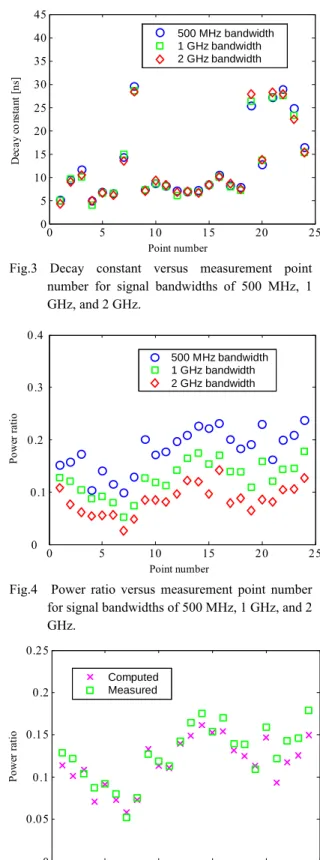
A. Decay Constant

Fig. 3 shows the decay constant of each measured point for signal bandwidths of 500 MHz, 1 GHz and 2 GHz. It seems that the decay constant is slightly dependent on the signal bandwidth with similar results of these three bandwidths at each point. This result is consistent with our analytical result as shown in (3). The mean decay constants of cases 1-4 are 7ns, 12ns, 8ns and 22ns, respectively. It reveals that the mean decay constant tends to increase with the propagation distance. This is because that as the propagation distance is increased, the ratio of the propagation distance of each subsequent MPCs to that of the direct path is decreased, and it leads to larger power gains for delay taps.

B. Power Ratio

Fig. 4 shows the power ratio of each measurement point for signal bandwidths of 500 MHz, 1 GHz and 2 GHz. It is found that the power ratio is decreased when the signal bandwidth is increased, which validates our analytical result as shown in (4). Fig. 5 shows the measured and computed power ratio of each measurement point for 1 GHz bandwidth. Here, the computed results are based on the measured results of a 500MHz-bandwdith signal and using (5). The comparison shows that our proposed method yields good prediction accuracy of power ratio with E (500 MHz, 1 GHz) = 0.0704. Here,_r

(

f1, f2

)

E_r , represents the mean of the relative

prediction error (the ratio of the difference between the predicted and the measured data to the measured data) of power ratio and is given by

( , ) 1

(

( , , ) (, )

)

( , ) 1 1 2 2 2 2 1 = ∑ − = N j p m m r r j f f r j f r j f N f f E (9)

where rp(j, f1, f2) is the computed power ratio of

the jth _{measurement point for bandwidth f} 2 and it

is predicted from the measured results of a signal with bandwidth f1. rm(j, f2) are the measured

power ratio of jth _{measurement point for}

bandwidth f2. For conciseness, the computed

results of power ratio for bandwidths (1 GHz, 2 GHz) and (500 MHz, 2 GHz) with Er(1 GHz, 2

GHz) = 0.1129 and Er(500 MHz, 2 GHz) =

0.1635, respectively, are not illustrated. C. Nakagami Parameter

From our measurement evidence, it is found that the Nakagami parameters, except the first tap, are all closed to 1 (Rayleigh distribution). Therefore, we only focus on the Nakagami parameter of the first tap in this paper. Fig. 6

shows the Nakagami parameter for all the 24 measurement points for signal bandwidths of 500 MHz, 1 GHz and 2 GHz. It is found that the Nakagami parameter is increased when the signal bandwidth is increased, which validates our analytical result. Fig. 7 shows the measured and computed Nakagami parameter of each measurement point for 1 GHz bandwidth. Here, the computed results are based on the measured results of a 500MHz-bandwdith signal. The comparison shows that our proposed method yields good prediction accuracy of Nakagami parameter.

To quantify the prediction accuracy of the Nakagami parameter, the mean of the relative prediction error of Nakagami parameter,

(

f1, f2

)

E_m , is defined and given by

( , ) 1

(

(, , ) (, )

)

(, ) 1 1 2 2 2 2 1 = ∑ − = N j m m p m m j f f m j f m j f N f f E (10)

where mp(j, f1, f2) is the computed Nakagami

parameter of the jth _{measurement point for}

bandwidth f2 and it is predicted from the

measured results of a signal with bandwidth f1.

mm(j, f2) are the measured Nakagami parameter

of jth _{measurement point for bandwidth f}

2. After

some computations, Em

(

f1, f2

)

are equal to

0.3690, 0.1507 and 0.2412 for (f1, f2) equal to

(500 MHz, 1 GHz), (1 GHz, 2 GHz) and (500 MHz, 2 GHz), respectively.

VI. Conclusions

In this paper, the formulas describing bandwidth dependency of UWB channel parameters, such as power ratio, decay constant and Nakagami parameter, are derived under the STDL model. These formulas have been validated by comparing the computed results with a large number of measurement data carried out at laboratories, offices and classrooms with frequencies ranged from 3 GHz to 5 GHz and signal bandwidths of 500 MHz, 1 GHz and 2 GHz. Through these formulas, the values of UWB channel parameters for wide bandwidth signals can be determined from those of narrow bandwidth signals.

In the future, we plan to investigate the bandwidth dependency of channel parameters of S-V model. It is a well-recognized model to characterize the multipath- clustering phenomenon that may be observed in UWB indoor radio channels especially when the signal bandwidth is extended to several GHz.

References

[1] Porcino and W. Hirt, “Ultra-Wideband Radio Technology: Potential and Challenges Ahead,” IEEE Communications Magazine, vol.41, issue 7, July 2003, pp.66-74.

[2] FCC “Revision of Part 15 of the Commission’s Rules Regarding Ultra-Wideband Transmission Systems,” First Report and Order, ET Docket 98-153, FCC 02-48, Apr. 2002.

[3] Dajana Cassioli, Moe Z. Win, Andreas F. Molisch, “The Ultra-Wide Bandwidth Indoor Channel: From Statistical Model to Simulations,” IEEE Journal on Selected Areas in Communications, vol. 20, no.6, Aug. 2002, pp. 1247-1257.

[4] J. D. Parsons, “The Mobile Radio Propagation Channel,” Pentech Press Publishers, London, 1992.

[5] M. Nakagami, “The m distribution; a general formula of intensity distribution of rapid fading,” Statistical Methods in Radio Wave Propagation, W.G. Hoffman, ed., pp. 3-36, 1960

Fig. 1 The averaged power delay profile of a 500MHz- bandwidth UWB signal, which is measured in an indoor environment under NLOS condition.

Fig. 2 Layouts of four measurement sites. (a) laboratory 901; (b) classroom 203, (c) computer room 713; (c) classrooms 301-303.

Fig.3 Decay constant versus measurement point number for signal bandwidths of 500 MHz, 1 GHz, and 2 GHz.

Fig.4 Power ratio versus measurement point number for signal bandwidths of 500 MHz, 1 GHz, and 2 GHz.

Fig.5 Comparisons between the measured and computed results of the power ratio for all of the 24 measurement points at 1 GHz bandwidth

Power ratio r Exponentially power decay constant ε Power ratio r Exponentially power decay constant ε 901 1 2 3 Tx 713 Tx 9 11 12 10 303 302 301 13 14 15 16 17 18 19 20 21 22 23 24 (a) (b) (c) (d) 203 4 6 7 8 5 8×8 measurement grid 3.75 cm 8×8 3.75 cm Tx Tx 901 1 2 3 Tx 713 Tx 9 11 12 10 303 302 301 13 14 15 16 17 18 19 20 21 22 23 24 (a) (b) (c) (d) 203 4 6 7 8 5 203 4 6 7 8 5 8×8 measurement grid 3.75 cm 8×8 3.75 cm Tx Tx 0 5 10 15 20 25 0 5 10 15 20 25 30 35 40 45 500 MHz bandwidth 1 GHz bandwidth 2 GHz bandwidth Point number De ca y c o ns ta nt [ ns] 0 5 10 15 20 25 0 5 10 15 20 25 30 35 40 45 500 MHz bandwidth 1 GHz bandwidth 2 GHz bandwidth Point number De ca y c o ns ta nt [ ns] 0 5 10 15 20 25 0 0.1 0.2 0.3 0.4 500 MHz bandwidth 1 GHz bandwidth 2 GHz bandwidth Point number Po we r r atio 0 5 10 15 20 25 0 0.1 0.2 0.3 0.4 500 MHz bandwidth 1 GHz bandwidth 2 GHz bandwidth Point number Po we r r atio 0 5 10 15 20 25 0 0.05 0.1 0.15 0.2 0.25 Computed Measured Point number Po we r r at io 0 5 10 15 20 25 0 0.05 0.1 0.15 0.2 0.25 Computed Measured Point number Po we r r at io

Fig. 6 Nakagami parameter versus measurement point number for signal bandwidths of 500 MHz, 1 GHz, and 2 GHz.

Fig.7 Comparisons between the measured and computed results of the Nakagami parameter for all of the 24 measurement points at 1 GHz bandwidth. Point number Na ka ga m i pa ra m ete r Point number Na ka ga m i pa ra m ete r Point number Na ka ga mi pa ra me te r Point number Na ka ga mi pa ra me te r