蛋白質二級結構的規則性及其應用

國

立

交

通

大

學

資訊工程系

博

士

論

文

蛋白質二級結構的規則性及其應用

Finding Protein Secondary Structure Regularity

and Related Applications

研 究 生：朱彥煒

指導教授：孫春在 教授

楊進木 教授

蛋白質二級結構的規則性及其應用

Finding Protein Secondary Structure Regularity

and Related Applications

研 究 生：朱彥煒 Student：Yen-Wei Chu

指導教授：孫春在 教授 Advisor：Prof. Chuen-Tsai Sun

楊進木 教授 Prof. Jinn-Moon Yang

國 立 交 通 大 學

資 訊 工 程 系

博 士 論 文

A Dissertation Submitted to

Department of Computer Science

College of Electrical Engineering and Computer Science National Chiao Tung University

in partial Fulfillment of the Requirements for the Degree of

Doctor of Philosophy in

Computer Science

June 2006

Hsinchu, Taiwan, Republic of China

蛋白質二級結構的規則性及其應用

學生：朱彥煒

指導教授：孫春在教授

楊進木教授

國立交通大學資訊工程學系

摘

要

本論文從序列的觀點，討論蛋白質二級結構的規則性。我們定義一個

模式以表示蛋白質二級結構的規則性，並提出一個分群-穩態基因演算法

來找尋符合蛋白質二級結構規則性的模式。在方法的驗證上，針對所提

的演算法利用消去研究法則，証明加入分群的概念是有效果的；並與資

料探勘上常用的關聯規則和決策樹等方法做比較，本方法的確在蛋白質

資料集中，有相對優異的表現。在應用上，我們分析

PSIPRED 和 PROF

這二種方法在做蛋白質二級結構的預測時，有某些區域都是無法猜對

的，但利用我們所提出來的模式，可改進此區域約

40% 至 60% 左右的

預測正確率。進一步，我們將所找到的二級結構模式結合

PSIPRED 和

PROF 的預測結果，可改進目前二級結構的預測。此外，我們亦以此實

驗提出一個教案，以符合問題導向式的學習在生物資訊課程上的教學。

Finding Protein Secondary Structure Regularity and

Related Applications

Student：Yen-Wei Wu Advisors：Dr. Chuen-Tsai Sun

Dr. Jinn-Moon Yang

Department of Computer Science

National Chiao Tung University

ABSTRACT

The author explores protein secondary structure regularity from the

perspective of sequences. Regularity is defined in terms of a schema

discovered by a cluster-based genetic algorithm. Two steps taken to validate

the algorithm were a) finding the weightiness of cluster and b) comparing

the approach with data mining methods. Schemata were used to address

secondary structure predictions for residues that PSIPRED and PROF could

not predict. The results indicate that the proposed schemata can improve

prediction accuracy for these residues by approximately 40% and 60% for

the CB513 and RS126 data sets, respectively.

Furthermore, schemata

combine the prediction results of PSIPRED and PROF to improve secondary

structure prediction. A bioinformatics teaching plan using a problem-based

approach is discussed.

Acknowledgements

I am indebted to several mentors, especially my advisor, Dr. Chuen-Tsai Sun, who showed concern and support for my efforts. He taught me both the proper approach to and attitude toward problem solving. Professor Jinn-Moon Yang taught me the importance of completeness in a study, professor Yuh-Jyh Hu helped me overcome research bottlenecks many times, and professor Jenn-Kang Hwang gave me many valuable suggestions.

I also wish to thank several classmates. Chin-Sheng Yu kindly provided advice on biological principles and bioinformatics tools; we met frequently via MSN whenever I came to a dead end. Ching-Yao Wang gave me many useful suggestions regarding methods. Dai-Yi Wang, Hsu-Chih Wu, and other fellow lab members also assisted me in developing this research.

Finally, this dissertation could not have been completed without the endless love and support from my father, mother, and the rest of my family. I owe all of my achievements to them and send them my love and gratitude.

Contents

ABSTRACT (in Chinese)... i

ABSTRACT (in English) ...ii

Acknowledgements ...iii Contents... iv List of Tables...viii List of Figures... x Chapter 1. Introduction... 1 1.1 Motivation... 1 1.2 Study Importance ... 2 1.3 Thesis Organization ... 3

2.1 Data Sets ... 5

2.2 Clustering (K-means) ... 6

2.3 Genetic Algorithms ... 8

2.3.1 Initializing the Population ... 9

2.3.2 Fitness Function ... 10

2.3.3 Selection... 10

2.3.4 Crossover... 11

2.3.5 Mutation ... 12

2.4 Protein Secondary Structures... 13

2.4.1 Classification... 15

2.4.2 Prediction ... 16

2.4.3 Evaluation ... 19

Chapter 3. Materials and Methods... 23

3.1 Process data set ... 23

3.1.1 PDB_select Constraints... 24

3.1.2 Constraints... 25

3.1.4 Making Training Sets... 29

3.2 Schema ... 30

3.3 Cluster-based Genetic Algorithm... 32

3.3.1 Population and Evaluation ... 36

3.3.2 Steady-state Reproduction ... 38

3.4 Compare with Associate Rule ... 39

3.5 Experimental Results... 43

Chapter 4. Predictive Tools for Protein Secondary Structure ... 46

4.1 EVA ... 47

4.2 PSIPRED and PROF ... 48

4.3 Experiment and Results ... 51

Chapter 5. A Teaching Plan for Bioinformatics... 61

5.1 Introduction... 62

5.1.1 Bioinformatics... 62

5.1.2 Problem-Based Learning... 63

5.1.3 Concept Maps... 64

5.3 A Bioinformatics Teaching Plan... 70

Chapter 6. Conclusions and Future Research... 74

Bibliography ... 77

Appendix A ... 96

List of Tables

TABLE 2.1:DSSP CODES AND THEIR MEANINGS... 15

TABLE 2.2:FIVE CATEGORIES OF MERGE CODES FOR THE THREE DSSP CODES. ... 16

TABLE 2.3:MATRIX FOR NINE PARAMETERS OF EVALUATIVE METHODS. ... 19

TABLE 3.1:STATISTICS FOR 20 AMINO ACIDS IN THE PDB_SELECT CHAIN SET.% IS THE

PERCENT OF EACH AMINO ACID IN THE PDB_SELECT.%H,E% AND L% IS THE

PERCENT OF EACH SECONDARY STRUCTURE RESPECTIVELY IN THE PDB_SELECT... 27

TABLE 3.2:TEST RESULTS OF ARM30,ARM60 AND SSGA(IN NR-PDB) ... 41

TABLE 3.3:TENDENCIES OF VARIOUS AMINO ACID SECONDARY STRUCTURE TYPES... 42

TABLE 3.4:SECONDARY STRUCTURE TENDENCIES FOR EACH AMINO ACID IN NR-PDB

AND PDB_SELECT CHAIN SETS. ... 44

TABLE 4.1:PSIPRED AND PROF PREDICTION ACCURACY PERCENTAGES FOR THE TWO

DATA SETS. ... 53

TABLE 4.2:PERCENTAGES OF EACH PREDICTION CLASSIFICATION FOR THE TWO DATA

SETS... 54

TABLE 5.1:IMPLEMENTATION TABLE FOR PROBLEM-BASED APPROACH TO TEACHING

BIOINFORMATICS... 67

TABLE 5.2:TEACHING PLAN DESIGN USING A PROBLEM-BASED APPROACH FOR

List of Figures

FIGURE 2.1: GENETIC ALGORITHM FLOWCHART. ... 9

FIGURE 2.2:THREE CROSSOVER EXAMPLES. ... 12

FIGURE 2.3:TWO MUTATION EXAMPLES. ... 13

FIGURE 2.4:ILLUSTRATIONS OF ALPHA HELIX AND BETA SHEET... 14

FIGURE 3.1:AN EXAMPLE OF USING SEQUENCE 1CTJ TO MAKE A TRAINING SET. ... 30

FIGURE 3.2:SCHEMA EXAMPLE... 32

FIGURE 3.3:OUR PROPOSED CLUSTERING STRATEGY. ... 34

FIGURE 3.4:OUR CLUSTER-BASED GENETIC ALGORITHM FOR MINING SCHEMATA AND ITS APPLICATION FOR PREDICTING PROTEIN SECONDARY STRUCTURES... 36

FIGURE 3.5:STEADY-STATE STRATEGY FOR OUR CLUSTER-BASED GENETIC ALGORITHM. ... 38

FIGURE 3.6:Q3 ACCURACY IN DIFFERENT CLUSTER NUMBERS USING OUR APPROACH. . 44

FIGURE 4.1:PSIPRED FLOWCHART... 50

FIGURE 4.2:FLOWCHART FOR GENERATING AB,~AB,~A~B,A~B, AND ~AB

CLASSIFICATIONS. ... 52

FIGURE 4.3:SCHEMATA-GENERATING FLOWCHART FOR ADDRESSING DEAD AREAS... 55

FIGURE 4.4:ACCURACY DATA FOR ALL SEQUENCES OF THE DATA SETS AT DIFFERENT

CLUSTER NUMBERS. ... 57

FIGURE 4.5:ACCURACY DATA FOR THE ~A~B CLASSIFICATION OF THE DATA SETS AT

DIFFERENT CLUSTER NUMBERS... 58

FIGURE 4.6:ACCURACY DATA FOR ALL SEQUENCES AND ~A~B CLASSIFICATION FOR

DATA SET RS126... 59

FIGURE 4.7:ACCURACY DATA FOR ALL SEQUENCES AND ~A~B CLASSIFICATION FOR

FIGURE 5.1:IMPLEMENTATION FLOWCHART FOR PROBLEM-BASED APPROACH TO

TEACHING BIOINFORMATICS... 66

FIGURE 5.2:AN EXAMPLE OF A SPIDER-WEB MAP. ... 68

FIGURE 5.3:AN EXAMPLE OF A CHAIN MAP. ... 69

Chapter 1.

Introduction

1.1 Motivation

Protein sequences consist of different combinations of a four-letter DNA alphabet (A, G, C and T) that is used to create a 20-word vocabulary of native amino acids. Genes are considered the blueprint or library of life, and proteins the machinery. Proteins are macromolecules that perform all-important tasks in organisms, including the catalysis of biochemical reactions, nutrient transport, and signal recognition and transmission.

Protein function is determined via a three-dimensional structure [1]. Researchers know that determining protein structure in a laboratory is much more difficult than identifying protein sequence. This explains why as of March 6, 2006 the Protein Information Resource (PIR) database contained 2,826,393 protein sequence records while

Independent researchers and an organization known as the Critical Assessment of Techniques for Protein Structure Prediction (CASP) currently support the practice of predicting protein structure from previously known sequences [4, 5, 6, 7, 8].

Protein secondary structure is very valuable information for predicting 3D protein structure. In many applications (e.g., identifying protein functions, classifying proteins, establishing phylogenetic trees), protein structure knowledge requires information on protein secondary structure. [9, 10, 11]. The present research—analyzing the natural instincts of protein secondary structure and its potential for assisting in protein secondary structure prediction—was motivated by the bottleneck that secondary structure researchers are currently dealing with [12].

1.2 Study Importance

Protein secondary structure is considered crucial to understanding protein tertiary structure [13, 14, 15, 16, 17]. However, even though secondary structure data is often used for protein recognition and protein structure prediction [18, 19, 20, 12, 21, 22], few attempts have been made to determine shared secondary structure patterns. Based on studies describing statistical regularity between single amino acids and various secondary structures [23], some researchers are suggesting that secondary structure formation may (at

least to a certain degree) be determined by sequential amino acid interaction [24]. At the center of this thesis is a proposed representative schema for amino acid interactions as an aid for analyzing their relationship with various protein secondary structures.

One challenge is uncovering schema details—that is, the regularity of protein secondary structures. To avoid predictive deviation in the learning stages of various methods, data sets such as RS126 or CB513 usually have low sequence identity for protein secondary structure. The proposed solution to this problem described in this thesis involves a cluster-based genetic algorithm, since traditional data mining methods (e.g., arm and decision trees) cannot be used with such kinds of data sets.

1.3 Thesis Organization

A review of related studies is presented in Chapter 2. The chapter will also include a discussion concerning the construction of a data set from pdb_select list (except for RS126 or CB513), clustering methods, protein secondary structure prediction, and problem-based learning. Details on the defined schema and the steady-state strategy that was incorporated into the genetic algorithm are presented in Chapter 3, along with an analysis of the proposed cluster-based genetic algorithm. Two applications (predicting protein secondary

and 5, respectively. Conclusions and suggestions for future research will be given in Chapter 6.

Chapter 2.

Related Work

2.1 Data Sets

Rost and Sander (1993) selected 126 proteins for the training and testing of secondary structure prediction algorithms [24]. Their definition of non-redundancy states that no two proteins in a set share more than 25% sequence identity over a length of more than 80 residues. Unfortunately, the RS126 set contains protein pairs that are very similar in terms of sequence according to methods considered more sophisticated than sequence identity percentage. Cuff and Barton’s CB513 dataset [25], consisting of 513 chains with low similarity, has been used to evaluate classifier accuracy. Almost all sequences found in the RS126 set are included in the CB513 set. Both are non-homologous, but CB513 homology

In addition to RS126 and CB513, we established a data set based on the PDB_select protein chain list. The chain list is a representative of PDB chain identifiers that researchers use in order to save considerable time and effort. The PDB_select protein chain list allows for introductory browsing, protein architecture analysis, prediction method development, and model building via modular construction [26].

2.2 Clustering (K-means)

K-means is one of the simplest unsupervised learning algorithms capable of solving the well-known clustering problem [27]. Its main idea is to define one k centroid for each cluster. Care must be taken with centroid placement because different locations will lead to different results. The best approach is to place them as far away from each other as possible. The next step is to take each point belonging to a given data set and forge an association between it and the nearest centroid. When no points are pending, the first step is completed and an early groupage is performed. At this point it is necessary to re-calculate k new centroids as barycenters of clusters produced in the previous step. The

appearance of k new centroids means that more binding must be performed between the same data set points and the new set of nearest centroids. This generates a loop that allows for the step-by-step observation of changes in k centroid locations until no more changes are required (i.e., the centroids stop moving). This algorithm minimizes the chosen distance between a data point and cluster center.

The algorithm consists of four steps:

1. Place K points into the space represented by the objects to be clustered. These points represent initial group centroids.

2. Assign each object to the group containing the closest centroid.

3. After all objects have been assigned, recalculate the K-centroid positions.

4. Repeat steps 2 and 3 until the centroids stop moving. This produces groups for calculating the metric to be minimized.

Although the procedure always terminates at some point, the k-means algorithm does not necessarily find the most optimal configuration that corresponds to a minimum global objective function. The algorithm is also significantly sensitive to the initial cluster centers that are randomly selected—though it can be run multiple times to reduce this effect. For

this reason, the k-means algorithm has been adapted for use with many problem domains [28, 29, 30, 31, 32].

2.3 Genetic Algorithms

Holland’s original genetic algorithms [33] included a well-known heuristic algorithm inspired by Darwin’s theory of evolution (“survival of the fittest”). Later efforts by Goldberg and others have allowed genetic algorithms to be applied to optimization and search problems in many fields [34, 35, 36, 37, 38, 39, 40]. Genetic algorithms do not always find optimal solutions, but in large search spaces they are more efficient than most exhaustive search techniques in attaining near-optimal solutions.

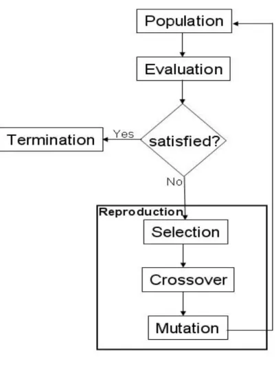
For any given problem, genetic algorithms alternate between working on coding space and solution space [41]. Coding space work involves the need to know how to transfer real problems into chromosomes and to work with chromosomal evolution. These chromosomes are evaluated in the solution space. The major parts of simple genetic algorithm operations are shown in Figure 2.1.

Figure 2. 1: Genetic algorithm flowchart.

2.3.1 Initializing the Population

A population consists of a set number of chromosomes, with each chromosome serving as a candidate solution. A chromosome consists of genes, with each gene serving as a feature of a problem. The feature called genotype in a gene and phenotype in a

problem. At the beginning of the evolutionary process, a binary code or character is randomly assigned to each gene in a chromosome. Through competition among chromosomes in a population, either one or a set of chromosomes eventually satisfies pre-established requirements.

2.3.2 Fitness Function

For a given problem, a specific fitness function must be designed to determine whether a chromosome is a good candidate for survival [42, 43, 44]. In a genetic algorithm, the fitness function plays a guiding role in this determination—in other words, the dual purposes of the fitness function is to consider problem characteristics and to assemble domain knowledge [45, 46, 47, 48].

2.3.3 Selection

Each chromosome has a fitness value (score) that is determined by the fitness function. Chromosomes with higher fitness values are considered more fit for survival, have a higher probability of producing offspring, and tend to dominate other chromosomes in a

population. However, higher scores do not guarantee that a chromosome contains good genes only, nor do low scores indicate a complete lack of genes for positive characteristics. Accordingly, the presence of niche chromosomes must be taken into account when designing a genetic algorithm [49, 50, 51, 52, 53].

2.3.4 Crossover

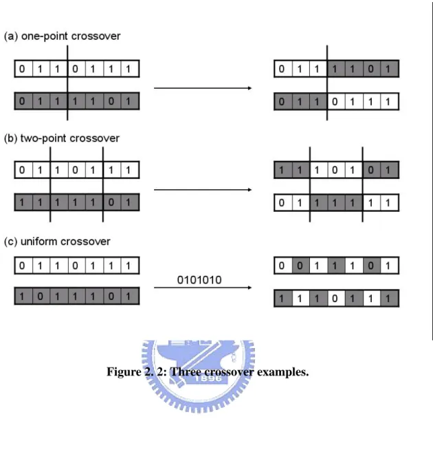
Each pair of chromosomes has what is called a crossover rate—that is, a probability for proceeding crossover. Based on a pre-assigned crossover rate, two chromosomes randomly exchange their genetic information [54, 55]. One-point or two-point crossovers entail cutting and exchanging genes, whereas uniform crossover genes are exchanged according to a random template. Examples of these crossover types (all commonly found in genetic algorithms [56, 57, 58] are shown in Figure 2.2.

Figure 2. 2: Three crossover examples.

2.3.5 Mutation

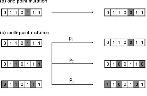
Each chromosome has a mutation probability called a mutation rate. Based on pre-assigned mutation rates, individual genes are randomly chosen to change their value from 0 to 1 or from 1 to 0 (Fig. 2.3a) [59, 60, 61]. An example of multi-point mutation is shown in Figure 2.3b. In that figure, P1, P2, and P3 are three pre-assigned probabilities. P1

is much larger than the others and P2 is bigger than P3. In addition to avoids falling into the local optima area, mutations also maintain chromosome diversity [62, 63].

Figure 2. 3: Two mutation examples.

2.4 Protein Secondary Structures

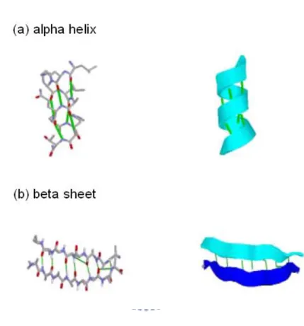
confirmed via x-ray diffraction [66, 67], which describes the chemical structure of a protein based on the primary structure. Later research determined that protein secondary structures express local spatial structure in certain linear segments.

Figure 2. 4: Illustrations of alpha helix and beta sheet.

A randomly generated protein chain may have a loop structure. Achieving a stable conformation requires a large number of weak bonds (e.g., hydrogen bonds, salt bridges and van der waal interactions). Stable conformations are called protein secondary structures. So far, there are 90% residues be located in alpha helix or beta sheet in the database.

2.4.1 Classification

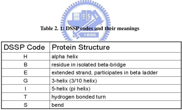
Protein secondary structures have many classifications. The three most common are DSSP, STRIDE, and DEFINE [68, 69, 70]. DSSP (Database of Secondary Structure in Protein), a widely applied classification for protein secondary structure, includes a computer program for defining various features of a protein via a PDB protein structure file. DSSP files include data on secondary structure, molecular properties, and solvent accessibility. Seven DSSP codes for protein secondary structures are shown in Table 2.1.

Table 2. 1: DSSP codes and their meanings

Protein secondary structures are usually predicted using three of the seven DSSP codes: H (helix), E (sheet) and L (loop; this is sometimes referred to as C, coil) [71, 72, 73].

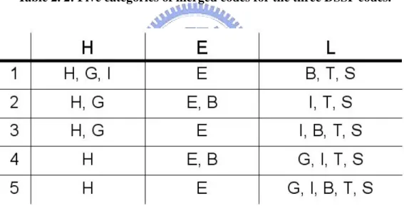
The five categories for the three kinds of DSSP codes are shown in Table 2.2; it is important to note category choice has an important effect on protein secondary structure prediction accuracy [71]. Jones [74] has shown that the fifth category in Table 2.2 performs best for protein secondary structure prediction, but the first category is more commonly used for comparisons with the PHD approach. In 1999, Baldi proposed three new categories: H (H, G, I), E (B, E) and C (T, S) [75].

Table 2. 2: Five categories of merged codes for the three DSSP codes.

2.4.2 Prediction

Most secondary structure prediction methods make use of the fact that segments of consecutive residues have preferences for certain secondary structure states [76, 77]. The

prediction problem is thus transformed into a pattern-classification problem that can be addressed by pattern recognition algorithms, with the guiding goal being to predict whether the residue at the center of a segment of 13-21 adjacent residues has a helix, strand, or no regular secondary structure (loop or coil).

Before the protein secondary structure hypothesis was proven and accepted, biologists tried a variety of approaches to predict protein secondary structure, including the use of protein sequences [78]. All of these methods can now be placed in three categories based on their original assumptions [12]. These categories can also be described in terms of generations.

Secondary structure prediction methods in the first generation focused on four types of residues: helix, sheet, loop former and breaker. Protein secondary structure segments were predicted by considering the characteristics of a single residue [79]. These methods assume that when an amino acid forms a secondary structure, the amino acid acts independently. However, we now know that amino acids are affected by their adjacent amino acids, therefore, accuracy for this method is approximately 50-60%. Method names include Chou & Fasman, GOR1, and Lim [79, 80, 81].

Second generation methods consider local information in residues 3-51, using a fixed window size for a protein sequence and a sliding window for cutting several segments.

Secondary structures are retrieved from these segments. Second-generation method accuracy is only about 60-65% due to a lack of long-distance information—for example, information on the effect of hydrogen bonds between two amino acids separated by a long distance. Method names include GOR3[82], Levin et al. [83], Nishikawe and Ooi [84], Qian and Sejnowski [85], Holley and Karplus [86], Asai et al.[87], and Yi and Lander [88].

Third generation methods added evolution information to the second generation concept [12]—that is, gene mutation occurs as part of the evolutionary process, meaning that one amino acid can be replaced by another. Accordingly, proteins with similar structures may have different amino acids in the same position. Almost all third generation methods take into account multiple sequence alignment results when inputting data into a learning model such as neural networks or SVM. The best-known third generation method, PHD, can reach 70% accuracy or higher for Q3 predictions and over 80% for helix predictions.

Method names include Zvelebil et al. [89], PREDATOR [90, 91], NNSSP [92], DSC [93], PHD [24], Jnet [94], PSIPRED [74], Baldi et al. [75, 95] and HMMSTR [96].

2.4.3 Evaluation

Rost and Sander’s (1993) arrangement of evaluative methods for protein secondary structure prediction is shown as Table 2.3. Its evaluative method parameters have been placed in a 3x3 matrix (for three kinds of secondary structures).

Table 2. 3: Matrix for nine parameters of evaluative methods.

In the matrix, Aij is the number of those residues that belong to secondary structure i

but are predicted for secondary structure j.

To sum up each element in the column, ai, is the predictive number for each

secondary structure.

∑

∑

To sum up all elements in the matrix, b, is the number of residues.

∑

∑

For examples, the secondary structure H has (AHH + AHE + AHC) residues, and there are

(AHH + AEH + ACH) residues predicted to H.

Overall 3-state accuracy, Q3, is a score for secondary structure prediction [97, 85, 12, 88, 98, 99]. It is the most popular evaluative method and shown as follows,

100 3 x b A Q i ii

∑

On the other hand, we can simply discuss the evaluation for each secondary structure. There are two kinds of evaluative methods for predictive accuracy discussed. One show the predictive accuracy of secondary structure i,

100 x b A Q Q i ii obs i i = = , for i = H, E, C

The other show the percentage that how many residues are predicted correctly in the predictive number of secondary structure i.

100 x a A Q i i ii pre i

∑

Matthew’s correlation coefficient, C, is also usually discussed when measure the accuracy of secondary structure shown as follows [100].

) )( )( )( ( i i i i i i i i i i i i i o n u n o p u p o u n p C + + + + − = , for i = H, E, C

pi is those who residues are belong to secondary structure i, and the predictive result is

also i.

ii i A

p = , for i = H, E, C

ni is those who residues are not belong to secondary structure i, and the predictive

∑ ∑

ui is those who residues are belong to secondary structure i, and the do not be

predicted to i.

∑

oi is those who residues are not belong to secondary structure i, but the predictive

result is i.

∑

Chapter 3.

Materials and Methods

3.1 Process data set

We established a data set according to the PDB_select protein chain list because it is representative of PDB chain identifiers that help researchers save considerable time and effort. The PDB_select protein chain list allows for introductory browsing, protein architecture analysis, prediction method development, and model building via modular construction [26].

3.1.1 PDB_select Constraints

There are many versions, from which no two proteins have more than 25% sequence identity to 95%, in the PDB_select list. Furthermore, it excludes chains according to the following criteria:

‧ length less than 30 residues;

‧ number of non-standard amino acid residues (including chain breaks) exceeds 5 percent of chain length;

‧ resolution exceeds 3.5 angstroms;

‧ R-factor exceeds 30 percent;

‧ some chains are known to be of inferior quality;

‧ number of residues without side chain coordinates < 90 percent chain length;

‧ number of residues without backbone coordinates < 90 percent chain length;

‧ content of ALA plus GLY exceeds 40 percent of chain length; and

3.1.2 Constraints

We separated the data set into two independent sets (training and testing) and used the most stringent 25% PDB_select list (2,485 chains with 388,067 residues). Next, we located the secondary structures of proteins in the 25% PDB_select list from the Database of Secondary Structure in Proteins (DSSP) of secondary structure assignments for all PDB protein entries. However, due to problems with DSSP secondary structure information, we eliminated some chains from the 25% list for the following reasons:

‧ incorrect PDB identification in the 25% list;

‧ no information in the DSSP files;

‧ broken chains; or

‧ inclusion of an unknown symbol X.

Our data set consisted of 1,600 chains with 248,984 residues. We randomly selected 1,200 chains for use as a training set for mining schemata; the remainders were used for testing.

3.1.3 Data Set Analysis

It was assumed that the distribution characteristics of the data set would affect the experimental results. We used the data in Table 3.1 to inspect a) whether a relationship exists between the amount of a schemata and the percentage of each amino acid in the data set, and b) the individual tendencies of all amino acids in the data set. Data in the first column of Table 3.1 are for 20 amino acids and second and third column data represent the number of occurrences for each amino acid and their respective percentages. The final column contains data on the corresponding amino acids, number of occurrences, and percentage of secondary helix (H), sheet (E), and Coil (L) structures. The first row presents information on the number of occurrences and percentages of each secondary structure in the data set.

Table 3. 1: Statistics for 20 amino acids in the PDB_select chain set. % is the percent of each amino acid in the PDB_select. %H, E% and L% is the percent of each secondary structure respectively in the PDB_select

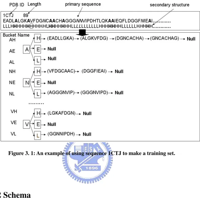
3.1.4 Making Training Sets

For every protein sequence, each amino acid can be viewed as a central amino acid in a schema. We defined amino acids on both sides of a central amino acid as a “neighbor pattern.” According to our size choice of 9 windows, neighbor pattern length = 8, or 4 amino acids on each side. To create the training set we placed the neighbor pattern into a corresponding bucket according to the central amino acid and secondary structure; a partially assigned training set is shown in Figure 3.1. A complete training set consists of 20*3 buckets. Using the fifth amino acid in the 1CTJA protein sequence as an example, the neighbor pattern EADLLGKA should be put into bucket AH, since the central amino acid is A and its secondary structure is H.

Figure 3. 1: An example of using sequence 1CTJ to make a training set.

3.2 Schema

Protein secondary structures are designated as H (alpha helix, 3/10 helix, pi helix), E (beta bridge, beta ladder), or L (turn, bend) [76]. The regularity of secondary structures (which consist of amino acids and one secondary structure) are usually discussed in terms of factors that cause amino acids to combine in order to form a specific secondary structure. An amino acid that plays a role in certain secondary structures are affected by neighboring amino acids, while secondary structure sheets often require extra consideration for remote

amino acids. In the same manner that many researchers de-emphasize the effect of remote amino acids on protein secondary structure [88], we decided to underplay the remote effect in order to simplify schema design.

Representation

We modified Holland’s (1975) one-dimensional schema format

schema s∈{1, 0, *}l

(where l is a fixed length and * is either 0 or 1) into a two-dimensional format:

schema s∈{an amino acid, *} (l-1)/2 X {an amino acid} X {an amino acid, *} (l-1)/2 　

→ {H, E, L| one kind of secondary structures},

where l is a fixed length (an odd number) and * is don’t care.

According to our proposed schema, the central amino acid plays a role that corresponds to a specific secondary structure due to non-asterisk amino acids on each of its two sides. In Figure 3.2, amino acid A is found in the first and last positions and amino acid L is in the center position. Amino acid L is eventually categorized as having an H protein secondary structure—in other words, L is only affected by the first position amino acid on its left side and fourth position amino acid on its right. The other asterisk positions (which have no affect on L) can consist of any amino acid. We focused on the 9 windows in the front part of the schema, since that length is long enough to contain sufficient local structural information for analysis [101].

Figure 3. 2: Schema example.

3.3 Cluster-based Genetic Algorithm

Average Q3 accuracy in studies of protein secondary structure prediction using genetic algorithms is only 46 percent. Three issues are considered central to this problem: data set selection, solution search space, and fitness function design. At first, for the data

set in previous studies, RS130 cannot represent so far the whole known proteins. Moreover, the number of similarities among DSSP protein families is considered too high. These kinds of problems are not associated with PDB_select.

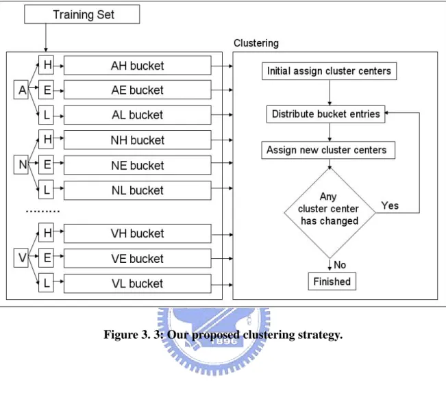
Based on the 9-window size of the schema we applied, search space size is 20*3*21*8. To reduce search time, the very important thing is let genetic algorithm can search from good start. Therefore, once clustering was completed, we placed cluster centers as chromosomes into the initial population (Fig. 3.3).

Figure 3. 3: Our proposed clustering strategy.

The fitness function gives evolutionary direction to chromosomes [102]. When designing our fitness function, we assumed that a good schema should have a strong tendency toward a certain secondary structure. Furthermore, our fitness function states that increased chromosome confidence in the training set also increases Q3 accuracy in the protein secondary structure prediction.

As shown in Figure 3.4, our model includes evolutionary and application phases. With the exception of standard GA steps, during the evolutionary phase we generated some

initial chromosomes by clustering. The evolutionary process makes use of a steady-state strategy. In each generation we placed certain high fitness chromosomes into our schemata set. Chromosomes placed in the set were removed from the population; the population consequently generated new chromosomes at random.

For protein secondary structure predictions we cut the sliding windows (9 window lengths) to use as protein sequence patterns for testing. Each pattern aligns with all schemata in the schemata set. After alignment, the secondary structure of the most similar schema was selected as the predictive result. When the fitness of the most similar schema was insufficient, the pattern was aligned with the neighbor patterns of cluster centers in the training set. The final predictive result was the secondary structure that the most similar cluster center belonged to. Our approach uses blosum62 as a substitution matrix for alignment purposes.

Figure 3. 4: Our cluster-based genetic algorithm for mining schemata and its application for predicting protein secondary structures.

3.3.1 Population and Evaluation

Our approach uses 20 populations for each amino acid. Each chromosome includes a neighbor pattern and a secondary structure. Initial populations take on the neighbor pattern of the cluster center; all other chromosomes are randomly generated.

To evaluate a chromosome, we used its neighbor pattern for alignment with neighbor patterns in all secondary structure buckets. Alignment scores that exceeded a certain

threshold were labeled as one hit. nH, nE, and nL are the respective hit numbers in the H, E, and L buckets. Chromosome secondary structure is determined according to the maximum hit number.

In the following equation,

confidence=nSS/(nH+nE+nL) (1),

nSS is defined as the maximum hit number among nH, nE, and nL. Confidence is

relative to Q3; one of our goals was to find schemata with distinct tendencies toward certain secondary structures. We defined the discrimination rate (DR) as

DR=(nHighest-nSecond)/(nH+nE+nL) (2),

where nHighest is equal to nSS and nSecond is the second highest score among nH,

nE, and nL. As a result,

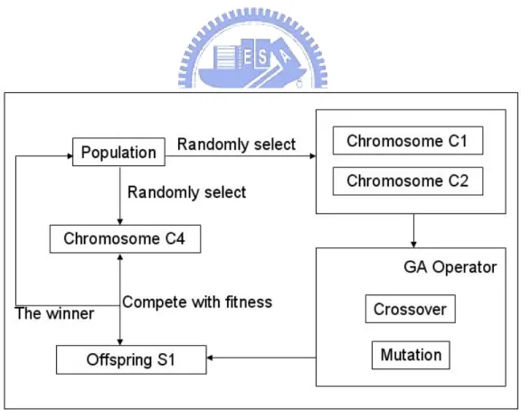
3.3.2 Steady-state Reproduction

The initial step in the steady-state strategy shown in Figure 3.5 is to randomly select two chromosomes, C1 and C2. Two offspring are generated by one-point crossover and multi-point mutations of C1 and C2; a single S1 offspring is randomly selected from these two offspring. Another chromosome (C4) is selected from the population for comparison with the S1 offspring in terms of fitness. The best chromosome is used to replace C4 in the population.

3.4 Compare with Associate Rule

The training set consists of 124 protein sequences each of which has more than 80 amino acids in length, and the pairwise similarity is below 25% (similar to RS130 [24]). They were used to train SSGA to find significant schemas associated with various protein secondary structures. To obtain the confidence and support value, we tested SSGA on the nr-PDB data set created by NCBI after removing those sequences used for training. If A ⇒

B is the form of rules, and P(A ∪ B) is a probability of both A and B. The confidence and

support value are defined as

matches schema of number tions classifica correct of number A) | P(B B) (A confidence ⇒ = = (4) matches structure secondary of number tions classifica correct of number B) P(A B) (A support ⇒ = ∪ = (5)

To reduce time complexity, we adopt FP-growth algorithm for association rule mining to avoid generating candidates from the frequent itemsets [103]. Before using the ARM method for schema finding, we need to set two criteria (confidence and support). In our training set, 124 protein sequences could be further sampled into 23,448 transactions (obtained through sliding window sampling within the protein sequence, window size=9). The support value in the worst case is 4.264e-5 (1/23448). In order to discover more possible patterns, the support value could be set as 5e-5 in this experiment

A higher confidence value schema means it has a higher relationship between sequence and structure (like the form shown in figure 3.2) within the training data. Thus we assume that such schema could have higher confidence in testing data. The result of this assumption will be explained in the subsequent experiment. We run ARM with two different confidence values. The confidence value of ARM30 is 30% and ARM60 is 60% in the training set. Table 3.2 illustrates the performance of ARM30 and ARM60 under the testing set (nr-PDB). All 11 schemas of ARM30 fall within the bracket (0%-10%). However, ARM60 has a higher and broader confidence range (20%-50%).

Table 3. 2: Test Results of ARM30, ARM60 and SSGA (in nr-PDB)

After the evolutionary process terminated, we checked each of the twenty converged populations to get the most frequent secondary structures for every amino acid. We summarize the results in Table 3.3. It shows that most of the natural correlations between amino acids (statistics from nr-PDB) and the preferred structures were also found in the converged populations (evolved by SSGA) with one exception of amino acid Y. Note that all the initial populations were randomly generated. The finding of similar correlations between amino acid preferences toward particular structures in the final converged populations certainly provides some confidence of the fitness function applied in SSGA.

Table 3. 3: Tendencies of various amino acid secondary structure types

The learned schemas from the training set were later tested on the nr-PDB test set to measure their confidence and support values. Finally, there are 904 total possible rules to be found. The average confidence value is 61.51% and nearly half of mined rules are over 70%. Table 3.2 is the testing results of ARM30, ARM60 and the SSGA approach. It could be divided into three parts, the left-hand column shows the total mined schema number from compared methods; the central part shows the number of schemas mined from different confidence ranges (10% increments); and the right-hand part shows the aver-age of confidence and support value. Hence, table 3.3 clearly shows that the average value of confidence and support from the SSGA approach are significantly higher than the ARM method.

If the average support value of the significant schemas is 1%, then we need approximately 9861 (986059*1%) significant schemas to handle all known proteins. So the number of schemas are not enough to predict secondary structure in our results.

3.5 Experimental Results

3.5.1 Clustering-based SSGA

Since our approach uses a clustering strategy for the initial population, we ran several trials using cluster numbers between 20 and 70 to predict protein secondary structures; results are shown in Figure 3.6.

At 70 clusters our Q3 accuracy was 58.7 percent—approximately 12 percent better than predictive results from studies using genetic algorithms only.

Figure 3. 6: Q3 accuracy in different cluster numbers using our approach.

3.5.2 Illustrate Some Interesting Schemata

Table 3.4 presents a comparison of our Table 3.1 results with nr-PDB. Several differences are observed when K, W, and Y are in both PDB_select and nr-PDB. This underscores the importance of selecting a suitable data set.

Table 3. 4: Secondary structure tendencies for each amino acid in nr-PDB and PDB_select chain sets.

Selected schemata with interesting biological meaning and high fitness are displayed in Table3. The central amino acid in the first schema is P; when its neighbor pattern is D***P**N, the central amino acid plays an L role in the secondary structure. Note that L is the tendency for D, P, and N in Table 3.5.

Chapter 4.

Predictive Tools for Protein

Secondary Structure

Even though the protein folding process may require catalysts [104], it is widely accepted that the three-dimensional structure of a protein is associated with its amino acid sequence [105]. This implies the possibility of predicting protein structure from a sequence. However, with the increasing number of amino acid sequences generated by large-scale sequencing projects and the continuing shortage of data on crystallized homologous structure, the need for reliable structural prediction methods is greater than ever.

Making accurate comparative assessments of different secondary structure prediction methods is difficult because they use different learning process datasets and different secondary assignments [106]. Still, a number of authors have designed methods

with accuracies above the 70% threshold by taking advantage of multiple sequence alignments [24, 92, 93, 107, 108] or selected alignment fragment pairs [91]. Most methods do not take the long-distance (beta sheet) effect into consideration because it is difficult to incorporate this feature into a model. Accordingly, secondary structure prediction accuracy appears to have reached its current limits. Analyses of several predictive tools indicate that approximately 12% of data set residues (dead areas) cannot be predicted. The complete schemata for all proteins have not yet to be identified because of a need for additional protein information. However, tests indicate that the schemata described in this paper can improve dead area prediction accuracy by 40% to 60%.

4.1 EVA

EVA (EValuation of Automatic protein structure prediction) is a plan for evaluating protein structure predictive tools [109]. Its users can evaluate tools associated with secondary structure, comparative modeling, and threading. EVA constantly downloads the latest protein structure data from PDB. Structures are added to mySQL databases; after sequences are extracted for each protein chain, they are sent to prediction servers via META-PredictProtein (META-PP), which collects the results and sends them to EVA. Each week EVA runs alignment programs for sequence searches and structure

databases to determine homologues. Secondary structure predictions, inter-residue contact predictions, and comparative modeling are evaluated by personnel at EVA satellites (Columbia University, Rockefeller University, and CNB Madrid). Employees at the central EVA site at Columbia University collect all assessments from the other two centers as well as results from database searches, then publishes the information on its main web site. Mirror web sites are maintained at the other EVA satellite locations.

EVA has evaluated at least 10 types of secondary structure predictive methods. Two of these methods, PSIPRED and PROF, were selected for this experiment, based on their proven predictive abilities and their accessibility in terms of downloads.

4.2 PSIPRED and PROF

A two-stage neural network has been used to predict protein secondary structure based on position-specific scoring matrices generated by PSI-BLAST. This approach, proposed by Jones in 1999, is called PSIPRED. PSIPRED used a new test set based on 187 unique folds and three-way cross-validation based on structural similarity criteria rather than previously favored sequence similarity criteria. Its predictive accuracy achieved an average Q3 of 76.5% to 78.3%, depending on the definition of observed secondary structure.

The three stages of this prediction method are generating a sequence profile, predicting an initial secondary structure, and filtering the predicted structure (Fig. 4.1). The dual goals are to generate sequence profiles and to predict secondary structure. Standard approaches to generating sequence profiles are considered cumbersome and time-consuming. The PSI-BLAST method uses profiles as direct input to secondary structure prediction rather than extracting sequences and creating an explicit multiple sequence alignment as a separate step. The time-consuming multiple sequence alignment task is eliminated by using PSI-BLAST profiles directly. The final position-specific scoring matrix from PSI-BLAST is used as neural network input. The matrix has 20 x M elements, with M representing the target sequence length and each element representing the log-likelihood of a particular residue substitution at a template position based on a weighted average of BLOSUM62 matrix scores for the given alignment position.

Figure 4. 1: PSIPRED flowchart.

PSIPRED utilizes a standard feed-forward back-propagation network architecture [110] with a single hidden layer. A window of 15 amino acid residues (producing an overall Q3 score of 80.1%) is considered optimal, therefore the final input layer consists of 315 input units divided into 15 groups of 21 units each. A large hidden layer of 75 units was used, with another three units (representing the three states of secondary structure—helix, strand or coil) being used to create the output layer. As with previous neural network secondary structure prediction methods [24], a second network is used to

filter successive outputs from the main network. Since only three inputs are necessary for each amino acid position, this network has an input layer of only 60 units divided into 15 groups of equal size. In this project, a smaller hidden layer of 60 units was used for this network.

PROF is a method proposed by Rost [111]. However, the author has created a downloadable version for predicting secondary structures. PROF is described as an improved version of PHDsec—a profile-based neural network predictor of protein secondary structure.

4.3 Experiment and Results

The two purposes of this experiment were to locate the shared bottleneck of the three generation methods in predicting protein secondary structures—in other words, determining if some residues exist that neither PSIPRED nor PROF can predict. The region that contains these residues, known as the “dead area,” is shown in Figure 4.2. The second purpose was to activate the dead area by inserting the proposed schemata.

Figure 4. 2: Flowchart for generating AB, ~AB, ~A~B, A~B, and ~AB classifications.

PSIPRED and PROF predictive results are shown in Table 4.1. The results were used to define the following symbols:

A: successful PSIPRED prediction area,

~A: failed PSIPRED prediction area,

B: successful PROF prediction area,

~B: failed PROF prediction area.

PSIPRED and PROF predictive results were observed simultaneously and divided according to five classifications:

AB: areas where PSIPRED and PROF produced the same successful prediction,

~(AB): areas where PSIPRED and PROF produced the same failed prediction,

~A~B: areas where PSIPRED and PROF produced different predictions, both of them failed,

A~B: areas that PSIPRED predicted successfully but PROF did not, and

~AB: areas that PROF predicted successfully but PSIPRED did not.

Table 4. 1: PSIPRED and PROF prediction accuracy percentages for the two data sets.

The percentages of these five classifications for data sets RS126 and CB513 are shown in Table 4.2. The data indicate type AB percentages that exceed 70% for both sets, meaning that third-generation secondary structure predictive methods that include evolution information can improve accuracy to 70%. The percentage of the type A~B classification

the two methods made an identical but incorrect prediction—type ~(AB)—less than 1% of the time, indicating a 98% prediction confidence when the same result was predicted by both methods. The last type (~A~B) represents the dead area, which neither was able to predict, but with different results; coverage for this area was 12%. Accordingly, the upper boundary for secondary structure prediction accuracy for third generation methods is approximately 88%.

Table 4. 2: Percentages of each prediction classification for the two data sets.

The proposed schemata were applied to dead areas for the purpose of improving secondary structure predictions. A schemata experiment flowchart is shown in Figure 4.3. In the first part of the experiment, predictions were generated by PSIPRED and PROF for the RS126 and CB513 data sets. The two predictive results were compared for the purpose of defining the dead area. The second part of the experiment focused on using the proposed cluster-based genetic algorithm to derive schemata from PDB_select. Each case was run

several times using different cluster numbers to predict RS126 and CB513 secondary structures.

Figure 4. 3: Schemata-generating flowchart for addressing dead areas.

Although the predictive ability of the proposed schemata did not surpass that of the third-generation prediction methods, it did produce balanced predictive results according to the five classifications described above. It is therefore suggested that the proposed schemata can be used to assist PSIPRED and PROF in predicting secondary structures in dead areas. We observe the accuracy of all data set and dead area only in the different

parameter value of cluster number. Predictive accuracies for all RS126 and CB513 sequences produced by the proposed schemata are shown in Figure 4.4. The highest prediction accuracy figures for RS126 (73%) and CB513 (60%) were achieved when cluster number equaled 70. PSIPRED and PROF were capable of 80.9% and 80.5% accuracy for RS126 and CB513, respectively, but neither method was capable of correctly predicting any residues in dead areas—in other words, their predictive accuracy for dead areas was 0%. Dead area prediction accuracies using the proposed schemata were 58% for RS126 when the cluster number was 70 and 38% for CB513 when the cluster number was 60 (Fig. 4.5). Figure 4.6 presents data for when the proposed schemata were used to predict all sequences and dead areas in RS126. As shown, in each case accuracy increased. However, for CB513 the dead area prediction accuracy increased slowly as the predictive accuracy for all sequences increased (Fig. 4.7).

Figure 4. 4: Accuracy data for all sequences of the data sets at different cluster numbers.

Figure 4. 5: Accuracy data for the ~A~B classification of the data sets at different cluster numbers.

Figure 4. 6: Accuracy data for all sequences and ~A~B classification for data set RS126.

Figure 4. 7: Accuracy data for all sequences and ~A~B classification for data set CB513.

Chapter 5.

A Teaching Plan for Bioinformatics

Bioinformatics research requires input from several different domains, but the majority of bioinformatics learners are unfamiliar with specific biological issues. We propose an approach that combines problem-based learning and concept map methodology to realize and construct the biological problems. As part of the problem-solving process, learners must gather materials and identify essential knowledge—thus creating a scenario conducive to learner training. We believe this approach will be of great use to non-biologist learners in the bioinformatics field.

The human genome project has attracted a large number of information science researchers to work in the area of bioinformatics. Of particular interest to these researchers

large bodies of data. However, information science experts have little understanding of biology, and only a handful of biologists understand information algorithm requirements.

In this section, we will propose a problem-based learning approach that makes use of concept maps for bioinformatics learning. Our goals are to a) create a process through which information specialists can easily identify the core issues of biology problems, and b) reduce research costs associated with applying information theory to biology problems.

5.1 Introduction

5.1.1 Bioinformatics

In 1989, the U.S. National Institutes of Health invited James D. Watson—best known for describing the double-helix structure of DNA—to establish a human genome research center. The guiding objective for researchers from the United States and 17 other countries has been to identify over 3 billion DNA sequences that make up the human genetic code. The project has generated an enormous amount of data that needs to be organized and

analyzed. This has lead to an explosion in research in the field of bioinformatics, which combines the domains of information science and biology. Communication among researchers in the two fields is critical to achieving research success.

5.1.2 Problem-Based Learning

Problem-based learning—an idea that originated in medical education in the 1960s—is learner-centered rather than instructor-centered [112, 113, 114, 115]. It is considered not only a curriculum organizing method, but also an instructional strategy and learning process for dealing with poorly structured real world problems [116, 117]. According to Wegner et al. (1998), the process involves a) defining the problem, b) determining whether information is lacking, c) collecting and categorizing related information, d) identifying content and learning targets, e) examining methods for solving the problem, and f) finding optimal solutions [118].

Learners must train themselves in problem solving and communication skills in order to manage and apply learning information [119]. Instructors are viewed as partners, consultants, advisors, or trainers.

5.1.3 Concept Maps

Novak used the meaningful learning theory of American cognitive psychologist David Ausubel to establish a concept map instructional strategy [120]. The method emphasizes the integration of old and new concepts into newer concept skeletons.

5.2 Instructional Design

The five categories of bioinformatics applications are a) establishing and integrating databases, b) analyzing sequences, c) analyzing structure and function, d) analyzing experimental data, and e) managing knowledge [121]. Bioinformatics knowledge has four properties: a) a database for storing raw or processed data from a biology experiment, b) a

simulation that embodies molecules for easy observation and analysis, c) one or more tools for solving specific problems, and d) a package in which related tools are integrated.

The primary goal of a problem-based learning approach is actively transmitting information in a manner that encourages knowledge construction. It is an approach that is well suited to teaching scientific principles and properties [122]. Learners construct meaningful knowledge on their own. Cognition helps in terms of adaptability—the integration of new data with previous experiences instead of the discovery of specific entities. In other words, individuals build knowledge through an adaptation process [123, 124]. When constructing knowledge in interactive environments, learners must address and resolve cognitive conflicts based on past experiences that have received repeated confirmation.

Barrows (1985) lists the five primary characteristics of problem-based learning as:

1. Using problems as the starting point of learning.

2. Using problems that are not well structured and without standard answers.

5. Helping learners understand that they must accept responsibility for their learning [125]. Teachers serve as coaches who help learners practice cognitive skills.

Figure 5. 1 presents the process of our problem-based bioinformatics instruction approach based on these characteristics are listed in Table 5.1.

Figure 5. 1: Implementation flowchart for problem-based approach to teaching bioinformatics. problem development problem understanding data collection and analysis problem analysis solution strategy implementation and evaluation

Table 5. 1: Implementation table for problem-based approach to teaching bioinformatics.

STEP STEP NAME ELABORATION 1 Problem

development

1.1 Problem design: open-ended and poorly structured on a biological topic.

2 Problem understanding

2.1 Hypothesis: pose and ponder question.

2.2 Construct concept maps: determine knowledge needed to solve problem.

3 Data collection and analysis

3.1 Data sources: networks, books, magazines, specialists, and CDs. 3.2 Sharing: small group discussion and evaluation of sources and data.

4 Problem analysis 4.1 Thinking: Who, What, When, Where, Why and How. 5 Solution strategy 5.1 Evaluation: from correct and useful information. 6 Implementation

and evaluation

6.1 Display concept maps: construct knowledge relationships and propose problem strategy.

6.2 Propose result for biologists to evaluate and analyze.

We adopted three types of concept maps for our approach:

In spider web maps, links connect minor types of major concepts; each minor concept can be extended in a manner that leads to a more complex map. The major concept in the example presented in Figure 5.2 is protein structure, and each of its four minor concepts represents one structure type.

Figure 5. 2: An example of a spider-web map.

2. Chain Maps

Each link in a chain map either leads to or enables next concept.. For example, a PHD algorithm generates the predictive result of the secondary structure shown in Figure 5.3.

Protein Structure Primary Structure Secondary Structure Tertiary Structure Quaternary Structure

Figure 5. 3: An example of a chain map.

3. Hierarchy Maps

Hierarchy maps are usually viewed as the means by which knowledge is organized in the human cerebrum. A hierarchy map of structure alignment applications is shown in Figure 5.4.

Primary Protein Structure

PHD Algorithm

Figure 5. 4: An example of a hierarchy map.

5.3 A Bioinformatics Teaching Plan

The teacher may propose a biological question related on life and learners discuss that question by a succession of group discussion in the experiment or the media. While discussing, learner carries on the cooperative learning with others and develops his analysis ability.

Objective: To build an understanding of the definition of four protein structures.

Applications of Structure Alignment

Classification

Protein Function Prediction

Guidance Question: How do the following physiological reactions occur: enzyme catalysis, protein transportation and storage, immunoreactions, nerve impulse generation and propagation, and growth and differentiation?

First, learners will be guided to information on the importance of protein structure and secondary protein structure prediction. They will rehearse the protein structure prediction problem by using neural networks to design original solutions (Table 5.2).

Table 5. 2: Teaching plan design using a problem-based approach for secondary protein structure prediction.

Topic Secondary Protein Structure Prediction.

Object Learn the four primary types of protein structure.

Keywords Protein structure, secondary structure prediction, neural networks.

Introduction Proteins play a prominent role in all biological reactions. Their main functions include enzyme catalysis, transportation and storage, immunoreactions, nerve impulse generation and propagation, and growth and differentiation control. Guidance How to identify protein structure?

If it cannot be obtained from a biological experiment, it can be predicted by its primary structure.

Goal Propose an algorithm for protein secondary structure prediction. Practice 1. Difficulties involved in determining protein structure from a biological

experiment.

2. Understanding relationships between secondary and tertiary protein structures.

3. Understanding relationships between secondary and primary protein structures.

5. Train and test datasets for neural networks.

6. Observe the capability and characteristics of neural networks for predicting secondary protein structures.

7. Refine the neural networks approach.

Method Video media, small group discussion, brainstorming, problem solving. Activity 1. Problem understanding.

a. Use key points for topic discussion. b. Propose questions.

c. Ponder the problem. 2. Data search and analysis.

a. Gain deeper understanding of problem. b. Display search results and identify references. c. Share knowledge with other group members. 3. Problem analysis.

a. Brainstorm to check data and opinions for correctness. b. Who, What, When, Where, Why and How.

4. Solution strategy.

a. Create strategy as a team. 5. Conclusion.

a. Identify final solution strategy. b. Perform evaluation.

Reference Teaching Materials

Bioinformatics / Oxford University Press

Bioinformatics: The Machine Learning Approach / Baldi, Pierre. / Brunak, Soren. / NetLibrary, Inc. / MIT Press

Website Reference

Protein Structure: NCBI: http://www.ncbi.nlm.nih.gov/Structure/ Protein Database: PDB: http://www.rcsb.org/pdb/

DSSP: http://www.cmbi.kun.nl/gv/dssp/

Bioinformatics combines information science and biology—two fields with forms of logic that are difficult to negotiate. Here we proposed a hybrid bioinformatics teaching approach that uses problem-based learning techniques and concept maps. Problem-based learning can be regarded as a knowledge development and learner guidance system based

on well-constructed questions; and concept map construction can be used to make learning meaningful. Using this approach, learners can construct biology knowledge and identify important topics and the best potential solutions to a problem.

Chapter 6.

Conclusions and Future Research

Identifying the best way to predict protein secondary structure is not a winner-take-all race, but a slow process of identifying ways to extract regularity among sequence patterns. The contribution of this research is to add a clustering feature to a steady-state genetic algorithm. Clustering not only generates initial genetic algorithm populations, but also provides a solution when low-confidence schema cannot be applied to a problem. The protein secondary structure prediction problem was used to test a lesion study. By adding the clustering schema, predictive accuracy was improved by approximately 12%. As part of the competitive study, an associate rule and decision tree were also used to find schemata, but the cluster-based genetic algorithm is more capable of