Analysis of electromechanical modes using an artificial neural network

(1)

Analysis of electromechanical modes using an

artificial neural network

Y.-Y. HSU C.-R. Chen

c.-c.

su

Indexing terms: Damping, Electromechanical nodes, Neural networks, Power-system oscillations

Abstract: An approach based on artificial neural networks is proposed for the analysis of electromechanical modes in Taiwan power system. To evaluate the dynamic performance of a power system in system operation and planning, the dominant eigenvalues for the worst-damped electromechanical mode must be computed. A multilayer feedforward artificial neural network is developed. It is well known that eigenvalues are complicated functions of many system variables such as bus loads, line flows, generation schedule, bus voltages etc. An important procedure in neural network design is to select those features which most affect system eigenvalues. A clustering artificial neural network is thus designed for feature selection. To demonstrate the effectiveness of the approach, results from eigenvalue analyses of Taiwan power system are reported.

List of symbols

&

= voltage magnitude for bus i 6i = voltage angle for bus i PGi = real-power generation of bus i

QGi = reactive-power generation of bus i

PDi = real power load demand of bus i

0,;

= reactive-power load demand of bus i

= injected real power of bus i ( = PGi - PDi) = injected reactive power of bus i ( = QGi - Q D i )

= real-power flow over the line from bus i to bus j

= reactive-power flow over the line from bus i to bus j

1 Introduction

Analysis of electromechanical modes is important for a longitudinal power system such as Taiwan power system which had experienced low frequency oscillations [ 13. In long-term system planning, it is essential to install ade- quate new generating units and transmission lines such

0 IEE, 1994

Paper 9872C (P9), first received 22nd April and in revised form 13th

September 1993

Y.-Y. Hsu is with the Department of Electrical Engineering. National Taiwan University, Taipei, Taiwan, Republic of China

C.-R. Chen is with the Department of Electrical Engineering. Taipei Institute of Technology, Taipei, Taiwan, Republic of China

C.-C. Su is with the Department of Electrical Engineering, Chung Cheng Institute of Technology, Tao-Yuan, Taiwan, Republic of China

198

that, in addition to other important requirements, the system will have enough damping of the low frequency oscillations. In system operation, the generating units must be properly dispatched so that all system modes (especially the electromechanical modes in our system) are effectively damped.

To evaluate the damping characteristics of the oscil- lation modes, both time-domain simulations and frequency-domain eigenvalue analyses have been widely employed [2]. In both approaches, numerous system variables such as bus loads, bus voltages, generation patterns etc. which affect system-damping characteristics must be considered, making these approaches very time consuming for a practical power system. Since eigenvalue analysis must be repeated when there is a change in bus voltages or generation schedules, it is essential, especially for system operators, to devise an approach which can be employed to perform eigenvalue analysis very efficiently.

In this paper, artificial neural networks (ANN) [3-91 are developed for eigenvalue analysis of Taiwan power system. Artificial neural networks are made up of some neurons (nodes) connected together via links. Informa- tion is stored as connection weights of these links. By distributing the knowledge over the neurons and con- ducting parallel processing on information, artificial neural networks are expected to be capable of solving complicated problems in a very efficient manner.

In the present paper, the multilayer feedforward ANN [7] is employed to evaluate system eigenvalues. The output of the ANN is the real part of the eigenvalues for the worst-damped electromechanical modes, as this is a good measure of system stability. Since the eigenvalues are complicated functions of numerous system variables such as bus loads, bus voltages, line flows, generation patterns etc., it seems natural to use these system variables as the inputs to the ANN so that the neural network will yield an accurate stability measure. However, it would be very difficult to train the neural network when this great number of system variables was directly applied to the neural network as the number of input neurons and connection weights is proportional to the number of input variables. It is thus essential to reduce the number of inputs to the ANN. The principle is to retain only one key variable in a group of variables which have similar characteristics. The process of selecting these key variables is usually referred as feature selec-

Financial support was given to this work by the National Science Council, Republic of China, under contract NSC 80-0404-E002-07.

(2)

tion. A clustering ANN [8-101 is developed in this paper to select the features. Using this clustering ANN for feature selection, the inputs to the multilayer feedforward ANN are reduced from 542 to 14.

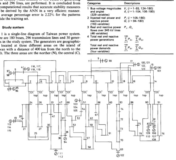
To demonstrate the effectiveness of the proposed neural-network approach, eigenvalue analyses of Taiwan power system, which consists of 180 buses, 30 generating units and 296 lines, are performed. It is concluded from the computational results that accurate stability measures can be derived by the ANN in a very efficient manner. The average percentage error is 2.22% for the patterns outside the training set.

2 Study system

Fig. 1 is a single-line diagram of Taiwan power system. There are 180 buses, 296 transmission lines and 30 gener- ators in the study system. The generators are geographic- ally located at three different areas on the island of Taiwan with a distance of 400 km from the north to the south. The three areas are the norther (N), the central (C),

I

94

6,111

1 1 2

Fig. 1 Single-line diagram of Taiwan power system

and the southern (S). Heavy interarea line flows may cause low-frequency oscillations if there is insufficient damping [l]. It is thus desirable to evaluate small-signal stability measures in system operation. Table 1 lists the buses in the study system. Note that nuclear units and some hydro-electric units are dispatched as base load units while thermal units are used for load-following.

Table 1 : Summary of system buses

For the purpose of eigenvalue analysis, we need the system variables as listed in Table 2. Note that other variables such as voltage-angle separation between two buses can also be included in Table 2. However, these variables are not considered in the present work because

Table 2: System variables required for eigenvalue analysis Categories Descriptions 1 Bus-voltage magnitudes and angles (329 variables) reactive power (1 63 variables) 3 Real and reactive power

flows over 345 kV lines (46 variables) 4 Total real and reactive

power generations Total real and reactive power demands (four variables)

2 Injected real power and

V , ( i = 1-93, 124-1 80) 6, (i = 1-1 04, 106-1 80) P, ( i = 105-1 80) a, ( i = 94-1 80) p,. 0, 180 1 8 0

Bus t w e Bus numbei

Swing bus 105

PV buses (base-load units) 94-1 04 PV buses (load-following units) 106-123 PO buses (345 kV. north area) 1-7 PQ buses (345 kV, centre area) 8-1 3 PO buses (345 kV. south area) 14-18 PO buses (69 kV) 124-1 80 PO buses (161 kV) 19-93

I E E Proc.-Gener. Transm. Distrib., Vol. 141, No. 3, M a y 1994

.

2

120,121

?

.

11 99

,

;;;>

ploo

101 110 107 76 6 1 0 2

they are functions (e.g. difference or sum of two variables)

of the variables in Table 2 and these functions can be accomplished by the neurons in the hidden and output layers of the neural network.

Note that the total number of system variables is 542, system variables being denoted by Sj ( j = 1, 2,

. . .

, 542). Certain constant parameters such as generator react- ances, time constants, exciter constants and line react- ances do not change with system-loading conditions. They are therefore not selected as potential candidates for neural-network inputs. In fact, these constant parameters can be dealt with using the bias terms of neurons in neural-network implementations. However, in conven- tional time-domain and frequency-domain approaches, both these constant parameters and the system variables are required for digital simulations or eigenvalue computations.

In Section 3, an artificial-neural-network approach

(3)

will be introduced to evaluate system-stability measures without the laborious task of digital simulation or eigenvalue computations.

3 Artificial-neural-network approach

As shown in Fig. 2, the design of ANN invohes four major steps: training-set creation. feature selection, training and testing.

unit-commitment routine economic-dispatch routine power-flow-analysis routine clustering ANN

1 training set creotion

multilayer feedforwarc ANN 3 training (generalised delta rule) L testing multilayer feedforward ANN Fig. 2 Neural-network design procedures

The first step in neural-network design is to create the training patterns in the training set. To do this, the his- torical operating records of Taiwan power system are compiled. The collected data sets consist of bus loads, bus voltages, line flows and generation patterns which characterise system operating conditions. The compiled operating point is referred to as the base operating point. To describe the system more adequately, we need other operating points in addition to these compiled base operating points. This is acheived by randomly varying each bus load in the base operating point over a wide range of *20%. Some derived operating points can be obtained by executing unit-commitment, economic-dispatch and power-flow-analysis routines for each perturbed loading condition. We use this method to generate 200 operating points, among which 120 points are randomly chosen as the training patterns. The remaining 80 points will be used as testing patterns. Note that the generation of these patterns is achieved by limited variation of the base operating point. Therefore, these patterns are somewhat related. Each operating point (including base operating points and derived operating points) is described by a

feedforward ANN. As a result, each training pattern ti in the training set for the multilayer feedforward ANN is described by the input (Xi)-output (ai) pair as follows

t; = ( X i , ai) (1)

where ui is the real part of the eigenvalues for the worst- damped modes under the operating point described by

x .

If this set of training patterns is directly applied to train the multilayer feedforward ANN using the generalised delta rule [SI, one may face the problem of local minima and slow convergence. This is caused by the huge number of neurons and unknown connection weights which are proportional to the number of inputs (542 in the present case). Thus it is desirable to reduce the number of inputs to the ANN so that the resultant state vector Xi = [xi,, x i 2 ,

. . .

, xic] will include only those G system variables (Sl, S,,

. . .

, S,) which are essential for stability-measure evaluation by the ANN. With these reduced state vectors Xi and training patterns

t ;

=(A,;,

a) (2) at hand, it is expected that the multilayer feedforward ANN can be efficiently trained by using the generalised delta rule in the training phase. Finally, in the testing phase, the trained multilayer feedforward ANN must yield accurate stability measures for operating points both in and outside the training set. In Section 4, a clustering ANN will be presented to reduce system variables and to select key features for stability evaluation. 4

The basic principle for a clustering ANN [SI is to group the total N ( N = 542) system variables (SI, S, , . .

.

, S,.,) into G clusters such that the variables in a cluster have similar characteristics. We then pick out one representative variable in a cluster as the feature for this cluster. This will reduce the number of system variables from

N

to G . For the purpose of feature selection using the clus- tering ANN, M = 120 training patterns (ti = (Xi, oi), i = 1, 2, ,

.

. , 120) are created.

Clustering A N N f o r f e a t u r e selection

I

2,

. . .

, M ) at hand, form the matrix X'

With the state vectors X ; = [x:,, xi2, ..., xi,.,] (i = I ,

r

X'I 2 . . . x i ,

,.,

1

+ operating point I

. . .

X i 2 XMZ ... t

t

. . .

X i 2 XMZ ... t

t

variable 1 variable 2 variable N

(SI) (S,) (S,.,)

state vector X' which comprises the 542 system variables as listed in Table 2. These 542 variables S j ( j = I , 2,

. . .

, 542) form the set of potential candidates for the inputs to the multilayer feedforward ANN. For the convenience of later discussions, we use the row vector X ; = [xil, xiz,

. . .

, xi, 542] to represent the state vector for the ith oper-

ating point. Note that x i j is the value for system variable

Sj under ith operating condition.

To evaluate the damping characteristic for each operating point, the eigenvalues for the electromechanical modes are computed using the AESOPS program [2]. The real part of the eigenvalues for the worst-damped modes a is a good measure of small-signal stability. Therefore, we select a as the output of the multilayer 200

(3) It is observed that row i of matrix X' contains the values for N ( = 542) system variables (S,, S, ,

. . .

, S,.,) at operating point i while column j of matrix X' consists of the

S j variables in the M ( = 120) training patterns. Define the column vector Y j = [ x i j ,

x i j ,

..., xLjIT = [ y l j , y Z j , ...,

yMjIT. Then the 542 system variables S j ( j = 1, 2, ..., 542)

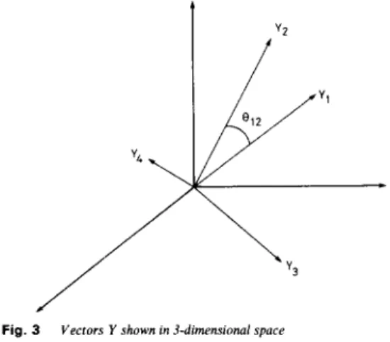
can be clustered based on these vectors Y j . Those system variables with similar vectors Y j will be grouped in a cluster. As shown in Fig. 3, two vectors Y , and Y , which are similar to each other will have a small angle between them. We can therefore put a group of these similar vectors in a cluster. To do this, define the cosine value of the angle 8,k between two vectors and Y, as

c o s ~ j k = ~ I ; . r , ) / ( l r ; l

IKl)

(4) I E E Proc.-Gener. Transm. Distrih., Vol. 141, No. 3, M a y 1994

(4)

This cosine value can be used to evaluate the degree of similarity between two vectors. If cos (e,,) is greater than a specified threshold p r , the two vectors and

&

are

Fig. 3 Vectors Y shown in 3-dimensional space

regarded as two similar vectors and are put in the same cluster. Details of the clustering algorithm are described as follows.

Step I : Let system variable S1 belong to cluster 1 and let the cluster vector for cluster 1, C , = [ell, czl,

...,

c M 1 I T , be equal to column vector Y , , i.e.

cil = y i , i = 1, 2, ..., M ( 5 ) Set initial countj = 0, G = 1.

Step 2: Increase j by one.

Step 3: Compute the cosine value D , between vectors

Y j and C,(g = 1, 2,

. . .

, C).

Let

D,, = max

(D,)

(7)

U

If D,, < pr (a specified threshold), the present vector Y j is far from any existing cluster vectors and we have to create a new cluster for system variable S j . Go to step 5.

If De, > pr , the present vector Y j is close to cluster vector Cgy of cluster g,,, and system variable Sj should be assigned to cluster gm. Proceed to step 4.

Step 4: If vector Y j has not been presented before, let system variable S j be grouped in cluster g, and update the cluster vector C,, = [c,,,, cZ,,, ..., cM,,JT as follows

(8)

where k,, is the number of system variables in cluster g,

.

Go to step 6. If vector Y j has been presented before and variable S j has been grouped in cluster g m go to step 6.

If vector Y j has been presented before and variable S j has been grouped in a different cluster gm. move system variable S j to cluster g, and execute the update formulae

tiel = yij

+

cie, k,, i = 1, 2,

. .

., M

cigm = y i j

+

cign k,, i = 1, 2,

. . .

, M

ciemn. = -yi,

+

ciem..kg,,,. i = 1, 2,

. . .

, M

(9) (10) where kern: is the number of system variables in cluster g,.. In this case, this a move in cluster elements. Go to step 6.

I E E P r o c . - G e w . Tranym. Distrib., Vol. 141, No. 3, May 19Y4

Step 5: Create a new cluster gn for system variable S j with the cluster vector C,, = [c,,. , c Z g n , .

. .

, cM,JT where

cign=yij i = l , 2

,...,

M (11)

Increase G by one and go to step 6.

Step 6: If j = N , proceed to step 7; otherwise, go to

step 2.

Step 7: If there is any more in cluster elements in the preceeding N iterations, reset j to zero and proceed to step 2. Otherwise, go to step 8.

Step 8: For each cluster g, find a system variable S, whose column vector Y , is closest to the cluster vector

C, , i.e.

for any S j in cluster g. Let system variable S , be the feature variable for cluster g. Print out the system variables and feature variable for each cluster and stop. 5 M u l t i l a y e r f e e d f o r w a r d ANN f o r eigenvalue

analysis

Using the clustering ANN as described in Section 4, the 542 system variables can be grouped into G clusters. By selecting one representative feature S, for each cluster g, a total of C (G = 14 for our study system) features can be derived. These G feature variables S , (g = 1, 2, . . . , 14) will be employed as the inputs to the multilayer feed- forward ANN as shown in Fig. 4 [6] to conduct eigen- value analysis. output layer hidden layer hidden layer input layer 51 %

. . .

s G 1

Fig. 4 Multilayerfeedforward neural network

The nodes in the input layer receive input signals from the outside world and directly pass the signals to the nodes in the next layer. The node in the output layer provides the desired real part of the eigenvalues for the worst-damped modes (U). In addition to the input layer

and the output layer, we need one or more hidden layers. The nodes in the hidden layers take signals from the input layer and send their outputs to the nodes in the next layer when computations within the nodes have

(5)

been completed. In this work, two hidden layers with 28 hidden units at each layer are used. It is noted that we need at least two hidden layers to cover all possible kinds of training pattern in the training set [7]. As for the number of hidden units per layer, an empirical figure of twice the number of inputs has been recommended [3]. In the present work, a neural network of 28 hidden units has been found to yield satisfactory results.

Before the neural network can be used to yield the desired eigenvalue real part, the connection weights must be determined. The process of determining the connection weights is usually referred to as the training process.

In the training process, 120 different operating condi- tions are considered covering a system load from 6200 MW to 9200 MW for the study system. The test patterns are also selected from the same range since the system load is within the range for the study period. However, the ANN can be applied to generate the solution for a pattern outside the range. This solution speed i s similar, but the accuracy may be not as good when the system load is remote from the specified range. For each operating condition p , the values for the G features S ,

(g = 1, 2,

...,

G), i.e., xplr x p z . ..., and x p G are first recorded and the real part of the eigenvalues for the worst-damped modes up is computed by using the AESOPS program. Thus the training pattern p is described by

t, = {(input

PI,

(output

P I )

= {(X,I. xp2 > '. ' 3 X,C)' (up)) (13)

where xpg is the value of the system variable S , for train- ing pattern p .

A commonly used approach to training the multilayer feedforward ANN is the generalised delta rule [SI. In which the connection weights are updated in order to minimise the sum-of-squares errors between the desired output and the actual output. Details of the update formula can be found in Reference 6.

expected since a greater threshold in step 3 of the clus- tering algorithm will tend to create more new clusters. A proper value of p r must be selected such that the resultant features will yield fewest errors in the testing phase when they are applied as inputs to the multilayer feedforward ANN to evaluate system eigenvalues. The issue will be addressed below.

To give a clear picture on how the system variables are clustered in different groups, Table 4 lists the system variables in each cluster for pr = 0.9.

Tabla 4: Svstem variables in each cluster ( D . = 0.90) Cluster Feature System variables

1 2 3 4 5 6 7 8 9 1 0 11 12 13 14 V , , i = 1-93, 124-1 80 6,, i = 51,54-67,69,85,95-99,103,104, 149-1 59,162,164,173-1 75 P,, i = 105,108-1 10,113-1 15,124-1 80 Q,, i = 99,124-1 80 P l l . Z ' P L I . e . ~ P L 2 . 5 ' P L 3 . 5 ~ P L 3 . 7 , PM.6. PL5,17 * PL,O. 1 1 . PL,,, 1 2 I PL,.3.15, PL15.18,

Q L s , 3 3 , Q t , o , 7 1 IPGr IPL 1 EQ,

140,141,145, 148 Q ' , , , l 3 6 , , i = 1 4 . 1 ~ 1 8 . 3 6 , 3 8 , 1 0 6 . 1 0 7 , 1 2 5 . 1 3 2 . 6,, i = 1-1 3,19-35,40-50.70-84. 86-94. 102. 108-1 19, 124. 126-1 31, 133-1 35,138, 142. 144,146-1 47, 160-1 63,165-1 7 2 , 1 7 6 1 80 PL,, 1 3 1 P L 7 . 1 3 I PL8.11, P L 8 . 1 3 I PL,,, 1 3 , p L 8 , j , * 'L8.13, Q L t l , ? 6 * 'L71, 1 8 6 , . i ~ 3 9 . 5 2 , 5 3 , l 0 0 , l 0 1 , 1 3 6 , 137,143 P , . i = 106,107,120-1 23, Q L 4 , . , P,,,, 1 7 ,

To examine the physical significance of the clustering results, Table 1 lists the 345 kV buses in the three areas of Taiwan. Since the excess power in the northern area or the southern area must be transmitted to other areas through the 345 kV trunk lines, the 345 kV buses in one area can be regarded as belonging to the same coherent group. In addition, the bus-voltage angles are important indicators for system stability. Therefore, it is expected that the bus-voltage angles in one area are grouped in the cluster. This observation is confirmed by the clustering results in Table 4. The voltage angles in the north ( h l , h , ,

. . .

, 6,) are grouped in cluster 3. The voltage angles in the centre

(a,, a,,

. . .

, h I 3 ) are also grouped in cluster 3 while

the voltage angles in the south (6,,,

a,,,

hI8) are grouped in cluster 2. Although there is a minor exception

(al5),

the correlation between the clustering results and the coherent groups can generally be established. Note that the variances of voltage magnitudes are very small (within 0.001). Therefore the variables for the voltage magnitudes are in the same cluster in Table 4. On the other hand, the variances of phase angles, real powers IEE Proc.-Gener. Transm. Distrib., Vol. 141, No. 3, May 1994

(6)

and reactive powers are about 0.45, 1.3 and 0.2, respec- tively, these are greater than those for the voltage magnitudes. These system variables therefore belong to different clusters (the variances of eigenvalues are within 0.000 24).

After the features have been selected, they are used as the inputs to the multilayer feedforward ANN which are trained using the 120 training patterns in the training set. The learning rate q and momentum constant a used in this work are 0.5 and 0.8, respectively. The resultant ANN is tested using the 120 training patterns in the training set and 80 other patterns outside the training set. To examine neural-network training and testing results, define:

Average percentage error for the training patterns in the training set

2 0 r

-L

:

10- U where t, and 0, are the desired and computed output ( U ) of the ANN, respectively, when pattern n in the training set is applied.

Maximum percentage error for the training patterns in the training set

20 -!

g

1 0 - i Y t" - 0" 1 2 0 E,,,, = max

1 t

,

I

x 100% " = l -

Average percentage error for the patterns outside the training set

where t , and 0, are the desired and computed output ( U )

of the ANN, respectively, when pattern n outside the training set is applied.

Maximum percentage error for the patterns outside the training set

80

E,,,* = max

-

- On x 100%

n = l

I

t"

I

The average percentage error E,,,, and maximum percentage error EMMAXI are depicted in Figs. 5-7 as func- tions of the number of iterations in the training process

I

500 1MM 1500 2MM

- 1

OO

iteraton

Fig. 5 Average percentage error E,,,, and maximum percentage error E,,,, in the training process ( p , = 0.85)

for p, = 0.85, pt = 0.9 and pr = 0.95, respectively. Note

that, in one iteration, the 120 training patterns in the training set are all presented once. The training times for ZOO0 iterations on a Sun IV-60 Workstation and the IEE Proc.-Gener Transm. Distrib., Vol. 141, No. 3, M a y I994

errors from testing the resultant ANN are compared in Table 5.

Table 5 : Comparison of the training for 2000 iterations and oercentaae errors for different threshold D.

Threshold Number Training Average Maximum

P , of time for error error

features 2000

(cluster iterations EA,,, EAYE2 E,,,, E M l X 2

min 76 "A, 'X, "A,

0.85 10 56.3 2.43 2.87 8.91 13

0.9 14 60 1.51 2.22 5.29 7.69

0.95 28 73.6 0.99 2.96 5.46 10.8

OO

-

500 loo0 1500 20w

iteration

Fig. 6 Average percentage error E A V E L and maximum percentage error E,,,, in the training process (p, = 0.9)

I I

0 500 1000 1500 2030

iterat ion

Fig. 7 Average percentage error E,,,, and maximum percentage error E,,,, in the trainrny process (p, = 0.95)

From the results in Figs. 5-7 and Table 5, the following observations are in order.

The number of connection weights in the ANN increases with increasing number of inputs (features). Therefore, the required training time will increase as the number of inputs to the ANN is increased.

Among the three thresholds used in the present work, a value of p, = 0.85 will result in an ANN with greatest percentage errors. The average percentage error reaches 2.87% while the maximum percentage error reaches 13%)

for those patterns which are not in the training set. It seems that a large threshold will result in fewer features than are required fully to describe the small-signal stability of the study system.

If the threshold is increased to 0.9, the clustering ANN recommends that we use 14 inputs for the multilayer feedforward ANN. In this case, the average percentage

(7)

error EAVEl and maximum percentage error EuAxl for the patterns in the training set are 1.51% and 5.29%, respectively, while those for the patterns outside the training set are 2.22% and 7.69%, respectively. A con- siderable improvement in ANN performance over the case of p, = 0.85 is achieved. In normal operation of Taiwan power system, the real parts of the electromechanical mode eigenvalues range from -0.1 to -0.2. In this case, a error of less than 10% is acceptable from the viewpoint of stability assessment.

If the threshold is further increased to 0.95 and the number of features increased to 28, no significant improvements in ANN performance can be made. In fact, the maximum percentage errors for the present case are greater than those in the case of pt = 0.9. A possible reason for the deterioration of performance in this case is that some minor variables are included as features of the system, causing interactions with major system features. A value of 0.9 seems to be a proper choice for the thresh- old in our study system. Note that the threshold value is system dependent and a proper value can only be achieved by a trial-and-error process.

Once the multilayer feedforward ANN has been trained, it can be employed to generate the desired eigenvalue real part very efficiently. The average CPU time required to obtain an answer on a Sun IV-60 Work- station is about 0.05 s. It is expected that the neural networks designed can provide on-line operational aids to system operators.

7 Conclusions

In this paper we propose to use artificial neural networks to perform eigenvalue analysis of Taiwan power system. A clustering ANN is first developed to select those fea- tures from system variables which can be used to characterise system stability. These features are then employed as the inputs to a multilayer feedforward ANN which is designed to evaluate system stability based on the input signals. The multilayer feedforward ANN has been trained using 120 training patterns in the training set and tested with other 80 patterns outside the training set. Results from eigenvalue analyses of Taiwan power system reveal that an average percentage error of 2.22% can be achieved for the patterns outside the training set.

In the present work, the training patterns used in the training phase and the test patterns used in the test phase cover a wide range of bus loads and generation profile. Since line switchings are rare events in normal operation of the Taiwan power system, the change of system topology due to such events is not considered in this paper. To take this factor into account, additional system variables which characterise system topology must be employed as the inputs to the neural networks.

For systems larger than Taiwan power system such as the US West Coast System, one may be interested in more than one mode. In this case, we need more than one output from the ANN. However, the techniques remains the same.

8 References

I HSU, Y.Y., SHYUE, S.W., and SU, C.C.: ‘Low frequency oscil-

lations in longitudinal power systems: experience with dynamic stability of Taiwan power system’, I E E E Trans., 1987, PWRSZ, pp. 92-100

2 BYERLY, R.T., BENNON, R.J., and SHERMAN, D.E.: ‘Eigen- value analysis of synchronising power flow oscillations in large electric power systems’, I E E E Trans., 1982, PAS-101, pp. 235-243 3 SOBAJIC, D.J., and PAO, Y.H.: ‘Artificial neural-net based

dynamic security assessment for electric power systems’, I E E E Trans., 1989, PWRS-4, pp. 220-228

4 MORI, H.: ‘An artificial neural-net based method for estimating power system dynamic stability index’. First international forum on Applications of Neural Networks to Power Systems, Seattle, USA. July 1991,pp. 127-133

5 MORI, H.. and TAMURA, S . : ‘An artificial neural net based tech- nique for power system dynamic stability with the Kohonen Model’,

IEEE Trans., 1992, PWRS-7, pp. 856-864

6 RUMELHART, D.E., HINTON, G.E.. and WILLIAMS, R.J.: ‘Learning internal representations by error propagation’, in RUMELHART, D.E., and McCLELLAND, J.L. (Eds.): ‘Parallel distribution processing’. Vol. 1. Chap. 8

7 LIPPMANN, R.P.: ‘An introduction to computing with neural nets’, I E E E ASSP Mug.. 1987, pp. 4-22

8 PAO, Y.H.: ‘Adaptive pattern recognition and neural networks’ (Addison-Wesley Publishing Co., 1989). Appendix B

9 SOBAJIC, D.J., PAO, Y.H., and DOLCE, J.: ‘Real-time security monitoring of electric power systems using parallel associative mem- ories‘. IEEE international symposium on Circuit and Systems, New Orleans, USA, May 1990, pp. 2929-2932

IO WEERASOORIYA, S., and EL-SHARKAWI, M.A.: ‘Use of Karhunen-Loeve expansion in training neural network for static security assessment’. First international forum on Applications of Neural Networks to Power Systems, Seattle, USA, July 1991, pp. 59-64