Non-Location-Based Mobile Sensor Relocation in a Hybrid Static-Mobile Wireless
Sensor Network
Fang-Jing Wu, Hsiu-Chi Hsu, and Yu-Chee Tseng Department of Computer Science
National Chiao-Tung University Hsin-Chu, Taiwan
{fangjing, hchsu, yctseng}@cs.nctu.edu.tw
Chi-Fu Huang
Department of Computer Science and Information Engineering National Chung Cheng University
Chia-Yi, Taiwan [email protected]
Abstract
An inherent concern for a wireless sensor network (WSN) is the unbalanced energy consumption problem, where sen-sors closer to the sink are more likely to exhaust their energy faster than other nodes. To mitigate this problem, this paper considers including some resource-rich mobile nodes, called mobile data-pumps, to conduct data relaying from static sensors to the sink. The network thus becomes a two-tier network, with the original static sensors at the low tier and data-pumps at both low and high tiers. We propose a novel distributed navigation protocol that does not rely on any location information of sensor nodes to relocate data-pumps to meet both goals of connectivity and load balance. The main idea is a concept called virtual Voronoi cells, which can help data-pumps to locally balance their loads using the underlaying low-tier topology and thus significantly balance energy consumption of sensors. Simulation results are presented to verify the effectiveness of our result.
Keywords: load balance, mobile computing, mobile sensor, pervasive computing, wireless sensor network.
1. Introduction
The progress of embedded micro-sensing MEMS and wireless technologies has made the success of wireless sensor networks (WSNs). A WSN is usually composed of a sink and a large number of sensors, each capable of collecting environmental information. Research issues for WSNs, such as deployment [15], [21], energy-efficient MAC [7], [11], and data aggregation [3], have been intensively studied.
Sensor deployment is a critical issue for WSNs. A suc-cessful deployment must guarantee both connectivity and coverage. The former is to ensure that sensory data can be delivered to the sink, and the latter is to ensure that the whole sensing field is fully monitored. Another big challenge is the energy unbalanced problem, where it is known that sensors closer to the sink are likely to consume their energy much
faster than other nodes; a lot of works have tried to address this issue [1]–[4].
Recently, researchers have proposed to add resource-richer mobile nodes to help relieve the energy unbalanced problem. In [8], [9], [12], [13], [17], [18], [20], a set of mobile collectors are used to move along pre-planned paths to collect data from static sensors. The collection process can be single-hop [9], [13], [20] or multi-hop [8], [12], [17], [18]. While such approaches can balance the energy consumption of sensors, moving these collectors may cause long delays, thus harming real-time applications. To relieve this limitation, [19] proposes a two-tier architecture, where the low tier consists of typical sensor nodes and the high tier consists of mobile data-pumps, called syphons, each with a long-range and a range wireless interfaces. The short-range ones can communicate with the low-tier network. The goal is to design a range-free protocol to help these syphons to move around to form a connected syphon tree rooted at the sink by those long-range interfaces. The low-tier nodes can first relay their data to the nearest syphons and then the syphon tree can quickly relay these data to the sink. In this way, the energy requirement of low-tier nodes is relaxed.
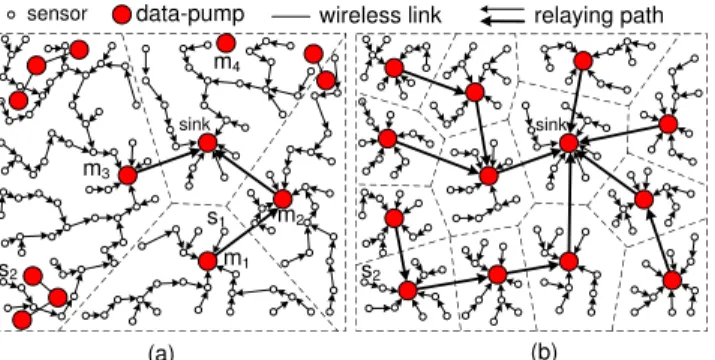
In this work, we adopt the same two-tier architecture as in [19]. However, we observe that the design of [19] does not try to balance the loads of syphons (i.e., the numbers of sensors served by syphons). Note that unbalanced loads of syphons will also affect the energy consumption, and thus the lifetime, of both high- and low-tier nodes. To resolve this problem, we propose a novel range-free relocation protocol based on a virtual Voronoi cell concept. We assume no loca-tion informaloca-tion for syphons, and nor for low-tier sensors. The only assumption is that the initial deployment of low-tier sensors should be dense enough to form a connected network with the sink. Initially, syphons may or may not be connected with the sink. Figure 1(a) gives an example, where the data of sensor s1 is relayed by m1 and m2, and that of sensor s2 needs to go long way to m3 and then to the sink. If we can properly relocate syphons as shown in Figure 1(b), then s2 can quickly relay its data via syphons. Relocating syphons needs to address both connectivity and
2009 Third International Conference on Sensor Technologies and Applications
data-pump
sensor relaying path
sink wireless link (a) (b) m1 m2 m3 m4 sink s1 s2 s2
Figure 1. An example of data collection scenario in a WSN: (a) the initial deployment (b) after relocation of data-pumps.
load balance. Connectivity needs to make sure that the high-tier network is not partitioned, while load balance is to make sure that each syphon serves the similar number of sensors. We successfully use virtual Voronoi cells to navigate syphons to achieve both goals simultaneously in a distributed manner. The navigation part is achieved relying on the underlaying low-tier topology.
Several existing works have addressed mobile sensor issues, but focused on different concerns. In [5], [22], mobile sensors are relocated based on the virtual forces. The work [14] uses the Voronoi diagram to detect coverage holes and relocates mobile sensors to cover these holes. These works [5], [14], [22] all assume that location information is avail-able. How to use the minimum number of mobile sensors to guarantee coverage and connectivity is discussed in [15], [16]. On the contrarily in our work, mobile sensors serve as the high-tier network under our two-tier architecture.
The rest of this paper is organized as follows. Section 2 formally defines our problem. The proposed distributed protocol is in Section 3. Section 4 shows our simulation results, and Section 5 concludes this paper.
2. Network Model and Problem Definition
In a sensing field F, we are given a two-tier network with a static sink m0, a set of static sensors S = {s1, s2, . . . , sn}, and a set of mobile data-pumps M = {m1, m2, . . . , me} (i.e., syphons). We assume that there are much more statics sensors than data-pumps, i.e., e ¿ n. Every node (sink, static sensors, and data-pumps) has a short-range antenna with a transmission distance rc. Each of the sink and data-pumps has a long-range antenna with a transmission distance Rc. Short-range antennas can only communicate with short-range antennas, and so are long-short-range antennas. The former forms the low-tier network, and the latter forms the high-tier network. Sink m0is a special data-pump which can not move. Our goal is to utilize the resource-richer data-pumps to help relay the sensory data from static sensors to m0.The problem if formulated as follows. Initially, all S and M are randomly deployed in F. Deployment of S is assumed to be dense enough so that the low-tier network is always connected. Deployment of M is sparse and thus the high-tier network could be partitioned. A data-pump that is connected to m0in the high-tier network is called attached, and is unattached otherwise. We assume no knowledge about the location of any node in S and M. Data collection is conducted by the cooperation of S and M. A si ∈ S can first send its sensory data, along the low-tier network, to the nearest attached pump, called the master data-pump χ(si). Then χ(si) can relay the data, via the high-tier network, to m0. Let C(mi) = {sj|χ(sj) = mi}, the set of sensors served by mi, called mi’s virtual Voronoi cell (‘cell’ for short). Our goal is to design a distributed range-free relocation protocol for data-pumps to achieve both connectivity and load balance. The connectivity requirement is to enforce all data-pumps to remain attached to m0 after relocation, while the load balance requirement is to keep the sizes of virtual Voronoi cells as similar as possible under all possible combinations of |M| and |S|. Note that the solution should be ‘range-free’ in the sense that navigating theses data-pumps can not rely on any geographic locations.
We propose two metrics to evaluate a relocation solution, and our goal is to minimize the two metrics: (i) load balance metric: max∀i,j{|C(mi)|−|C(mj)|} and (ii) radius metric: max∀i,j{R(mi) − R(mj)}, where R(mi) is the (low-tier) radius of mi’s virtual Voronoi cell centered at mi. Figure 1(a) and Figure 1(b) are examples before and after relocating M, respectively. Note that an unattached data-pump makes no contribution to relaying sensing data, because it is partitioned from the main part of the high-tier network.
3. Distributed Data-Pump Relocation Protocol
Our protocol has two operational modes: balancing mode and connecting mode. An attached data-pump will enter the balancing mode, while an unattached data-pump will enter the connecting mode. Initially, only the sink is attached and all other data-pumps consider themselves unattached. After the relocation process starts, each attached data-pump will periodically announce an Attachment message. Once an unattached data-pump hearing an Attachment message, it consider itself attached and also periodically announce an At-tachment message. Under the balancing mode, a data-pump will try to move toward the center of its virtual Voronoi cell and push away from its neighboring data-pumps. Under the connecting mode, a data-pump will attempt to connect to an attached data-pump. Once an unattached data-pump becomes an attached one, it will remain attached until the protocol terminates. Next, we describe these two modes in details. At the end, we will discuss the synchronization issue.55 70 42 s1 68 data-pump sensor moving direction 1 349,D | ) ( |Cm1 70 44 s2 m 0 m1 m2 m3 m0 m1 m2 m3 (a) (b) wireless link 114
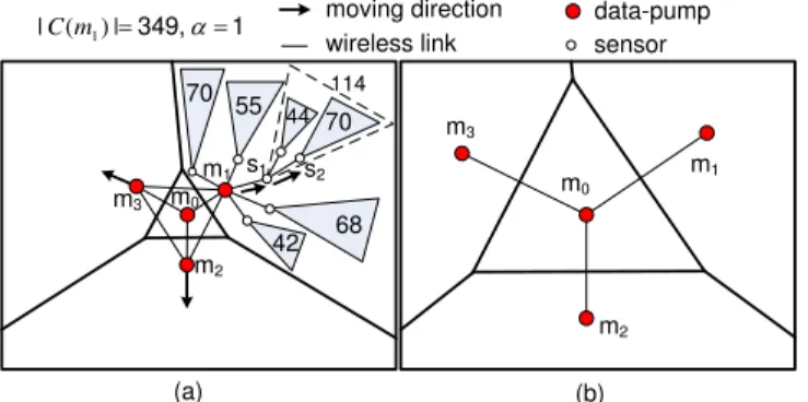
Figure 2. An example of relocating data-pumps.
3.1. Balancing Mode for Attached Data-Pumps
The main idea is to enforce each attached data-pump mi to move, based on local information, toward the ‘center’ of its current virtual Voronoi cell while keep attached. By so doing, load balance can be achieved eventually. Geometrically, F can be partitioned into multiple Voronoi cells based on attached data-pumps’ locations. However, since no location information is assumed, we will use the connectivity information among S as a clue to navigate data-pumps. For example, in Figure 2(a), m1can detect that it is not at the center of its current virtual Voronoi cell by forming an intra-cell tree rooted at itself. Our scheme will force m1 to move toward the child with the largest subtree, i.e., s1. After repeating this movement process several times, m1’s subtrees will reach certain equilibrium. Concurrently, m2 and m3 will conduct the same process. More importantly, this will repartition the virtual Voronoi cells. Figure 2(b) shows an ideal situation after several rounds.
Our protocol is designed as an iterative process with multiple rounds. Each round has four phases, during which a data-pump may make a movement. Phase 1 is to partition F into virtual Voronoi cells in a distributed manner. Phase 2 will decide each data-pump’s moving direction. Phase 3 will choose each data-pump’s parent to maintain the connectivity in the high-tier network. The actual movement and termination conditions are decided in phase 4. Phases among data-pumps need to be synchronized (refer to Sec 3.3).
Phase 1: Virtual cell construction. In this phase, each data-pump mi will compute its cell C(mi) by forming a tree Ti rooted at itself. Each sensor sj will maintain two variables: χ(sj) and h(sj) (hop count from mi to sj in Ti). Initially, χ(sj) = NULL and h(sj) = ∞. To start with, mi will broadcast a Cell(mi, h) message using its short-range antenna with h = 1 (standing for hop count). When any sj receives a Cell(mi, h) message, it will check the following conditions: (i) χ(sj) = NULL and (ii) h < h(sj). If any of the above conditions is true, sj will set χ(sj) = mi, set h(sj) = h, and broadcast a Cell(mi, h + 1) message. At the
end of Phase 1, each sensor will know its master data-pump. Phase 2: Cell center estimation. In this phase, each mi will try to identify the center sensor cn(mi) of its cell C(mi). Initially, mi will assume itself as the center, i.e., cn(mi) = mi, and broadcast a CEN T ER(cn(mi)) message around sensors in C(mi) to form a spanning tree rooted at itself. Each sensor sj will calculate the depth and the number of sensors of the subtree rooted at itself, denoted by djand nj, respectively. Then, each sensor sjcan compute a load index as follows:
εj = α · nj+ (1 − α) · dj,
where 0 ≤ α ≤ 1 is a weight to reflect the importance of our two metrics (i.e, the deviation among |C(mi)| and the deviation among R(mi)). Then, mi will run the following iterative process to update the center sensor cn(mi). The main idea can be imagined that mi throws an agent which is like a ball and will roll toward the center of C(mi) along the sensors with higher load index. Specifically, in each iteration, mi will try to update the center sensor cn(mi) by the child of cn(mi) with the highest load index, denoted by sc, if the following condition is satisfied: εεc0
c ≥ 1, where
ε0
c = α ·degree(cn(m(|C(mi)|−ni))−1c) + (1 − α) · (dmax+ h(sc, mi)) is
the estimation of the average load index for the remaining subtrees rooted at cn(mi)’s children excluding the subtree rooted at sc. Here, degree(cn(mi)) is the low-tier degree of cn(mi) (in terms of short-range antenna degree), dmaxis the maximum depth of subtrees rooted at mi’s children in the spanning tree except the subtree rooted at sc’s ancestor, and h(sc, mi) is the short-range antenna hop count from sc to mi along the spanning tree. Note that instead of reforming the spanning tree, we use εc
ε0
c to estimate if the loads between
the side of the subtree rooted at sc and the remaining side in C(mi) is balancing after mimove to sc’s position. Once mi updates cn(mi) = sc, it must memorize the history of cn(mi) to help relocate itself along the sequence of sensors in the history when moving. This completes one iteration. This process is repeated until there is no descent of cn(mi) can satisfy the above condition. Note that, this phase can be repeated more times for refining the center sensor cn(mi) of this cell. Figure 2 gives an example, where |C(m1)| = 349, and α = 1. Initially, m1 finds the subtree rooted at s1 with highest load index ε1 = 114 and updates cn(mi) = s1, because ε1
ε0 1 =
114
58.75 ≥ 1, where ε01 = 349−1144 = 58.75. Then, m1 repeatedly run this process until it finds εε20
2 < 1,
where ε2 = 70, and ε02= 349−702 = 139.5. Finally, m1 can identify the center sensor cn(m1) is s1.
Phases 3: Connectivity maintenance between mobile data-pumps. In this phase, each data-pump mi must choose an attached data-pump to be its parent, denoted by P (mi) for keeping attached. Specifically, mi must make sure that it can always hear the periodical Attachment message from P (mi) when moving. To achieve this goal, each
mi must choose the P (mi) with minimum cost(P (mi)) such that either the following rules can be satisfied: (i) H(P (mi)) < H(mi) or (ii) H(P (mi)) = H(mi) and H(P (P (mi))) < H(P (mi)), where H(mi), H(P (mi)), and H(P (P (mi))) are the minimum high-tier hop count from sink to mi, P (mi), and the parent of P (mi) in the high-tier network, respectively. Here, the cost(P (mi)) is defined by βNc
P (mi) + (1 − β)φ(P (mi), mi), where
Nc
P (mi) is the number of data-pumps whose parents are
P (mi), φ(P (mi), mi) is the received signal strength of the Attachment message from P (mi) to mi, and 0 ≤ β ≤ 1 is the weight to reflect the importance between Nc
P (mi)and
φ(P (mi), mi). Note that the smaller NP (mc i) will open up
an opportunity for data-pumps to span the larger-scale high-tier network served by them as much as possible, while the smaller φ(P (mi), mi) will open up an opportunity for data-pumps to move toward the position decided in phase 2 as far as possible under keeping the connectivity in the high-tier network.
Next, we detail the protocol as follows. Initially, sink must broadcast a message via the high-tier network to identify the H(mi) of each mi. Then, the sink must broadcast a Select Parent message via the high-tier network and wait for time period ∆tp to count Nsinkc . When a data-pump mi receives the first Select Parent message from another data-pump, denoted by mj, it will send a Become child message to mj, set P (mi) = mj, rebroadcast the Select Parent message, and wait for time period ∆tp. Once the mjreceives a Become child message from mi, it must update Nmcj by
Nc
mj + 1 and add mi into its children list L
c(m
j), where Lc(m
j) contains the data-pumps whose parents is mj. After a data-pump mi’s timer ∆tp is expired, miwill announce a Confirm Parent(mi, Nmci) message. When a data-pump mi
receives another Confirm Parent(mk, Nmck) message from a
neighboring data-pump mkwith cost(mk) < cost(mj), and mk is satisfied any one of the above rules, it will announce a Change Parent(mj, mk) message to change its parent mj by mk. On the other hand, when mj and mk receive the Change Parent(mj, mk) message from mi, they will update their children list, respectively.
Phases 4: Navigation by sensors. In this phase, each data-pump mi starts to move along the sequence of sensors in the history of cn(mi), denoted by Q, computed by phase 2 until the termination condition of this round has reached as follows.
1. If Q 6= ∅, mi will remove the first entry from Q, said sj, and announce a Navigation Request(sj) message via the low-tier network. Otherwise, this round is terminated.
2. When the sensor sj hears the Navigation Request(sj) message, it will repeatedly announce a Come Here(sj) message.
3. Once mi receives the Come Here(sj) message, it will try to find the moving direction toward sj by the following way. Initially, mi will set D1, . . . , DK directions
based on its local coordinate and then go and back between the current position and the position by moving toward Di direction for d units distance, respectively, to test the difference in received signal strength, where i = 1, . . . , K. Then, mi moves toward the direction with the maximum increasing difference in received signal strength by d units distance. This process will be repeated until mi can not find a direction with increasing received signal strength (it implies that mi is nearby the sj). Then, mi must send a Navigation Complete(sj) to sj to stop the announcement of Come Here(sj) message.
4. After mi moves to the position nearby the sj, it must check whether it sill can hear the Attachment messages from P (mi) and each mj ∈ Lc(mi). If so, it will go to step 1 for continuing to move. Otherwise, this round is terminated and mi must backtrack to the previous positions until the connectivity between mi and P (mi) and between mi and each mj ∈ Lc(mi) could be reconnected.
The above four phases will be repeatedly executed round by round until the maximum execution round has been reached. Note that the number of execution rounds will have an impact on the performance of load balance. We will use simulation to find a modest maximum execution round later.
3.2. Connecting Mode for Unattached Data-Pumps
The main idea of this mode is to enforce each unattached data-pump mi to move, based on the local information, toward the sink until it is attached. Specifically, each unattached data-pump miwill move toward the neighboring sensor with minimum sensor hop count from sink (in terms of short-range antenna hop count). After initial deployment, the sink will broadcast a message via the low-tier network to identify the h(sj, sink) for each sj, where h(sj, sink) is the sensor hop counts from sj to the sink in the low-tier network. Each unattached data-pump mi must periodically announce a Connection Request message via the low-tier network to query nearby sensors. When a sensor sj receives a Connection Request message from mi, it will reply a Connection Reply(h(sj, sink)) message to mi. According to the received Connection Reply messages, miwill request the sensor sjwith minimum h(sj, sink) to provide the nav-igation by announcing a Navnav-igation Request(sj) message via the low-tier network. Then, mi can move toward the sensor sj by running the same procedures in the step 2 and step 3 of the phases 4. This procedure is repeatedly executed by mi until it can hear the Attachment message from other attached data-pumps and then become an attached one. Once mi has became an attached data-pump, it must periodically announce an Attachment message and switch to the balancing mode until the maximum execution rounds has been reached.
3.3. Synchronization Between Phases
We suggest two possible approaches to synchronize the phases between data-pumps. The first one is that the phases switching is coordinated by the sink, while the second one is that each data-pump will set a timer for each phase to control the switching timing between phases.
For the first type synchronization, upon the network is re-quested to perform our protocol, the sink must first broadcast a Phase1-2 Start message via the high-tier network to in-form attached data-pumps to construct cells and estimate the centers of cells. When an attached data-pump mi receives the Phase1-2 Start message, it will rebroadcast this message via the high-tier network and then execute the phase 1 and phase 2. After mi has finished phase1 and phase 2, it will send a Phase1-2 End message to inform the sink. The sink must collect Phase1-2 End messages from all attached data-pumps and then broadcast a Phase3 Start message to inform data-pumps to execute phase 3. It is similar to the above procedures, the sink must wait until it knows that all data-pumps have finished the current phase and then trigger the next phase by broadcasting message in the high-tier network. Also, when an unattached data-pump has became an attached one, it must listen the synchronization messages from the sink to conduct the balancing mode.
For the second type synchronization, each data-pump will set a specified a timer for each phase. Upon the network is requested to execute our protocol, each attached data-pump mi will enter the phase 1 and start a timer Phases1 Timer. After the Phases1 Timer expired, mi will enter the phase 2 and also wait a timer for the current phases until the timer has expired. This process will be repeatedly phase by phase until the protocol is terminated. On the other hand, when an unattached data-pump mi becomes an attached one, it will immediately send Synchronization Request message to the neighboring data-pumps to query how long it should wait for entering the balancing mode to start a new round. When an attached data-pump receives a Synchronization Request message, it will reply a Synchronization Reply message with a time duration, based on the timers of the four phases in the balancing mode. After mi receives reply message from neighboring data-pumps, it will switch to the balancing mode until the maximum execution rounds has been reached.
4. Simulation Results
We randomly deploy 20000 sensors and 75 data-pumps in a disk-sharp field with a radius of Rf. The short-range antenna and the long-range antenna have transmission distances rc = 60 m and Rc = 240 m, respectively (we use WiFi and ZigBee as the reference here; the former has a transmission range of five times the latter [10]). We set the parameters both α (in phase 2) and β (in phase 3) as 0.5. Our simulation results are all from the average of
100 runs. We compare our protocol against the SODaR protocol proposed in [19] by the following two ways. The first one (denoted by ‘ours-only connecting mode’) is that data-pumps only can perform the connecting mode to achieve the same goal of the connectivity in the SODaR. The second one (denoted by ‘ours’) is that data-pumps can run two modes in our protocol to achieve the both goals of connectivity and load balance. In SODaR, each unattached data-pump mi must move along the circle composed of sensors with the same sensor hop counts from the sink as mi’s (in terms of short-range antenna hop count) to connect an attached data-pump. In our simulations, we use three metrics to evaluate the performance of ours and the SODaR as follows.
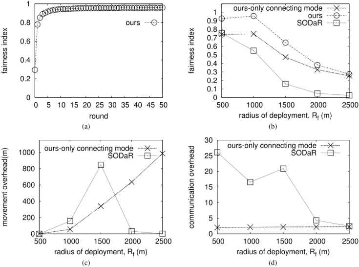
1. The quantification of the balance: we use the fairness index [6] to measure the deviation of data-pumps’ loads. Here, the fairness index is calculated by f (|C(m1)|, |C(m2)|, . . . , |C(me)|) = (Σ e i=1|C(mi)|)2 e·Σe i=1(|C(mi)|)2, where 0 ≤ f (|C(m1)|, |C(m2)|, . . . , |C(me)|) ≤ 1. Note that a protocol with the larger fairness index implies the less deviation of data-pumps’ loads (i.e., it is more balancing). 2. The movement overhead: we calculate the average moving distance of data-pumps in a protocol.
3. The communication overhead: we calculate the total number of messages exchanged in a protocol.
First, we find an adequate maximum execution round by observing the improvement in balance under different num-ber of execution rounds. Figure 3(a) shows the simulation result, where the fairness index only is slightly improvement after 10 rounds. Thus, we take the maximum execution round of our protocol by 30 rounds in the following simula-tions. Then, we investigate the impact of relocation protocols on balance under different radius of deployment. Figure 3(b) shows the result, where the fairness index is decreasing with the increasing of Rf. This is because the number of data-pumps is too less to span a large-scale high-tier network to balance the loads of data-pumps when Rf is larger. Note that our relocation protocol has prominent balance results even if only the connecting mode is conducted. Then, we focus on the goal of connectivity to compare the overheads of relocation protocols under different Rf. Figure 3(c) shows an interesting result on the movement overhead, where SODaR only can successfully work under some deployment cases (Rf is between 1000 and 2000) and results in higher movement overhead. This is because it may fail that an unattached pump in SODaR searches an attached data-pumps within a limited area. Note that the SODaR results in less movement overhead when Rf > 2000, because most data-pumps can not relocate themselves due to the SODaR fail. However, our connecting mode can always work out fine, and unattached data-pumps can quickly connect to the sink with less moving distance. Finally, in Figure 3(d) shows
0 0.2 0.4 0.6 0.8 1 0 5 10 15 20 25 30 35 40 45 50 fairness index round ours 1 0.9 0.8 0.7 0.6 0.5 0.4 0.3 0.2 0.1 0 500 1000 1500 2000 2500 fairness index radius of deployment, Rf (m) ours-only connecting mode
ours SODaR (a) (b) 0 200 400 600 800 1000 500 1000 1500 2000 2500 movement overhead(m) radius of deployment, Rf (m) ours-only connecting mode
SODaR 0 5 10 15 20 25 30 500 1000 1500 2000 2500 communication overhead radius of deployment, Rf (m) ours-only connecting mode
SODaR
(c) (d)
Figure 3. Simulation results.
the simulation result on the communication overhead, where our protocol is slightly increasing with the Rf increasing. Note that the probability that the SODaR can work is decreasing with the Rf increasing, so the communication overhead in SODaR decreases when Rf is increasing.
5. Conclusion and Future Work
To prolong network lifetime, this paper adopts a hybrid static-mobile WSN including resource-richer mobile data-pumps and static sensors to conduct data collection, where data-pumps have responsibility to help relay data from nearby sensors to the sink. We propose a distributed mobile data-pump relocation protocol to achieve the connectivity and load balance among mobile data-pumps such that the performance of data collection is improved. Without location information about sensors and mobile data-pumps, we use the connectivity among sensors as a clue to help relocation mobile data-pumps by themselves. Simulation results show
that our protocol can provide prominent load balance among mobile data-pumps Our future work will consider to relocate data-pumps when sensors have different traffic load such that data-pumps’ load could be balanced.
Acknowledgments
Y.-C. Tseng’s research is co-sponsored by MoE ATU Plan, by NSC grants 95-2221-E-009-058-MY3, 96-2218-E-009-004, 96-2219-E-007-008, 97-3114-E-009-001, 97-2221-E-009-142-MY3, and 97-2218-E-009-026, by MOEA under grant 94-EC-17-A-04-S1-044, by ITRI, Taiwan, and by III, Taiwan.
References
[1] A. Anandkumar, L. Tong, A. Swami, and A. Ephremides. Minimum cost data aggregation with localized processing for statistical inference. In Proc. IEEE INFOCOM, pages 780– 788, 2008.
[2] R. Cristescu, B. Beferull-lozano, and M. Vetterli. On network correlated data gathering. In Proc. IEEE INFOCOM, pages 2571–2582, 2004.
[3] K.-W. Fan, S. Liu, and P. Sinha. Structure-free data aggre-gation in sensor networks. IEEE Trans. Mobile Computing, 6(8):929–942, 2007.
[4] K.-W. Fan, S. Liu, and P. Sinha. Dynamic forwarding over tree-on-DAG for scalable data aggregation in sensor networks.
IEEE Trans. Mobile Computing, 6(10):1271–1284, 2008.
[5] N. Heo and P.K. Varshney. Energy-efficient deployment of intelligent mobile sensor networks. IEEE Trans. Systems,
Man, and Cybernetics–Part A, 35(1):78–92, 2005.
[6] R. K. Jain. The Art of Computer Systems Performance Analysis: Techniques for Experimental Design, Measurement, Simulation, and Modeling. John Wiley and Sons, New York,
1991.
[7] G. Lu, B. Krishnamachari, and C. S. Raghavendra. An adap-tive energy-efficient and low-latency MAC for data gathering in wireless sensor networks. In Proc. IEEE Int’l Parallel and
Distributed Processing Symp., 2004.
[8] M. Ma and Y. Yang. SenCar: an energy-efficient data gath-ering mechanism for large-scale multihop sensor networks.
IEEE Trans. Parallel and Distributed Systems, 18(10):1476–
1488, 2007.
[9] M. Ma and Y. Yang. Data gathering in wireless sensor networks with mobile collectors. Proc. IEEE Int’l Parallel
and Distributed Processing Symp., pages 1–9, 2008.
[10] T. Nolte, H. Hansson, and L. L. Bello. Wireless automotive communications. In Euromicro Conference on Real-Time
Systems, pages 35–38, 2005.
[11] M.-S. Pan and Y.-C. Tseng. Quick Convergecast in Zig-Bee Beacon-Enabled Tree-Based Wireless Sensor Networks.
Computer Comm., 31(5):999–1011, 2008.
[12] J. Rao and S. Biswas. Joint routing and navigation protocols for data harvesting in sensor networks. In Proc. IEEE Int’l
Conf. Mobile Ad Hoc and Sensor Systems, pages 143–152,
2008.
[13] J. Rao, T. Wu, and S. Biswas. Network-assisted sink navi-gation protocols for data harvesting in sensor networks. In
Proc. IEEE Wireless Comm. and Networking Conf., pages
2887–2892, 2008.
[14] G. Wang, G. Cao, and T.F.L. Porta. Movement-assisted sensor deployment. IEEE Trans. Mobile Computing, 5(6):640–652, 2006.
[15] Y.-C. Wang, C.-C. Hu, and Y.-C. Tseng. Efficient placement and dispatch of sensors in a wireless sensor network. IEEE
Trans. Mobile Computing, 7(2):262–274, 2008.
[16] Y.-C. Wang and Y.-C. Tseng. Distributed deployment schemes for mobile wireless sensor networks to ensure multilevel coverage. IEEE Trans. Parallel and Distributed Systems,
19(9):1280–1294, 2008.
[17] G. Xing, T. Wang, W. Jia, and M. Li. Rendezvous design algorithms for wireless sensor networks with a mobile base station. Proc. ACM Int’l Symp. Mobile Ad Hoc Networking
and Computing., pages 231–240, 2008.
[18] G. Xing, T. Wang, Z. Xie, and W. Jia. Rendezvous planning in wireless sensor networks with mobile elements. IEEE Trans.
Mobile Computing, 7(12):1430–1443, 2008.
[19] G. Yang, B. T. amd Daji Qiao, and W. Zhang. Sensor-aided overlay deployment and relocation for vast-scale sensor networks. In Proc. IEEE INFOCOM, pages 2216–2224, 2008. [20] M. Zhao, M. Ma, and Y. Yang. Mobile data gathering with space-division multiple access in wireless sensor networks.
Proc. IEEE INFOCOM, pages 1283–1291, 2008.
[21] Y. Zou and K. Chakrabarty. Sensor deployment and target lo-calization based on virtual forces. In Proc. IEEE INFOCOM, pages 1293– 1303, 2003.
[22] Y. Zou and K. Chakrabarty. Sensor deployment and target localization in distributed sensor networks. ACM Trans. Embedded Computing Systems, 3(1):61–91, 2004.