PDFF and H(infinity) Controller Design for PMSM Drive

(1)

Stone Cheng†_{, Yuan-Yong Huang, Hsin-Hung Chou, Chia-Ming Ting, Cheng-Min Chang, Ying-Min Chen} †_{Department of Mechanical Engineering, National Chiao-Tung University, Hsinchu, Taiwan, ROC} Mechatronics Control Dept., Intelligent Machinery Technology Div., MSL/ITRI, Hsinchu, Taiwan, ROC Abstract- This paper presents analysis, design and simulation of

velocity loop PDFF controllers and H∞ feedback controller for permanent magnetic synchronous motor (PMSM) in the AC servo system. PDFF and H∞_{control algorithm have its own capability of}

achieving good performance criteria such as dynamic reference tracking and load torque disturbance rejection. The PDFF is designed and analyzed in the forward loop to provide low frequency stiffness and overcome low-frequency disturbances like friction. While in the feedback loop, H∞ controller is designed to meet system robust stability with the existence of external disturbance and model perturbations. The proposed PDFF and H∞_{controllers are designed based on the transfer function of the}

poly-phase synchronous machine in the synchronous reference frame at field orientation control (FOC). The parameter variations, load changes, and set-point variations of synchronous machine are taking into consideration to study the dynamic performance.

Keywords: PMSM, H∞ feedback control, PDFF controller,

I. INTRODUCTION

The PMSM motor servo drive play an important role in industrial motion control applications including machine tools, factory automation and robotics in the low-to-medium power range. Several situations encountered in these applications: 1) Plant parameters such as load inertia and friction may vary during operation as the payload changes. 2) System bandwidth is limited by the presence of a tensional resonance of the mechanical system. 3) In AC servo motors, higher torque ripple and coupled dynamics with magnetic flux caused the nonlinearities in torque response and torque transients. 4) The set-point tracking capability in both dynamic and steady-state conditions and the load torque disturbance rejection capability are varying during applications. Several control techniques [1-7] have been developed to overcome these issues. Derived from generalized PID controller, the PDFF controller is allowing the user to eliminate overshoot and provide much more DC stiffness than PI by properly choosing the controller parameters. It is also known [8] that PDFF controller is less sensitive to plant parameter variations and its disturbance rejection characteristics are much better than that of the PI controller. Along with PDFF controller, H∞_{control theory is one of the}

successful algorithms for robust control problem in PMSM drive to provide better tolerance to disturbance and modeling uncertainties. In this paper, the H∞_{design procedure[4,9,10] is}

proposed and consists three main stages: 1) using weighting matrices W1 and W2 to shape the singular values of the nominal

plant follows the elementary open-loop shaping principles; 2) the normalized coprime factor H∞ problem is used to find a robust central controller stabilizing this shaped plant, and the

observer is obtained from the left coprimeness of the central controller; 3) the H parameter in the controller is used as a tradeoff between robust stability and performance.

II. MATHEMATICAL MODEL OF THE PMSM

The field orientation of the PMSM is defined as d-axis, and q-axis that leads the d-axis 90 electric degrees. In the d-q coordinates, the PMSM voltage-current and flux equations are shown as follows: d d d r q

v

=

Ri

+

λ ω λ

&

−

(1) q q q r d

v

=

Ri

+ −

λ ω λ

&

(2) d

L i

d d PM

λ

=

+

λ

(3) q

L i

q q

λ

=

(4)

Where vd and vq are voltages of the d, q axis; R is the stator

resistance; id and iq are the d, q axis stator currents; ωr is the

rotor speed; λd and λq are the d, q axis flux induced by the

currents of the d, q axis inductance; Ld and Lq are the q, d axis

inductances with the same value, and λPM the constant mutual

flux of the permanent magnet.

When the stator current vector is oriented perpendicular to the rotor magnetic field, the field-oriented control for PMSM yields id =0. In the case, the electromagnetic torque is in strict

positive proportion to iq:

3

4

e PM q T q

P

T

=

λ

i

=

K i

(5)

where P is the number of poles and KT is the motor torque

constant.

The mechanic motion equation is:

r e T q d r

d

T

K i

T

B

J

dt

ω

=

= +

+

(6)

where J is the moment of inertia; B is the viscous friction, and Td is the torque disturbance such as the load resistance, the

torque ripple and the resistance caused by nonlinear factors. III. DESIGN OF THE CONTROL SYSTEM A. Control Scheme

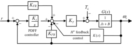
The proposed control scheme is presented in Fig. 1 where the nominal plant is G(s) = 1/(Js+B); K(s) is the velocity feedback controller designed by the loop shaping design procedure (LSDP) and the algebraic method, and the velocity lop controller is a PDFF controller. K(s) is used for attenuating the disturbance Td, and plant uncertainty, and the PDFF

controller is used as velocity loop adjuster to improve the low-frequency stiffness.

T. Sobh et al. (eds.), Novel Algorithms and Techniques in Telecommunications, Automation and Industrial Electronics, © Springer Science+Business Media B.V. 2008

PDFF and H

∞

Controller Design for PMSM Drive

(2)

Fig. 1 Control scheme B. Velocity Feedback Controller

In this paper, a continuous time control design approach based on H∞

-optimization control design is performed for a model of the PMSM system as seen from the digital computer control design approach. Consequently, performance is specified at the controller disturbance instants.

Minimum phase W1 and W2 are proper stable, real rational function denoted by RH∞.The left and right coprime

factorizations of W1GW2 are

M N

% %

_S−1 _S and

N M

_S _S−1 , respectively. Moreover, a doubly coprime factorization exists as follows: r r S l S l r r S S S l S l S S

X

Y

M

Y

M

Y

X

Y

I

N

M

N

X

N

X

N

M

−

⎡

⎤ ⎡

⎤

=

⎢

₋

⎥ ⎢

₋

⎥

⎣

%

⎦ ⎣

%

⎦

(7) where NS, MS, N%S, M%S, Xr, Yr, Xl, and Yl are over RH∞.

Then, the velocity controller K(s) is defined as follows:

1 2

( )

_v

( )

K s

=

W s K s W s

(8) Where _{( ) [} 1 _{] [}1 1 _] v r l r l K s ₌ X ₊H Y N− % − Y ₋H Y M− % _{and H is a}

unit over RH∞. With K(s) of (8), the velocity feedback loop is

internally stable. Moreover, Xr and Yr of Kv(s) in (8) play the

similar role as central controller although H in Kv(s) cannot be

0. According to this property, Xr and Yr can be designed using

the LSDP and H will be used to reject step and sinusoidal disturbance, as follows.

C. Design of Velocity Controller Using the LSDP and the Algebraic Method The first stage in the LSDP uses a pre-matrix W1 and/or a post-matrix W2 to shape the singular values of the nominal plant G as a desired open-loop shape GS = W2GW1. Constant or dynamic W1 andW2 are selected such that GS has no hidden

modes. Constant weighting matrices can improve the performance at low frequencies and increases the crossover frequency. Moreover, the dynamic W1 or W2 is used as the integral action with the phase-advance term for rejecting the input and output step disturbances. W1or W2 is selected as the diagonal matrix and each principal element is (s+φ)/s where φ >0 is lower than the crossover frequency. The integral action improves the performance at low frequencies, and the phase-advance term s+φ avoids the slope of the open-loop shaping at the crossover frequency more than -2, and adjusts the robustness in the feedback system. If φ is closer to the imaginary axis, the robustness is larger. The stage is the same

as the velocity controller herein.

[11-14] advocate an expression of coprime factor uncertainty in terms of additive stable perturbations to coprime factors of the nominal plant. Such a class of perturbations has advantages over additive or multiplicative unstructured uncertainty model. For example, the number of unstable zeros and poles may change as the plant is perturbed. The perturbed plant [See Fig. 2.] is written

1

(

_S _N

) (

_S _M

)

G

N

M

−

Δ

=

+ Δ ⋅

+ Δ

(9)

where the pair (MS, NS) is a normalized right coprime

factorization of GS, and ΔM and ΔN are stable, unknown transfer

functions representing the uncertainty and satisfying

N M

ε

∞

Δ

⎡

⎤

<

⎢

_Δ

⎥

⎣

⎦

, where

ε

( 0)

>

presents the stability margin.

In the second stage of the LSDP, the robust stabilization H∞

problem is applied to the normalized right coprime factorization of GS, and obtains a robust controller K∞

satisfying

Fig. 2 Right coprime factor robust stabilization problem

[

]

1

₍

₎

1 1 S S

M

−

I K G

−

K

I

ε

− ∞ ∞ _∞

+

≤

(10)

Suppose the shaped plant of GS has the minimal realization

(A, B, C, D). A central controller satisfying (10) is obtained as follows [15]: 2₍ T₎1 T₍ ₎ 2₍ T₎1 T T T A BF W ZC C DF W ZC K B X D

γ

−

γ

− ∞ ⎡ + + + − ⎤ =⎢ ⎥ ⎣ ⎦ (11) where _F_{= −}_S−1₍_{D C B X}T ₊ T ₎_;

_W

_{= +}

_I

₍

_XZ

₋

_γ

2

_I

₎

, and X and Z are the solutions to the two algebraic Riccati equations as follows: 1 1 1 1 (_{A BS D C X X A BS D C}₋ − T )T ₊ ( ₋ − T )₋_{XBS B X C R C}− T ₊ T − ₌0 (12) 1 1 1 1 (_{A BS D C Z Z A BS D C}₋ − T ) ₊ ( ₋ − T )T₋_{ZC R CZ BS B}T − ₊ − T₌0 (13) where R = I+DDT_{, and S = I+D}T_D.

If the plant is assumed to be strictly proper, i.e. D = 0, the realizations for the doubly coprime factorization can be presented as follows. 1 S

M

− S

N

M

Δ

N

−

K

_∞

−

− r ω 1 Js B+ ( ) G s r − − PDFF controller H ∞_feedback control K s( ) I K s KT KFB KFR − + + + + L T 238

(3)

0

S S

A BF B

M

F

I

N

C

+

⎡

⎤

⎡

_{⎤ ⎢}

₌

_⎥

⎢

_{⎥ ⎢}

_⎥

⎣

_{⎦ ⎢}

_⎥

⎣

⎦

(14)

0

S S

A QLC B QL

N

M

C

I

+

⎡

⎤

⎡

⎤

₌

_⎢

_⎥

⎣

%

_{⎦ ⎣}

_⎦

(15)

[

r r

]

₀

A QLC B

QL

X

Y

F

I

+

−

⎡

⎤

=

⎢

₋

⎥

⎣

⎦

(16)

[

l l

]

₀

A BF B

QL

X

Y

C

I

+

−

⎡

⎤

=

⎢

⎥

⎣

⎦

(17)

The pair (N M%_S, %_S) in (15) is the left coprime factorization of GS, but not the normalized left coprime factorization.

Moreover, the pair (Xr ,Yr) are the left coprime factorization of

K∞ when D = 0. That is, K∞ = Xr-1Yr. The result presents for the

second stage of the velocity controller that the pair (Xr,Yr) in

Kv(s) of (8) can be obtained from the left coprime factorization

of K∞ when D = 0.

In Fig. 1, the transfer function from TL to ωr is (18).

1 1

1

(

)

1

r

W N X

S r

H Y N W

l

T

L

ω

_{= −}

₊

−

%

−

_⋅

₍₁₈₎

For a step in TL, ωr with the zero steady state must satisfy the

following equation, according to the final value theorem.

1 1 0 0

(

_r _l _S

)

(

_S _r

)

0

s s

X

H Y N

−

H M

X

− = =

+

%

=

−

+

=

(19)

For rejecting a sinusoidal disturbance with known frequency σ in TL, the following equation must be satisfied obviously.

1 1

(

X

r

+

H Y N

− l

%

S

)

_{s j}₌_σ

=

(

H M

−

S

+

X

r−

)

_{s j}₌_σ

=

0

(20)

Hence, for rejecting a step and/or sinusoidal disturbance in TL, H can be designed algebraically. For example, if only the

step disturbance exists in TL, H is designed to be constant as

follows. 1 0

(

_S _r

)

s

H

M

X

− =

=

−

(21)

If only a sinusoidal disturbance with known frequency

σ

₁ exists in TL, H needs two unknown coefficients and is designed

as follows: 1 1

( )

s k

H s

h

s p

+

=

+

(22) where H of (22) satisfies 1 ₁ 1

( )

_{s j}

(

S r

)

s j

H s

_σ

M

X

σ − =

=

−

₌ (23)

p(>0) is given, and h1 and k1 can be solved according to (23). Analogously, if a number of n sinusoidal disturbances with n known frequencies σ1~σn, H needs 2n coefficients to be solved

as follows. 3 2 2 1 2 2 1

( )

(

)

(

)

n n

h

H s

h

s p

−

= +

+

+ +

+

L

+

(24)

Hence, since the pair (Xr ,Yr) in Kv is the left coprime

factorization of K∞ in the LSDP, the completed velocity

controller has several properties of the LSDP, including consideration of plant input and output performance, limited deteriorations at plant input and output, and bounded closed-loop objective functions. The three major properties of the LSDP are listed in [16]. Moreover, the velocity controller can use the H parameter to reject step and/or sinusoidal disturbances.

The velocity feedback loop also has robustness with coprime factor uncertainty, and satisfies the following robust inequality:

1 1 1 r l S r l S v

Y

H Y M

−

X

H Y N

−

ε

− ∞

⎡

₋

₊

⎤

_≤

⎣

%

⎦

(25)

where εv is the stability margin in the velocity feedback loop.

Eq. (25) presents that the H parameter can affect the value of the stability margin εv. Herein, H is selected according to the

control requirements and then the value of εv can be checked. H

may need several redesigns to obtain a satisfactory value of εv.

Moreover, for the sake of the numerical realization, Kv also can

be written as Kv =(1+Cv Xr)-1CvYr where Cv=H−MS.

D. PDFF Velocity Control Method

In digital control systems of PMSM drive, most of applications are using its velocity and torque control mode. The position loop of PMSM drive is taken control by outside multi-axis controller such as CNC controller. Many manufacturers use PI velocity loops, eliminating the derivative (“D”) term. Tuning PI loop is easy and is ideal for maximum responsiveness applications such as pick-and-place machines. But PI control has a weakness—because of its integral gain must remain relatively small to avoid excessive overshoot provides that it does not have good low frequency “stiffness”. PDFF velocity control was developed to combat this problem. Fig. 3 shows the block diagram in frequency domain of a plant with a PDFF controller of the form:

( )

I

( )

FR FB

K

u s

d s

K

r s

e s

K

y s

s

=

+

⋅

+

⋅

−

⋅

(26)

Fig. 3 Plant and disturbance with PDFF Controller

The transfer function of disturbance to output with the plant is simplified as a first order model is derived by

(

)

( )

2

( )

d FB I

y s

s J

G s

s

B J K

J s K J

d s

=

+

(27)

One of the most important specifications in many motion control applications is the load-torque disturbance rejection capability. The disturbance response can be tuned by moving closed poles more to the left side in the complex plane, and tracking response can be further optimized by adding zeros to

1 Js B+ ( ) G s r PDFF controller I K s KFB KFR y d + _ _ + e + + + u 239 PDFF AND H CONTROLLER DESIGN FOR PMSM DRIVE

(4)

the system via feedforward, as shown in (28).

(

)

(

)

( )

2

( )

I FR c FB I

K

K s J

y s

G s

s

B J K

J s K J

r s

+

=

+

(28)

The PDFF controller which locates the zero at an optimal place that shortens the step response rise time without overshoot.

IV. RESULTS OF SIMULATION RESEARCH

A 1KW PMSM is included in the simulation, its mechanical parameters are: J = 6.37 and B = 0.1. According to the method discussed in part C of Section III, W1, W2, Xr, Yr, H and Cv are

given as follows. 3 1

5 10 (

s

2500)

W

s

×

+

=

, W2 = 1, 2 4 7 2 4 7

1.395 10

2.348 10

1.181 10

1.216 10

r

s

X

s

+

×

+

×

=

+

×

+

×

, 4 7 2 4 7

2.016 10

1.216 10

1.181 10

1.216 10

r

s

Y

s

×

+

×

=

+

×

+

×

3

0.393(

2.713 10 )

1 s

H

s

−

+

×

=

+

3 3 2 6 9 3 3 2 6 6 1.393 1.903 10 3.040 10 2.090 10 2.132 10 1.965 10 1.962 10 v s s s C s s s − − × − × − × = + × + × + ×

The design yields that GS has the crossover frequency about

300Hz as shown in Fig. 4(a), and the velocity feedback loop have the stability margin 19.36%. Moreover, it yields that the velocity feedback loop can reject the 250Nm step at 0.02 sec and 300Hz sinusoidal at 0 sec disturbances in TL as shown in

Fig. 4(b), and the input sensitivity, W1MSXrW1-1 is presented in Fig. 4(c). The effect of PDFF controller also has contribution on the disturbance rejection, as shown in Fig. 4(b).

Frequency (rad/sec) Ph as e ( de g) ; M agni tude ( dB ) 0 100 200 10-1 100 101 102 103 10 -180 -160 -140 -120 -100 (a) 0 0.005 0.01 0.015 0.02 0.025 0.03 0.035 0.04 0.045 0.05 -0.01 -0.005 0 0.005 0.01 0.015 0.02 sec without PDFF with PDFF (b) -150 -100 -50 0 50 Mag n it ud e ( d B ) 101 102 103 104 105 -180 0 180 360 540 P h as e ( d eg ) Bode Diagram Frequency (rad/sec) w ithout PDFF w ith PDFF (c)

Fig. 4 (a) GS shape (b) disturbance responses with 250Nm step (at 0.02sec)

and sin600πt (at 0 sec) (c) input sensitivity

The key difference between PI and PDFF is that PDFF forces the entire error signal through integration. This makes PDFF less responsive to the velocity command than PI. Although the feed-forward term injects the command ahead of the integral making the system more responsive to commands, moving average (MA) filter of error signal is considered to improve the responsiveness. Fig. 6 shows the step response of a 1KW PMSM and servo drive system with MA filter compensation in the velocity loop.

Fig. 5 Block diagram of PDFF controller with MA filter. 1 Js B+ ( ) G s r PDFF controller I K s KFB KFR y d + _ _ + e

₊

+ + u MA filter + 240

(5)

Fig. 6 1KW PMSM drive step response: (a) no load (b) with load. cw/o compensation, dwith compensation, eMA compensation signal

V. CONCLUSIONS

This paper proposes a combined design for the velocity controller of a high performance PMSM speed servo using PDFF and H∞ feedback control to meet the requirements of robust stability, exterior load disturbances rejection, low-frequency stiffness and responsiveness. The simulation and experimental results demonstrate the good control performance of the proposed control scheme.

ACKNOWLEDGMENT

Research supported by MSL project, ITRI, Taiwan, ROC. Corresponding author E-mail: [email protected]

REFERENCES

[1] T.-L. Hsien, Y.-Y. Sun, M.-C. Tsai, “H∞_{control for a sensorless} permanent-magnet synchronous drive” IEE Proc-Electr. Power Appl., Vol. 144, No.3, May 1997, pp. 173-181

[2] Xie Dongmei,Qu Daokui, Xu Fang, “Design of H∞ Feedback Controller and IP-Position Controller of PMSM Servo System” Proceedings of the IEEE International Conference on Mechatronics & Automation Niagara Falls, Canada, July 2005

[3] Jong-Sun Ko, Hyunsik Kim, and Seong-Hyun Yang, “Precision Speed Control of PMSM Using Neural Network Disturbance Observer on Forced Nominal Plant”, Proceedings of the 5th Asian Control Conference, July 2004

[4] Tom Oomen, Marc van de Wal, and Okko Bosgra, “Exploiting H∞

Sampled-Data Control Theory for High-Precision Electromechanical Servo Control Design”, Proceedings of the 2006 American Control Conference, June, 2006

[5] Pragasen Pillay, Ramu Krishnan “Control Characteristic and Speed Controller Design for a High Performance Permanent Magnet Synchronous Motor Drive” IEEE Trans. Power Elec.., vol. 5, No. 2, April 1990, pp. 151-159.

[6] S.M. Zeid, T.S. Radwan and M.A. Rahman, “Real-Time Implementation of Multiple feedback loop control for a Permanent Magnet Synchronous Motor Drive” IEEE Proc .Canadian Conf on Elec. And Comp. End.. pp. 1265-1270, 1999.

[7] Wenhuo Zeng and Jun Hu, “Application of Intelligent PDF Control Algorithm to an Electrohydraulic Position Servo System” Proc. Of the 1999 IEEE/ASME, Int. Conf. on Advanced Intelligent Mechatronics. pp. 233-238.

[8] Z Nagy and A Bradshaw “Comparison of PI and PDF controls of a Manipulator ARM” UKACC Int. Conf. on Control ‘98, pp. 739-744. [9] Yuan-Yong Huang “Robust Design of Compensator with Vidyasagar’s

Structure” Ph.D Thesis, 2007, Dept. Of Mechanical Engineering, National Chiao-Tung University, Hsinchu, Taiwan, ROC.

[10] Ali Saberi, Anton A. Stoorvogel, Peddapullaiah Sannuti, “Analysis, design, and performance limitations of H∞ optimal filtering in the presence of an additional input with known frequency”, Proceedings of the 2006 American Control Conference, June, 2006

[11] M. Vidyasagar, Control System Synthesis: A Coprime Factorization Approach. Cambridge, MA: M.I.T. Press, 1985.

[12] M. Vidyasagar, “The graph metric for unstable plants and robustness estimates for feedback stability,” IEEE Trans. Automat. Contr., vol. 39, pp. 403-417, 1984.

[13] M. Vidyasagar and H. Kumira, “Robust controllers for uncertain linear multivariable systems,” Automatica, pp. 85-94, 1986.

[14] T. T. Georgiou and M. C. Smith, “Optimal robustness in the gap metric,” IEEE Trans. Automat. Contr., vol. 35, pp. 673-686, June 1990. [15] K. Glover and D. McFarlane, “Robust stabilization of normalized coprime

factor plant descriptions with H∞-bounded uncertainty,” IEEE Trans. Automat. Contr., vol. 34, pp. 821-830, Aug. 1989.

[16] D. McFarlane and K. Glover, “A loop shaping design procedure using H∞ synthesis,” IEEE Trans. Automat. Contr., vol. 37, no. 6, pp. 759-769, June 1992.