Numerical and Experimental Study of Internal Flow Field for
a Carbon Fiber Tow Pneumatic Spreader
J.C. CHEN and C.G. CHAO
In this study, a three-dimensional (3-D) mathematical model of a fiber pneumatic spreader was successfully developed in the physical phenomena of the internal flow field by a far-field treatment at boundary conditions. The 3-D numerical analysis was carried out on incompressible fluid flows in the pneumatic spreader by using finite volume method combined with the k- turbulence model which solves Reynolds-averaged Naiver–Stokes equations. Characteristics of the flow field in the spreader at different service conditions are investigated by velocity and pressure distributions. Compari-sons of numerical results with measured velocity and pressure distributions were made to determine the accuracy of the employed method. A good agreement was found in both qualitative and quantitative analysis. Fibers were spread on 1:1-scale model of the pneumatic spreader at various fiber transporting rates and air flow rates. Photography techniques were simultaneously used to record the procedures of fibers spread. The carbon fiber tow was easily spread out at service conditions. The performance was better than prior studies in one-dimensional orifice formulation. The results revealed details of the fiber spreading processes. Agreement among those results validated the assumptions inherent to the computational calculation and gave confidence to more complex geometries as well as flow fields. In other words, the use of numerical analysis in the internal flow field was useful for the fiber pneumatic spreader design.
I. INTRODUCTION surface of the filaments. Therefore, the outer filaments are
strongly attacked, while those in the interior of the bundle
O
VERthe years, carbon fibers have been considered asare hardly attacked.
one of the most important reinforcements for aluminum and Some variations in the coating techniques of carbon fiber its alloy to fabricate advanced composite materials. The tows have been developed. Ceramic coatings (SiC, TiC, carbon fiber (CF) reinforcement/aluminum (Al) matrix
com-TiB2) or functional gradient coatings (C/SiC/Si) were depos-posites are of great interest because of their high specific ited by chemical vapor deposition (CVD) on carbon fila-strength and stiffness, low coefficient of thermal expansion,
ments for CF/Al composites; however, similar results—that and high thermal/electric conductivity. Therefore, CF/Al
fiber and composite strength decrease with coating thickness composites have the most potential application as structural
and the variations of coating thickness in carbon fiber tow and functional materials in future. The primary concern in
are obvious.—were found[2,7,9]The main problem still exists, achieving the potential has been the difficulties experienced
which comes from the different treatment between the outer in combining Al with continuous fiber tows and the chemical
and the interior filaments due to the carbon fiber tows con-reaction at the interface between CF and Al.
taining thousands of filaments, in spite of the deposition The interface plays a most vital role in the overall
perfor-technologies and the deposited materials developed. There-mance of the composite materials. Improper wetting and
fore, if the carbon fibers are separated uniformly, it is advan-chemical reaction occuring at the interface during synthesis
tageous for the improvement of mechanical properties.[18] or under service conditions can degrade the mechanical
prop-Processes and an apparatus were developed for pneumati-erties of the composites.[1–11]Certain coatings can promote
cally spreading graphite or other carbon filaments from a the wettability between CF filaments and Al as well as
tow bundle to form a sheet or a ribbon in which the filaments prevent the molten aluminum coming into direct contact
were maintained in parallel.[19–22]The spread filaments can with carbon; thus, the chemical reaction can be eliminated.
be bonded together in the form of the tape, impregnating Many methods have been proposed for the preparation of
any of the well-known resins or thermoplastic polymers, metallic or nonmetallic coated carbon fiber tow.[9,12–15]
How-which can be cured or molded under heat and pressure. The ever, the observed variation in the coating is mainly
attrib-key component in the pneumatic spreading system is the uted to nonuniform activation on the surface of the fibers
spreader, as shown in Figure 1. The carbon fiber tow is prior to deposition. The nonuniform activation is caused by
comprised of thousands of filaments and the carbon fila-the compact carbon filaments. Abraham et.al.,[12]Bobka and
ments are interacted with air in the spreader. Lowell,[16] and Clark et al.[17] reported that the oxidation
Baucom and Marchello[22] were the first to tackle the treatment led to a nonuniform etching of the fibers, while
design of a pneumatic spreader; they modeled a single fiber carbon fiber tows were treated by oxygen to modify the
suspended in air under both a pressure drop and tow tension and derived a formulation from the orifice equation to predict the fiber tow spread angle in the spreader. It is suggested
J.C. CHEN, Postdoctoral Candidate, and C.G. CHAO, Professor, are that the tow spread may be correlated as a function of fiber with the Institute of Materials Science and Engineering, National
Chiao-tension and pressure drop. Comparisons of the experimental
Tung University, His-Chu, Taiwan 300, Republic of China.
(a)
(b)
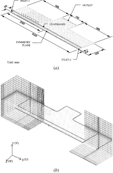
Fig. 1—Schematic of the experimental setup for spreading carbon fiber tow: (a) top view and (b) side view.
single fiber prediction showed that the results were not satis-fied because the flow field was too complicated.
⫺ ⭸⭸x j
冤
冢
⭸ui ⭸xj ⫹⭸uj ⭸xi冣
冥
⫽ 0, i, j ⫽ 1, 2, 3 None of the previous works investigated the internal flowpatterns in qualitative and quantitative analysis about the spreader. Therefore, the exact flow field of the spreader is
where ujis the velocity, p is the pressure,is the constant
still unknown. The objective of the present study is to
estab-density, andis the molecular kinematic viscosity. The ui,uj
lish a three-dimensional (3-D) mathematical model of the
are the fluctuation parts of the velocity uiand uj; and u⬘iu⬘j
spreader by operating a numerical technique of far-field
is the Reynolds stress tensor, which can be modeled by the treatment and to provide a 3-D numerical flow visualization,
eddy viscosity hypothesis: which reveals velocity fields, pressure distributions,
stream-lines, and useful flow patterns. The flow patterns contribute u⬘
iu⬘j⫽˜ij
to understanding the detail flow field in the physical model,
and then help us to develop a new efficient spreader. Finally, ⫽1 ˆij
a pneumatic spreading system is constructed. In this model system, carbon fiber sheet can be prepared from fiber tow.
Meanwhile, photography is used to record the carbon fiber ⫽2
3␦ijk⫺ 2
3Tⵜ ⭈ ui␦ij⫹T(ⵜui⫹ (ⵜui)
T)
tow spreading process. The spreading mechanism of the
carbon filaments is also investigated by combing numerical Here, k⫽ (1/2) u2is the turbulent kinetic energy, and
Tis
simulation and experimental analysis. the eddy viscosity. They have to be prescribed by a
turbu-lent model.
The generic k- model can be described as[24]
II. GOVERNING EQUATIONS AND
TURBULENCE MODEL
⭸k⭸t⫹ⵜ ⭈ (uik)⫽ ⵜ ⭈ ((⫹kT)ⵜk) ⫹˜ijⵜ ⭈ ui⫺
The incompressible and isothermal Reynolds-averaged Navier–Stokes equations are
⭸⭸t ⫹ ⵜ ⭈ (ui) ⫽ ⵜ ⭈ ((⫹T)ⵜ) ⭸uj ⭸xj ⫽ 0 ⫹ c1/k˜ijⵜ ⭈ ui⫺ c2 2 k ⭸ui ⭸t ⫹ ⭸uiui ⭸xi ⫹1⭸x⭸p j ⫹ ⭸⭸x j
冢
u⬘iu⬘j冣
whereTable I. Model Constants Employed in the Computation c1 c2 c k 1.44 1.92 0.09 1 2.9076 k⫽ k2 (c2⫺ c1)冪c where k (Von Karman constant)⫽ 0.4187
The eddy viscosity is calculated from T⫽ c
k2
(a)
wherekand⑀are the turbulent Prandtl number for k and , respectively, and c1, c2, and c are the empirical coefficients.[25]
The set of model constants employed is summarized in Table I.
III. BOUNDARY FITTED COORDINATE AND
GRID GENERATION
In fact, the geometry of a spreader is too complex to be described by using natural analytic coordinates such as cylindrical coordinates, spherical coordinates, or bipolar coordinates. In this case, the coordinate transformation must be given numerically. There is now extensive literature on the numerical generation of boundary fitted grids.[23,25] Boundary fitted coordinates extend the capabilities of finite difference methods to deal with complex geometry. The basic ideal is to use a curvilinear coordinate transformation,
(b) mapping the complex flow domain in physical space to a
simple flow domain in computational space. In other words, the Cartesian coordinate system (xi)⫽ (x,y,z) in the physical
Fig. 2—(a) A three-dimensional mathematical model of the pneumatic spreader in a isometric view. (b) A perspective of a far-field treatment by
domain is replaced by a curvilinear coordinate system (i)
multi block technique in real space (U, V, and W are the velocity
⫽ (,,) such that boundaries of the flow domain
corre-components).
spond to the surface.
The equations are discretized with respect to the computa-tional space coordinate. Boundary conditions may be
imple-mented naturally in the rectangular computational domain. computer time, only half of the geometry was simulated. In most simulation work, the boundary conditions at inlets were However, the expense of making the partial differential
equa-tions would be higher due to the nonlinear coordination used to a uniform velocity, which was quoted from measured data, or to an ambient pressure for an internal flow field. In transformation, and a great deal of memory is wasted because
of the necessity of designating a large proportion of the grid the present study, the inlet velocity was unknown. It was difficult to measure for a sudden contraction case. Therefore, as solid. The multiblock approach was used in order to
maximize computational efficiency and to save memory.[25] we considered the realistic status as the characterization of the fluid flow in the far field. Thus, the computation domain The concept of the multiblock grid is the solution domain,
which is divided into subdomains. Each subdomain has its was extended along x direction and y directions as Figure 2(b) illustrates (a perspective view).
associated subgrid, or block. In multiblock grids, data are
transferred from one block to another using a generalization The blocks were built on each side of a spreader model. Therefore, the boundary conditions at the outer surface of of the periodic boundary condition. The blocks are arranged
to overlap such that a boundary surface of one block is each block could be specified by atmospheric pressure (101,300 Pa), and the computation of the flow field was situated in the interior of another. After each iteration, the
value of variables on the boundary of the first block must executed from the external flow field to the internal flow field. The grid employed was structured and orthogonal cross a boundary surface of the second block; values of
variables on this boundary surface can be updated using curvilinear. The number of nodes and elements were 137,800 and 129,600 in the fluid domain, respectively. A grid conver-interior values from the first block.
As shown in Figure 2(a), the geometry of the 3-D spreader gence study was performed to ensure that the resolution of this mesh was adequate. Doubling the number of nodes model was defined first in a physical space (x, y, z). Because
IV. COMPUTATIONAL DETAILS u⫹⫽ ⫺(k) 1/2 u A. Boundary Conditions and Quite a bit of literature discussed and stressed the
impor-tance of specification of the inlet boundary conditions in the
y⫹⫽ ⫺(k)
1/2 (d⫺ y) computation of turbulent flows. Sturgess et. al.[26]showed
that the numerical simulations of flows were highly sensitive
The scaled velocity component parallel to the wall and to the assumptions made for inlet boundary conditions.
in the x directions is Choice of the computational grid was also important. They
concluded that overall accuracy of the simulation is deter-mined by assumed boundary conditions and choice of grid.
u⫹⫽
冦
y⫹, for y⫹⬍ y⫹0 1 klog (Ey ⫹), for y⫹⬎ y⫹ 0 Eaton and Johnston[27]cited that a backward-facing step flowis affected by inlet boundary conditions. They suggested that accurate specification for the inlet boundary conditions
where log is a natural logarithm. including mean velocity and turbulence details is essential to
The crossover point y0+between the viscous sublayer and correctly describe the downstream flow field. The boundary
the logarithmic region is the upper root of conditions employed were as follows.
(1) Symmetry plane y⫹0 ⫽ 1 klog (Ey ⫹ 0) V⫽ W ⫽ 0
The equation for the turbulence kinetic energy k is solved in the control volume immediately adjacent to the wall. From ⭸U
⭸x ⫽ 0, ⭸⭸x⫽ 0 the value of the wall shear stress, can be obtained. The turbulence dissipation is obtained from the turbulence kinetic
where energy through the relation
⫽ k, , and p
⫽ c3/4 k3/2
k(d⫺ y)
(2) Pressure boundaries
In the mathematical grid, the computational domains were extended so that the pressure boundaries could be easily
B. Discretization and Computational Procedures created and specified on the surfaces of the blocks as the
Discretization has been carried out using the finite volume inlet boundary conditions, as shown in Figure 2(b). For the
method. The governing equations were integrated over the surfaces sufficiently far downstream, fixed values of all
control volume and reduced to algebraic equations, which variables could be specified at pressure boundaries.
followed conservation laws. Once a grid of points was set
p⫽ 101,300 (Pa) (atmospheric condition) up over the field, all the unknown variables were stored in the certain of the computational cells. In order to avoid
U⫽ V ⫽ W ⫽ 0 (free stream)
pressure-velocity decoupling problems, arising from the fact
(3) Outlet that pressure and velocity were calculated in the same
loca-Static pressure was introduced at the outlet location to tion, the convection flux through each cell faces was calcu-model outflow boundary. For observing the flow field in the lated by using the modification first proposed by Rhie and 3-D spreader model, various static pressure conditions were Chow,[28] extended here for a multiblock grid. The major used for computation, including 101,100, 101,200, and achievement of this approach is that it provides a prescription 101,250 Pa, respectively. It was useful to predict the experi- for implementing the standard primitive variable algorithms mental condition and make a comparison of velocities com- such as SIMPLE and SIMPLEC using a non-staggered grid. puted by various pressure and measured data. The feature of the prescription is that the velocity needed for the calculation of the connective flux through a cell face (4) Walls
is not obtained from a linear interpolation of the adjacent The boundary wall was fixed, and a no-slip condition was
cells’ velocities. However, the velocity is modified to be imposed on all velocity components. Many variables varied
directly linked to the two adjacent pressure nodes. Following rapidly in the near wall regions of the flow, instead of using
this procedure, the SIMPLE algorithm was used as a pres-extremely fine grids in these regions; therefore, their
behav-sure-correction method,[29]in order to derive the pressure ior was specified with wall functions. The wall functions
equation from the continuity equation. were illustrated below by considering the flow in a fully
The treatment of the convection term determines the accu-developed boundary layer over a stationary wall.[24] Near
racy of the solutions of the model equations. The CCCT the wall ( y⫽ d), it was found that the wall shear stress
scheme was used for the discretization of convective fluxes. is related to the turbulence kinetic energy by
The CCCT scheme is a modification of the quadratic upwind
2⫽ c2k2 differencing scheme (QUICK), which is an upwind scheme
with third-order accuracy and can suffer from nonphysical A new quantity is defined such that overshoots in its solutions.[28]The diffusion terms were dis-cretized in space using a second-order centered difference k⫽c1/2 k
scheme. The set of linearized difference equations, after the discretization of the conservation equations, were passed to This may be used to define scaled variables
a simultaneous linear equation solver, which used an iterative was behind the inlet-1, which was 50-mm long. To simplify the computational problem, the distance from the symmetry solution method. The STONE method was available for this
purpose and was very efficient in a vector computer. In this plane to the clapboard was set at three different dimensions, 105, 70, and 25 mm. Similarly, the height of the spreader work, since the transient evolution was not of interest, the
time-stepping scheme could be optimized for faster conver- was also set at three different dimensions: 20, 10, and 5 mm. They were explored by using numerical simulation gence. Acceleration techniques such as false time-step
were applied.[25] at various boundary conditions, whereas the computational
results were useful in understanding how air fluid interacted Therefore, a typical simulation of the 3-D model on the
base mesh required 300 MB of memory, and consumed a with carbon fibers.
According to the simulate results, the spreader would be total CPU time of 7.237⫻ 104seconds. The program was
executed on a vector computer, CRAYJ916* supercomputer, modified and spread experiments would be undertaken to test the applicability of the 3-D mathematical model. First,
*CRAY J916 is a trademark of Cray Research, Inc., Minneapolis, MN.
the downstream pressures and velocities near the outlet were measured by a precision pressure controller and digital with eight 100 MHz processors and 1 GB main system RAM.
micromanometer, under various flow rates without carbon fiber tow, and the velocities were compared with the
calcu-V. EXPERIMENT lated data to confirm the accuracy. Experiments of fiber
spread were executed at various fiber transporting rates and A. Experimental Setup
air flow rates. Photography techniques were used to record Experiments were conducted using the setup shown sche- the processes of fiber spread. The photographs were taken matically in Figure 1. The main elements were comprised from the top view. Five Nikon FM2 cameras were used in a sequence of the tow feed spool, tension control device, and each was fitted with a 52-mm lens. The single-frame pneumatic tow spreader, vacuum pump, and take-up spool. photographs were taken with shutter speeds of 1/15 to 1/60 The fibers from the carbon fiber tow containing 12,000 seconds, so that the images showed how fiber was spread filaments were passed through a fiber guide into a first and moved in the pneumatic spreader.
friction roller. The first roller was synchronized with the second friction roller at a constant rate of speed. The two
VI. RESULTS AND DISCUSSION
rollers were controlled by a variable speed driver. Hence,
the fibers between the two rollers, which were subsequently To study the geometry effect of the spreader, the simula-spread in the pneumatic simula-spreader, remained in a low tensional tion was conducted using height with three different dimen-state that was given by the tension control device. For the sions, 20, 10, and 5 mm. Hence, there were three different air flow rate in the pneumatic spreader, the vacuum pump cross-sectional areas: 500 and 100 mm2at 1 and inlet-sucked air and gave a stable control of flow rate, which was 2, for case 1, respectively; 250 mm2at inlet-1 and 50 mm2 measured by a multiple tube flow meter and a precision at inlet-2 for case 2; and 125 mm2at inlet-1 and 25 mm2at pressure controller. After the fibers spread and left the second inlet-2 for case 3. The boundary conditions using pressure roller, the fibers were taken up by a take-up system. drop (0.275 psi) between upstream and downstream were given by Baucom et al. It was found the pressure dropped abruptly as the cross-sectional area decreased, which caused B. Experimental Techniques
a significant increment in air flow velocity at inlet-1 from The design of the spreader must satisfy several interacting 21.6 m/s for case 1 up to 44 m/s for case 3. The velocity requirements. Although high air velocity resulting drag force increase is inversely proportional to the cross-sectional area, to fibers is desirable, streamwise velocity is constrained by while the pressure drop is related to the square of the flow the need to avoid circulation and excessive agitation of the velocity. The pressure drop is also inversely proportional to airflow. Agitation can cause fibers to become entangled, the cross section of the fiber flow outlet (inlet-1). Hence, which makes fiber spread difficult and damages fibers. This the spreader model was set with 5 mm in height.
is the first 3-D mathematical model of a pneumatic spreader. The other parameter, the distance from the symmetry Therefore, the height of the spreader and the distance from plane to the clapboard, was also set with three dimensions the symmetry plane to the clapboard were the two design 105, 70, and 25 mm. The flow field for the distance 25 mm parameters in the spreader. The spreader formed by PAN was taken as an example shown in Figure 3. The streamlines (polyacrylonitrile) pieces, which were transparent allowing were plotted at the central plane ( y⫽ 25 mm) of the mathe-the spread procedure of carbon fibers to be photographed matical model. There were three circulations in the spreader. for subsequent qualitative comparison with computational
(1) The air was sucked into the spreader and then the air results, had a through-length 500 mm in x-direction, as
was accelerated due to sudden contraction at inlet-2. shown in Figure 2(a). The half-width of the spreader was
Therefore, the circulation zone was formed by fluid one-fourth (125 mm) of the length.
viscosity and drag. The projecting part connected to a vacuum pump had the
(2) The air flow entered inlet-1 and passed through the nine width 80 mm in the z direction and a length of 110 mm in
slots on the clapboard; thus, there were two circulation the x direction. The fiber entrance named inlet-2 was 2.5
zones behind the clapboard. mm in half-width. The fiber exit named inlet-1 had a
25-mm half-width selected as the final fiber spread width. The However, the main interest of the present investigation was the flow field from the symmetry plane to the clapboard. clapboard contained nine slots, which were parallel to the
symmetry plane. While the distance increased from 25 to 105 mm, the
circula-tion zone would increase at inlet-2 and appear at inlet-1; it Each slot was 5-mm wide and 10 mm apart; the first slot
(a)
Fig. 3—A complete view of streamlines at the central plane ( y⫽ 2.5 mm) under pressure drop 50 Pa between far-field pressure boundary and outlet pressure boundary.
(b)
Fig. 5—Pressure contour under pressure drop 50 Pa: (a) a complete view Fig. 4—Velocity-vector representation of the flow field in Fig. 3.
and (b) a close-up view.
makes fiber spread difficult. Since there was a slow velocity in the circulation zone, the fibers were hard to drag by air flow. In order to avoid the circulation zone, the distance from the symmetry plane to the clapboard was set with 25 mm. To understand the flow field under various boundary conditions, three cases with different pressure boundary con-ditions at the outlet surface were examined with the two parameters in the model. For the three cases, the pressures were 101,100, 101,200, and 101,250 Pa, respectively; how-ever, the calculated flow fields were all very similar, so only the flow field for case 3 (101,250 Pa) was shown in Figures 3 and 4.
A velocity vector showed the main characteristics of the air flow. The varieties of flow velocity appeared at inlet-1 and slots, since the cross-sectional area decreased. However, there was a stable flow downstream around the outlet. The velocity of air flow showed an extremely small difference
Fig. 6—Calculated pressure distributions at the inside and outside of the
between inlet-1 and inlet-2. It is well known that Q ⫽
inlet-1 (inside of the inlet-1: — — —, ---; inlet plane: — — —; outside
UA, where Q is the flux, is the fluid density, U is the
of the inlet-1: – –).
fluid velocity, and A is the cross-sectional area of inlet. Furthermore, the flux at inlet-1 was 10 times larger than that at inlet-2, and the slots on the clapboard were close to
inlet-1; therefore, the main variations in air flow would occur the spreader, but an evident difference was presented in case 1 (101,100 Pa). Therefore, if the simulation was in a low at inlet-1 nearby, so we concentrated the discussion in the
region from inlet-1 to the slots. speed flow field, we could remove the outward block and
take an ambient pressure boundary in the vicinity of inlet-A complete view of the pressure contour was seen in
Figure 5(a), which showed the low pressure distributed at 1 and inlet-2 to save the CPU time. In other words, the treatment of far-field boundary conditions has good calcu-the slots. A close-up view of calcu-the pressure contour in calcu-the
vicinity of inlet-1 was shown in Figure 5(b). The detail lated results at high speed flow field. Figure 6 showed that the calculated pressure distributions were at the inside and pressure distribution was calculated and had a slight
Fig. 7—Calculated W-velocity components from symmetry plane to the Fig. 9—Calculated U-velocity components from symmetry plane to the clapboard along x-direction in the vicinity of inlet-1 (inside of the inlet- clapboard along x-direction in the vicinity of inlet-1.
1:---, – –; inlet plane: — — —; outside of the inlet-1: — — —, ---, – –).
Fig. 10—Calculated U-velocity distributions from symmetry plane to the clapboard in front of slots 1, 5, and 9.
Fig. 8—Calculated W-velocity distributions from symmetry plane to the clapboard in front of slots 1, 5, and 9.
at the inlet of a fluid; therefore, the numerical error could not be avoidable.
abruptly due to a sudden contraction. There was some
differ-ence about 20 Pa between the inside and outside of inlet-1. The W-velocity component at slots 1, 5, and 9 was calcu-lated and presented in Figure 8. Each curve represented the Additionally, a narrow low pressure zone (z ⫽ 0.022 to
0.025 m) formed near the clapboard because the air flow velocity variation of each slot from the symmetry plane. The physical model was constructed according to the passed through the separation location S; hence, air flow
separation generated. Air could not enter this zone near the designed parameters. To test the accuracy of the numerical experiment, a series of experimental measurements were clapboard, so it was thin and there was no air flow; thus,
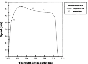
pressure dropped. made, and a comparison of the calculated velocity with the
measurement is presented in the following figures. Figure The distribution of the lateral velocity W was reducing
with the distance Z approaching the symmetry plane. 12 shows a comparison between computation and measure-ment of the outlet velocity at the static pressure on the Inversely, the more air flowed into the inner location, the
more velocity W increased. Above all, much variation in the centerline of the outlet. It was found that the computational data were in good agreement with the measured data. Similar velocity W existed behind the slots. The calculated velocity
W in the vicinity of inlet-1 was shown in Figure 7. There trends were observed at the static pressure, 101,200 Pa, as shown in Figure 13.
was a larger velocity at the outside of inlet-1 near the
clap-board, while the air was sucked into the spreader. It should Theoretically speaking, the converged solution was calcu-lated from upstream to downstream; moreover, the upstream be noted that the treatment of far-field boundary could
facili-tate the calculation at the cross section of inlet-1. Generally, computational results had the same order in numerical error as the downstream. The simulated and measured data were the calculation of the internal flow field set a uniform inflow
both qualitatively and quantitatively similar; further, the 3-D computational results can be helpful for designing a pneu-matic spreader. Although considering no fiber addition might not be precise enough to lead to an understanding of the interaction of fiber and air flow, the results gave us insight and led to the realization of the 3-D flow field.
The air flux was related to the fluid velocity and pressure in the spreader and was controlled by the flowmeter. They were measured and presented in Figures 14(a) and (b). It was found that the mean mass flow rate was proportional to the mean static pressure and mean static pressure was also linearly increased with mean fluid speed. Similarly, the computational results have the same trend as the measured results. Therefore, the flow field can qualitatively be under-stood before the fiber spreading experiment is executed.
Figure 15 shows a fiber spreading experiment under
VF ⫽ 7 m/min and Q ⫽ 90 L/min, perpendicular to the
Fig. 11—Calculated speed distributions from symmetry plane to the clap- center of a slot. It was seen that air flowed toward the slots, board in front of slots 1, 5, and 9. yielding a slight change in velocity, but the magnitude of
the velocity increased abruptly near the slots (Z⫽ ⫺0.02 m), since the cross-sectional area was suddenly contracted. The air entered the spreader through inlet-2 and turned toward slot 9; therefore, the W velocity at slot 9 is larger than that at other slots. The air flow was accelerated at the inside of inlet-1 and inlet-2, and the large velocity U was near the symmetry plane. The U-velocity gradually decayed at the inner location, while the air flow turned toward slots on the clapboard (-Z direction).
Figure 9 presented the calculated U-velocity in the vicinity of inlet-1. The U-velocity with an average velocity 0.6 m/s at the outside of inlet-1 (x⫽ ⫺260 mm) was accelerated up to an average velocity 5.5 m/s at the inside of inlet-1 (x⫽ ⫺248 mm). Moreover, as has been realized by previous discussion, the air flow could not enter the low pressure zone near the clapboard (Z ⫽ ⫺0.22 m) due to the effect of separation flow. Hence, little air flowed in this zone, so that the U-velocity decayed. The distribution of the U-veloc-ity component from the symmetry plane to the slots was shown in Figure 10. The results indicated that there were
Fig. 12—Comparison of computational and measured speed at outlet under
pressure drop 50 Pa. smaller U-velocity components at the inner location due to the air flow turned direction. There was a negative U-velocity around slot 9; this was because air flow came from inlet-2. In this investigation, because the V-velocity component was not found, it was found that the flow field was a two-dimensional flow in the spreader.
Figure 11 showed the speed variations in front of slots 1, 5, and 9. The speed was the resultant velocity of U- and W-velocity components. The results indicated that the main air flow come from inlet-1 and there was similar magnitude of speed around where VFwas the fiber transporting velocity
and Q was the air mass flow rate. It was seen that the fibers were easily spread, and most fibers were dragged toward the clapboard and concentrated at the clapboard side; the reason for this was that the fluid velocity was fast.
While the conditions were set with VF ⫽ 7 m/min and Q⫽ 70 L/min, the fibers were spread in width about 20
mm at fiber exit. Fiber tow was spread by axial velocity; however, the axial velocity was not large enough to make fibers move to the location where the lateral W-velocity was larger. However, Baucom et al. argued that air entered
Fig. 13—Comparison of computational and measured speed at outlet under
(a) (b)
Fig. 14—(a) The relations of the experimentally measured mean mass flow rates and pressure drops at outlet. (b) The relations of the experimentally measured pressure drops and speeds at outlets.
Fig. 15—Photograph of fibers spread experiment under VF⫽ 7 m/min and Q ⫽ 90 L/min.
the clapboard of the expansion section into a vacuum mani- reported that the 12 k tow was spread to a 5.08-cm width at a tow rate of VF⫽ 3 m/min, and the pressure drop was
fold. This cross-flow of air provided drag on the carbon
fibers, resulting in tow spread across the pneumatic spreader. kept at P ⫽ 0.275 psi.
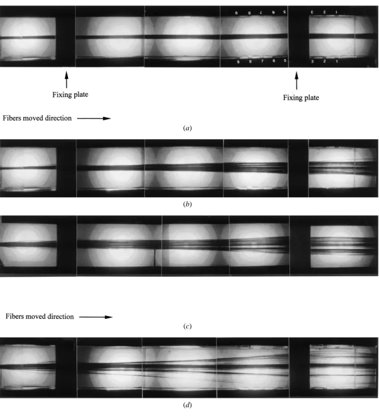
In this study, we proposed an excellent performance and The fiber spread procedure at the condition VF ⫽
7 m/min and Q⫽ 80 L/min was shown as follows. Figure efficiency application for spreading a fiber tow. Additionally, in a continuous fiber spreading procedure, there were three 16(a) indicates that the fiber tow was transported in the
spreader. Initially, the fiber tow was spread out and fluffy main steps recounted as follows: at the fiber exit, as shown in Figure 16(b), because there
(1) the fiber flow was first spread at the fiber exit by the was a maximum axial U-velocity at the exit (inlet-1) due
axial air flow; to a sudden contraction and an acceleration of air flow.
(2) fibers gradually moved toward the lateral side, and the Sequentially, fibers were gradually spread out, and the partial
lateral W-velocity influenced the fiber movement; and spread fiber extended to the inner of the spreader about
(3) the fibers were closer to the clapboard; as the W-velocity the location of the fifth slot, as shown in Figure 16(c).
increased, the fibers were dragged toward the clapboard. Futhermore, the spread width at the inner location was
slightly larger than that at the fiber exit, because the air flow The proposed spread procedure was more detailed and quite different from that of Baucom et al. Indeed, the 3-D computa-turned toward the slots. Compared to Figure 8, the air drag
was gradually increased. Finally, fibers were dragged toward tional results can be helpful for designing a pneumatic spreader. Resigning a pneumatic spreader intends to satisfy the clapboard and maintained the width they had when they
left the spreader, as shown in Figure 16(d). There were various requirements, such as stable flow field, avoiding circulation and vortex, and no abrupt velocity and pressure similar spread results on the other conditions, and the fiber
(a)
(b)
(c)
(d)
Fig. 16—Photographs of fibers spread experiment under VF⫽ 7 m/min and Q ⫽ 80 L/min: (a) initial state, (b) fibers spread to lateral side, (c) more fibers
moved to lateral side, and (d ) final state.
Although our simplified simulation without fiber tow may VII. CONCLUSION
not be precise enough, the results give us a detailed
quantita-This is the first 3-D mathematical model of the fiber tive observation to explore the 3-D flow field, i.e., velocity
spreader and the first time it has been viewed using a photo-and pressure distribution. The comparison between the
graphic technique. The major results and conclusion from simulated and experimental results clearly shows that the this work are summarized as follows.
numerical approach reported here can be used to study the
multiblock technique, which extends the computational turbulent Prandtl number for
shear stress
domain to far upstream, can improve the calculated
accu-racy at the fiber exit (inlet-1) nearby, and it is more useful ˜ij Reynolds stress tensor
general variable
at large pressure drop conditions.
2. The turbulent k- model, which includes incorporation Mathematical Operators of a wall function, is employed to study the fluid behavior 䉮 del operation of air flowing through the spreader. The circulation zone ⭸ partial derivative and separation flow can be simulated accurately.
3. The simulation results are in excellent agreement with
REFERENCES the experimental measurements downstream, and the
1. F. Delannay, L. Foryen, and A. Deruyttere: J. Mater. Sci., 1987, vol.
result can be used to analyze the flow field upstream.
22, pp. 1-16.
Therefore, the designed parameters are determined; the
2. R.V. Subramanian and A. Nyberg: J. Mater. Res., 1992, vol. 7 (3),
height of the spreader is 5 mm, and the distance from pp. 677-88.
clapboard to symmetric plane is 25 mm. 3. Li-Min Zhou, Yiu-Wing-Mai, and Caroline Baillie: J. Mater. Sci., 1994, vol. 29, pp. 5541-50.
4. The fiber tow was successfully spread at various
condi-4. Sunil G. Warrier and Ray Y. Lin: Scripta Metall. Mater., 1993, vol.
tions, and the performance is better than in prior studies.
29, pp. 1513-18.
The optimum and efficient condition in the fiber spread- 5. Zhenhia Xia, Yaohe Zhou, Zhiying Mao, and Baolu Shang: Metall. ing operation is VF⫽ 7 m/min and Q ⫽ 80 L/min, and Trans. B, 1992, vol. 23B, pp. 295-302.
6. R. Asthana: J. Mater. Sci., 1998, vol. 33, pp. 1959-80.
the operating pressure drop is 33 Pa, which is smaller
7. G. Leonhardt, E. Kieselstein, H. Podlesak, E. Than, and A. Hofman:
than Baucom and Marchello reported.
Mater. Sci. Eng., 1991, vol. A135, pp. 157-60. 5. The fiber spreading procedures are first proposed, and
8. Andreas Mortensen: Mater. Sci. Eng., 1991, vol. A135, pp. 1-11.
they can help in understanding the spread process and 9. J.K. Yu, H.L. Li, and B.L. Shang: J. Mater. Sci., 1994, vol. 29, pp. provide the ability to test the design of the pneumatic 2641-47.
10. D. Huda, M.A. El Baradie, and M.S.J. Hashmi: J. Mater. Processing
spreader.
Technol., 1993, vol. 37, pp. 529-41. 6. The 3-D simulation is successfully combined with
experi-11. Feng Wu and Jing Zhu: Composites Sci. Technol., 1997, vol. 57, pp.
ment for the application of carbon fiber tow spread, and 661-67.
this methodology is often used in the fiber spread process. 12. Susan Abraham, B.C. Pai, K.G. Satyanarayana, and V.K. Vaidyan: J.
Mater. Sci., 1999, vol. 25, pp. 2839-45.
13. S. Abraham, B.C. Pai, and K.G. Satyanaryana: J. Mater. Sci., 1992, vol. 27, pp. 3479-86.
14. H.M. Cheng, A. Kitahara, S. Akiyama, K. Kobayashi, and B.L. Zhou:
NOMENCLATURE
J. Mater. Sci., 1992, vol. 27, pp. 3617-23.
A cross-sectional area 15. Yu-Qing Wang and Ben-Liam Zhou: J. Mater. Processing Technol.,
1998, vol. 73, pp. 78-81. c1, c2, empirical coefficient
16. R.J. Bobka and L.P. Lowell: Handbook of Composites, vol. 1 - Strong
and c1 Fibres, W. Watt, and B. V. Perov, eds., Elsevier Science Publisher
E empirical coefficient B.V., 1985, pp. 579-80.
k turbulent kinetic energy 17. D. Clark, N.J. Wadsworth, and W. Watt: Handbook of Composites,
vol. 1 - Strong Fibres, W. Watt, and B. V. Perov, eds., Elsevier Science
p pressure
Publisher B.V., 1985, pp. 579-80.
t time
18. Haining Yang, Mingyuan Gu, Weiji Jiang, and Guoding Zhang: J.
u⬘iu⬘j Reynolds stress tensor Mater. Sci., 1996, vol. 31, pp. 1903-07.
u⬘i, u⬘j fluctuation parts of the velocity 19. Clare G. Daniels: U.S. Patent No. 3,873,389, Philco-Ford Corp.,
Phila-uj velocity delphia, PA, El Toro, CA, Mar. 25, 1975.
20. Paul E. McMahon, Tai-Shung Chung, and Lincoln Ying: U.S. Patent
u average velocity
No. 4,871,491, BASF Structural Materials, Inc., Charlotte, N.C., Oct.
u+ scaled velocity
3, 1989.
U, V, W velocity components 21. John N. Hall: U.S. Patent No. 3,704,485, Hercules Incorporated,
Wil-VF fiber transported velocity mington, DE, Brookside Park, DE, Dec. 5, 1972.
22. Robert M. Baucom and Joseph M. Marchello: Sampe Q., 1990, July, x, y, z Cartesian coordinates
pp. 14-19.
y+ dimensionless distance
23. J.F. Tompson: Numerical Grid Generation, Elsevier, New York, NY, 1982.
Greek Characters
24. E.B. Launder and B.D. Spalding: Mathematical Models of Turbulence,
turbulent dissipation rate
Academic Press, London, 1972.
turbulent viscosity 25. CFX-F3D Version 4.1 User Manual, Harwell Laboratory, Oxfordshire,
k Von Karman constant U.K., 1995, Oct.
26. G.J. Sturgess, S.A. Sayed, and K.R. McManus: Int. J. Turbo Jet ,, curvilinear coordinate
Engines, 1986, vol. 33, pp. 43-55.
v molecular kinematic viscosity
27. J.K. Eaton and J.P. Johnston: AIAA J., 1981, vol. 19 (9), pp. 1093-1100.
vT eddy viscosity 28. M.C. Rhie and L.W. Chow: AIAA J., 1983, vol. 21, pp. 1525-32.
density 29. S.V. Patankar and B.D. Spalding: Int. J. Heat Mass Transfer, 1972,
vol. 15, pp. 1787-92. K turbulent Prandtl number for k