開發具非等效平行機之彈性流程式生產的啟發式排程方法

行政院國家科學委員會專題研究計畫 成果報告

開發具非等效平行機之彈性流程式生產的啟發式排程方法

研究成果報告(精簡版)

計 畫 類 別 ： 個別型 計 畫 編 號 ： NSC 95-2221-E-004-006- 執 行 期 間 ： 95 年 08 月 01 日至 96 年 07 月 31 日 執 行 單 位 ： 國立政治大學資訊管理學系 計 畫 主 持 人 ： 陳春龍 計畫參與人員： 博士班研究生-兼任助理：陳俊龍 處 理 方 式 ： 本計畫可公開查詢

中 華 民 國 96 年 11 月 12 日

(This paper has been accepted for publication by International Journal of Production Research)

Bottleneck-based heuristics to minimize tardy jobs in a flexible flow line with unrelated parallel machines

CHUN-LUNG CHEN and CHUEN-LUNG CHEN*

*_{Department of MIS, National Chengchi University, ZhiNan Rd., Wenshan District,} Taipei City 11605, Taiwan, R.O.C.

1. Proposed bottleneck-based heuristics

Lenstra et al. (1977) proved that the FFL with two stages is NP-hard in the strong sense, so the candidate problem is a NP-hard problem as well. It requires much computational time to find the optimal solution. A heuristic is an acceptable practice to find a good solution. In this paper, several bottleneck-based heuristics are proposed to solve the candidate problem with unrelated parallel machines. The heuristics consist of three steps:

Step 1. Identify the bottleneck stage.

Step 2. Schedule jobs at the bottleneck stage and the upstream stages. Step 3. Schedule jobs at the downstream stages

The workload is used as an indicator to identify the bottleneck stage. Since the machines are unrelated at each stage, the processing time of an operation at a stage is dependent upon the machine assigned to the operation. The workload of stage j is computed by the sum of the average processing times of all the operations processed at the stage divided by its number of machines, denoted as Rj= j

n

i p /ij) m

( 1

∑

= . The stage with the largest Rj, is defined as the

bottleneck stage.

When scheduling jobs at the bottleneck stage, the arrival times of the jobs to the bottleneck stage must be determined. Since the bottleneck stage may not be the first stage, the arrival times of the jobs to the bottleneck stage may not be zero. The sum of the processing times of the operations at the upstream stages of a job is commonly used as the arrival time to the bottleneck stage of the job (Lee et al. 2004). However, since it will produce infeasible schedule, complicated procedures are needed to modify the schedule at the bottleneck stage until a feasible and promising schedule is obtained. This method of determining a job’s arrival time to the bottleneck stage will be even more difficult for the candidate problem because the processing time of an operation at a stage is not a constant in an unrelated parallel machines environment.

In this research, we propose a new approach to iteratively schedule the jobs at the bottleneck stage and the upstream stages. At the initial iteration, let all the jobs be unscheduled jobs; for each unscheduled job, three machine selection rules are used to assign the job to a machine at each of the upstream stages and determine the arrival time of the job to the bottleneck stage. When the arrival times of all the unscheduled jobs to the bottleneck stage are determined, two decision rules are used to select the best job for the bottleneck stage. The schedule of the selected job at the upstream stages and the bottleneck stage is then fixed. This job becomes a scheduled job, and the next iteration follows to schedule the remaining unscheduled jobs under the constraint of the scheduled jobs. This procedure will continue until all the jobs are scheduled. Since, in each iteration, the new approach constructs the schedule at each of the upstream stages and the bottleneck stage by adding only one job to the schedule of the stages constructed in the previous iteration, it clearly will produce feasible schedules. This procedure neatly overcomes the difficulty of determining feasible arrival time of a job at the bottleneck stage, especially when unrelated parallel machines are

considered. When the arrival times of all the jobs at the bottleneck stage are determined, any heuristics for unrelated parallel machines can be applied to schedule the jobs at the bottleneck stage.

The three machine selection rules used in this research are as follows: given a job at a stage, the first machine selection rule, EAAM, is to select the machine with the earliest available time among the available machines. The second selection rule, ECAM, is to select the machine with the earliest completion time when the job is assigned to the available machines. The third selection rule, ECALLM, is to select the machine with the earliest completion time when the job is assigned to all the machines at the stage, including available and unavailable machines. This rule may cause an idle period of the job. However, since unrelated parallel machines are considered at the stage, an unavailable but more efficient machine may produce earlier completion time for the job. When the machine selection rules are used in the bottleneck-based heuristics to determine the arrival time of a job to the bottleneck stage, the application is straightforward. Since only one job is considered at a time, when the job arrives at each of the upstream stages, it is easy to calculate its completion time on each available machine and each unavailable machine and determine the machine that the job will be assigned to according to the machine selection rules. However, when the machine selection rules are applied with dispatching rules, the procedure will become more complicated. Since the candidate problem is a flow shop problem, we can schedule jobs stage by stage. At each stage, an array is set to record the updated machine available time for each machine, and an array is set to record the updated arrival time of each job. Also, a time clock is set to record the updated decision time for schedule making; the updated decision time is the smallest updated machine available time. The initial available times of all the machines are zero, and the initial arrival time of a job is its completion time at the previous stage. When the time clock runs to time t, the machine or machines whose updated available time(s) are earlier than time t will be identified, and the job or jobs whose updated arrival times are earlier than time t will be identified. Then, the dispatching rules will be used to select the best available job, the machine selection rules will be used to assign an appropriate machine to the selected job, and the completion time of the job on the machine will be used to update the available time of the machine.

The two decision rules at the bottleneck stage are derived by considering a variation of Moore’s algorithm (Moore 1968), which minimizes the total number of tardy jobs for single machine scheduling. The main idea of Moore’s algorithm is that it does not consider a job for scheduling if the job is decided to be tardy. As for the non-tardy jobs, they are scheduled according to the earliest due date (EDD) rule. The decision rules compare a job’s due date and completion time to justify its tardiness. Two types of due dates and two types of completion times are considered. Given a job, say job i, the two types of due dates are the given due date (di) and the estimated operational due date (d)_i=d_i −w_ibmin), and the two types

of completion times are the completion time at the bottleneck stage b (C =_ib min{ _{ibs ibs}}

s R + p )

and the estimated completion time at the last stage J (C)_iJ= min

ib ib w

C + ). Note that Ribs is the

ready time of job i to be processed on machine s at the bottleneck stage, which is the larger value between the arrival time of job i at the bottleneck stage and the available time of machine s at the bottleneck stage. Also, since unrelated parallel machines exist at the bottleneck stage, job i can be assigned to any machine s at the stage. Its completion time (C ) is defined to be the smallest of the completion times on all the machines at the stage _ib

(min{ _{ibs ibs}}

s R + p ). When the tardiness of all the jobs is justified, the non-tardy jobs will be

smallest due date, min{d_iC)_iJ ≤d_i}. The second decision rule selects the job with the smallest estimated operational due date, min{ min min}

ib i ib ib i w C d w d − ≤ − . If there are no

non-tardy jobs present, the job with the minimum completion time at the bottleneck stage will be chosen.

The decision rules using the minimum remaining processing time of job i after the bottleneck stage b, min

ib

w , in d)_i and C)_iJ was based on a thorough experiment. Since there

are unrelated parallel machines in the stages, a job’s remaining processing time after the bottleneck stage (the downstream stages) is not a constant. We defined the remaining processing time in three ways: the minimum, the average, and the maximum. The minimum remaining processing time of a job was to sum up the minimum processing time of the job on every one of the downstream stages. Similarly, the average and maximum remaining processing times were found the same way as the minimum remaining processing time. A large number of test problems were developed to evaluate the performance of the decision rules with minimum, average, and maximum remaining processing times. In terms of the average number of tardy jobs, computational results showed that the rules with minimum remaining processing time performed slightly better than the rules with average remaining processing time, and it significantly dominated the rules with maximum remaining processing time. Therefore, decision rules with minimum remaining processing time were chosen in this research.

The procedures, up to the bottleneck stage, of the proposed bottleneck-based heuristics are presented with respect to each of the decision rules:

Procedure 1: Bottleneck with due date (BDD)

Step 1. Assign all the jobs to set Ω, where Ω = {1, 2, 3, …, n}. Set the schedule for the

bottleneck stage S = φ.

Step 2. If Ω is φ, then stop.

Step 3. Compute the arrival time for each job i∈Ω at the bottleneck stage b (a ). _ib

Step 4. Compute the completion time for each job i∈Ω at the bottleneck stage b (C ). _ib

Note that C = _ib min{ _{ibs ibs}}

s R +p .

Step 5. Compute the estimated completion time C)_iJ, where C)_iJ= min

ib ib w

C + for each job

Ω ∈

i .

Step 6. Let U = {i|C)_iJ ≤d_i} and V = {i|C)_iJ >d_i}.

Step 7. If U≠φ, select the job with the smallest due date. If there are more than one job with the same smallest due date, select the one with the smallest estimated completion time, C)_iJ. If U = φ, select the job with the smallest value of C _ib

for i∈V. Let the selected job be job k.

Step 8. Save the schedule of job k at the bottleneck stage to schedule S and remove k from

Ω. Fix the schedule of job k at the upstream stages and the bottleneck stage.

Step 9. Go to step 2.

Procedure 2 is identical to Procedure 1 except for Step 5 to Step 7 to implement different decision rules.

Procedure 2: Bottleneck with estimated operational due date (BODD)

Step 5. Compute the estimated operational due date, d)_i, whered)_i= min

ib i w

d − , for each job

Ω ∈

Step 6. Let U = { min} ib i ib d w C i ≤ − and V = { min} ib i ib d w C i > − .

Step 7. If U≠φ, select the job with smallest estimated operational due date. If there are more than one job with the same smallest estimated operational due date, select the one with the smallest completion time at the bottleneck stage, C . If U = _ib φ, select the job with the smallest completion time at the bottleneck stage,C for _ib i∈V. Let the selected job be job k.

When the jobs for the bottleneck stage and the upstream stages are scheduled, the jobs will move to the downstream stages according to their schedule at the bottleneck stage, that is the schedule S, and the dispatching rules will be used to schedule the jobs at the downstream stages. Many dispatching rules have been developed for flexible flow line problems. Hunsucker and Shah (1992) evaluated the performance of six priority rules under congestion levels in the constrained flow shop with multiple processors for mean tardiness and number of tardy jobs. This study suggested that the SPT rule yielded good performances for both the performance measures considered. Brah (1996) examined the performance of ten well-known dispatching rules in static flow shop with multiple processors. The study suggested that S/RPT+SPT, MDD, and EDD rules would be best for mean tardiness and maximum tardiness. Kadipasaoglu et al. (1997) conducted a study to make a comparison of dispatching rules in static and dynamic hybrid flow systems. The COVERT rule performed well in regards to the total tardiness criterion in their research. Jayamohan and Rajendran (2000) studied many dispatching rules in flexible flow shops. They reported that simple dispatching rules, such as SPT, could offer a good performance for the number of tardy jobs. Lee et al. (2004) used several dispatching rules to compare the performance with their proposed heuristics in the hybrid flow shop. The ATC and COVERT dispatching rules showed good results in regard to the total tardiness. Since the previous researches showed different conclusions regarding the performance of the dispatching rules on the FFL problems with due date related objectives, a pilot experiment with a large number of randomly generated problems was conducted to evaluate the effect of all the previous dispatching rules on scheduling the jobs at the downstream stages in the proposed bottleneck-based heuristics. Computational results showed that these dispatching rules have insignificant effect on the proposed heuristics; however, ATC performed slightly better than the other dispatching rules. Therefore, ATC was chosen to schedule the jobs at the downstream stages, and two bottleneck-based heuristics, denoted as BDD+ATC and BODD+ATC, were developed for the candidate problem. Priority functions of the six dispatching rules are stated as below:

(1) Shortest Processing Time (SPT)

ij i p

Z =

(2) Earliest Due Date (EDD)

i i d

Z =

(3) Modified Due Date (MDD) }

,

max{ _{i i}

i d t w

Z = +

(4) Combining of the Slack per Remaining Work and the Shortest Processing Time (S/RPT + SPT) } , / ) max{( _{i i i ij ij} i d w t w p p Z = − − ×

(5) Apparent Tardiness Cost (ATC)

ij ij ij i i i d c w p p t a p p Z =−exp[−{ − ( − )− − }+/ ⋅ ]/

(6) Cost Over Time (COVERT) + + _{⋅ ⋅} − − − − = [{1 ( _{i i} ) / _i}/ _ij] i d w t a c w p Z 2. Computational experiments

In order to evaluate the performance of the bottleneck-based heuristics, a series of computational experiments have been conducted to compare the results produced by the heuristics and the dispatching rules on randomly generated problems under different production scenarios. Table 1 summarizes the experimental factors used to define the production scenarios: the number of jobs, the number of stages, the variation of job processing time, the tightness of job due date, the position of the bottleneck stage in the flow line, and the workload difference between bottleneck and non-bottleneck stages. The number of jobs has three levels with values set at 30, 50, and 100 (low, medium, and high). The number of stages has three levels with values set at 5, 10, and 20 (low, medium, and high), where the number of machines at each stage is generated from discrete uniform distribution in the range of [1, 5]. The processing times of an operation on different machines at stage j are generated from a discrete uniform distribution multiplied by the number of machines at stage j,

mj. The purpose of the term, mj, is to balance the workload of the stages (Lee et al., 2004).

Three ranges are considered for the uniform distribution to define the variation of job processing time. They are the following: [10,50], [10,100], and [10,200] (low, medium, and high). The due dates of jobs are generated from a discrete uniform distribution U[L(1-T-R/2),

L(1-T+R/2)] where L is a lower bound of the makespan, and T and R are the tardiness factor

and due date range, respectively. The maximum of the total processing times of all the jobs,

∑

=

J j ij

i p

Max{ ₁ }, is a lower bound for the FFL problem with identical parallel machines (Santos et al. 1995). Since unrelated parallel machines are considered in this research, we define L to be equal to Maxi{

∑

J_j=1p_ij}. Not that this L cannot guarantee to produce the

lower bound for the candidate problem. There are three groups of T and R, [0.1, 1.6], [0.3, 1.2] and [0.5, 0.8], considered in this research. The three discrete uniform distributions for due date generation are then created as follows: U[0.1L, 1.7L], U[0.1L, 1.3L], and U[0.1L, 0.9L]. Clearly, a smaller tardiness factor, T, and a larger due date range, R, will crate a uniform distribution with wider range for due date generation, and vice versa.

The position of the bottleneck stage in the system has three levels: the first quarter, the second quarter, and the third quarter of the flow line. The exact position of the bottleneck stage is randomly selected from the first quarter, the second quarter, or the third quarter of the flow line. The workload difference between the bottleneck stage and the highest workload non-bottleneck stage is set at three ratios of 1.1, 1.5 and 2.0 (low, medium, and high). The workload of a specified bottleneck stage is created as follows: (1) with a given combination of the number of jobs and the number of stages, randomly generate the processing times of the operations of every job on every stage; (2) calculate workload Rj = j

n

i p /ij) m

(

∑

₌₁ for every stage 1 ≦ j ≦ J, and choose the stage, say stage k, with the largest R value; (3) randomly select a bottleneck stage b, b ≠ k, from a predetermined quarter on the flow line; (4) with a specified workload difference (wd), modify the processing time of job i on machine m at the bottleneck stage b, p , where new _ibm p = (old_ibm p )×(R_ibm k/old Rb)×(wd). This procedure will

guarantee that the ((new Rb)/Rk) equals the specified wd. With the six three-level factors

considered, there are a total of 729 production scenarios, and ten test problems are generated for each scenario in the experiment.

Table 2 presents the computational results of the six dispatching rules and the two bottleneck-based heuristics, with each of the three machine selection rules, for the 7290 test

problems. The average number of tardy jobs, the relative deviation index (RDI) and the number of best solutions produced (NBS) are the three criteria used to evaluate the performance of the dispatching rules and the bottleneck-based heuristics. The relative deviation index (RDI) has been used in several papers such as Lee et al. (2004) and Choi et al. (2005), which is defined as below:

RDI ⎪⎩ ⎪ ⎨ ⎧ _{− ≠} − − = otherwise. 0 0, ) ( if _{w b} b w b a _{S S} S S S S

Sa is the solution value obtained by method a, and Sb and Sw are, respectively, the best and

the worst solution values among the solutions obtained by all the methods included in the comparison.

“Please Insert Table 2 about here”

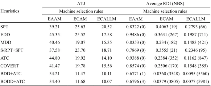
The results of the average number of tardy jobs in Table 2 show several noteworthy points. First, the machine selection rules significantly affect the performance of the dispatching rules and the bottleneck-based heuristics. When the dispatching rules are used, the average of the average number of tardy jobs produced by EAAM is 41.48; this number of ECAM and ECALLM is 22.27 and 16.97, respectively. These numbers show that ECALLM dominates EAAM and ECAM by 59% and 24%, respectively. A similar result can be obtained for the bottleneck-based heuristics; ECALLM dominates EAAM and ECAM by about 66% and 13%, respectively. Therefore, we conclude that ECALLM is the machine selection rule that should be considered for the candidate problem. Second, within each of the machine selection rules, the bottleneck-based heuristics significantly outperform the dispatching rules. When EAAM is used, the average number of tardy jobs produced by the worst bottleneck-based heuristic, BODD+ATC, is 34.40, and produced by the best dispatching rule, S/RPT+SPT, is 37.58; BODD+ATC dominates S/RPT+SPT by 8%. This dominance percentage increases to 38% and 27%, respectively, when ECAM and ECALLM are used. Also, within each of the machine selection rules, the average numbers of tardy jobs produced by the bottleneck-based heuristics are very close. These numbers are all around 34, 11, and 10, respectively, when EAAM, ECAM, and ECALLM are used. These results reach to one conclusion: the performance of the two decision rules used to schedule the jobs at the bottleneck stage is very close.

The results of the average RDI and the NBS in Table 2 strongly support the previous conclusions. For the dispatching rules, when EAAM is used, the average RDIs are all around 0.80 to 0.90. They decrease to around 0.20 to 0.40 when ECAM is used and further decrease to around 0.10 to 0.20 when ECALLM is used. On the contrary, when EAAM is used, all the NBS are 0, and they increase to a few hundred when ECAM and ECALLM are used. As for the bottleneck-based heuristics, when EAAM is used, the average RDIs are all around 0.68. They significantly decrease to about 0.04 when ECAM is used and further decrease to about 0.01 when ECALLM is used. The NBS shows the same tendency as that of the dispatching rules. When EAAM is used, all the NBS are less than or equal to 3. They significantly increase to over 3,500 when ECAM is used and further increase to over 5,500 when ECALLM is used. Therefore, we can conclude that ECALLM significantly dominates ECAM and EAAM for the dispatching rules and the bottleneck-based heuristics. Also, within each of the machine selection rules we can easily identify that the bottleneck-based heuristics significantly dominates the dispatching rules. When EAAM is used, the average RDIs of the dispatching rules are all around 0.80, and they decrease to around 0.68 when the heuristics are used. When ECAM and ECALLM are used, this comparison is even clearer; the average RDI of the dispatching rules is about 10 times that of the heuristics, and the NBS of the dispatching rules is about 1/10 that of the heuristics.

We further applied the analysis of variance (ANOVA) and Duncan's multiple range test to analyze the output (the number of tardy jobs) of the 7290 test problems to confirm the previous conclusions. The dispatching rules and the bottleneck-based heuristics are grouped into a factor and denoted as the algorithms. Table 3, the ANOVA table, shows that machine selection rules significantly affect the output of the test problems, and Table 4, the result of the Duncan test, shows that ECALLM significantly dominates ECAM and EAAM. Note that in Table 4, the machine selection rules are sequenced in descending order in terms of their average number of tardy jobs, and the rules with the same letter represent that the performance of the rules is not significantly different. Then, within each of the machine selection rules, we applied the analysis of variance and Duncan's multiple range test to test if the bottleneck-based heuristics significantly outperform the dispatching rules. Since the test results for the three machine selection rules are about the same, we present only the results for ECALLM here. Table 5, the ANOVA table, shows that the algorithms significantly affect the output, and Table 6, the result of the Duncan test, shows that the bottleneck-based heuristics significantly dominate the dispatching rules, but the performance of the heuristics is not significantly different.

“Please Insert Table 3 about here” “Please Insert Table 4 about here” “Please Insert Table 5 about here” “Please Insert Table 6 about here”

According to the previous analyses, ECALLM should be the machine selection rule chosen to work with the bottleneck-based heuristics for the candidate problem. Although the performance of the bottleneck-based heuristics is very close when ECALLM is used, all the three criteria in Table 2 show that BODD+ATC is slightly better than the other heuristics. Therefore, it is concluded that BODD+ATC working with ECALLM is the best heuristic for the candidate problem, and it is denoted as BODD+ATC/ECALLM. We further study the performance of BODD+ATC/ECALLM under different production scenarios. Table 7 summarizes the average RDI for each level of the six experimental factors for generating the 729 production scenarios. The first two factors, the number of jobs and the number of stages, are in relation to the problem size of the test problems. For each of these two factors, the average RDI values of the three levels are all within 0.007 to 0.009, so we conclude that the relative performance of BODD+ATC/ECALLM is quite robust to the problem size. The next two factors are the variation of job processing time and the tightness of job due date. Note that three different ranges are used in discrete uniform distribution to generate job's processing times. The average RDIs of the three ranges are within 0.0074 to 0.0086, so we conclude that the relative performance of BODD+ATC/ECALLM is insensitive to the variation of job processing time. As for the range of the distribution for due date generation, the low level stands for the tight range, and the high level stands for the loose range. The average RDI increases to 0.0112 when the due date range is tight (the low level). We calculated the average RDI and NBS of all the bottleneck-based heuristics and the dispatching rules at each level and found that when the due date range is getting tighter, the NBS of BODD+ATC/ECALLM decreases and causes the increase of its average RDI. However, this is the phenomenon for all the heuristics and the dispatching rules. The relative performance of dispatching rules gets even worse when due date range gets tighter. When the range is tight, the average RDI of the best-performance dispatching rule, ATC/ECALLM, is 0.1726.

The last two factors, the workload difference and the position of the bottleneck stage, are in relation to the bottleneck stage. The average RDI of the workload difference shows that the relative performance of BODD+ATC/ECALLM improves when the workload difference

increases. The average RDI decreases from 0.0099 to 0.0060when the workload difference increases from 1.1 (low level) to 2.0 (high level). This result shows that BODD+ATC/ECALLM is more effective for the problems with higher distinct bottleneck phenomenon. However, it still performs well even when the bottleneck phenomenon is not distinct. We calculated the average RDI for ATC/ECALLM under the condition where the workload difference is 1.1 and found that the average RDI is 0.1442. This value is obviously much worse than that of BODD+ATC/ECALLM. Also, the average RDI shows that the relative performance of BODD+ATC/ECALLM improves when the bottleneck stage is placed further back in the flow line. The average RDI decreases from 0.0107 to 0.0052 when the position of the bottleneck stage moves from the first quarter of the line (low level) to the third quarter of the line (high level).

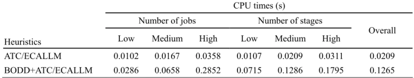
Finally, we take into consideration the efficiency of the bottleneck-based heuristics. All heuristics are coded in C++ language, and all experiments are performed on a PC with Pentium 4, 2.4 GHz CPU and 512 MB RAM. Table 8 displays the average computation time (in sec.) required for BODD+ATC/ECALLM to solve a problem. The results indicate that the average CPU time for BODD+ATC/ECALLM to solve a 100-job problem is less than 0.3 seconds, which is fast enough for it to be used in practice.

“Please Insert Table 7 about here” “Please Insert Table 8 about here” 3. Conclusions

This paper develops bottleneck-based heuristics to solve the FFL problem with unrelated parallel machines and with a bottleneck stage. The objective is to minimize the number of tardy jobs of the problem. Computational results have shown that the proposed bottleneck-based heuristics significantly outperform six well-known dispatching rules for the candidate problem. This is mainly contributed by the new approach for determining the arrival times of the jobs to the bottleneck stage and the decision rules for scheduling the jobs on the bottleneck stage. The results have also shown that the machine selection rule, ECALLM, should be used when the unrelated parallel machines are considered in the stages.

The experimental design has also found some interesting points. First, the effectiveness of BODD+ATC/ECALLM is robust to the problem size and to the variation of job processing time. Second, BODD+ATC/ECALLM is still effective even if the bottleneck phenomenon is not distinct. Third, the relative performance of BODD+ATC/ECALLM improves when the bottleneck stage is placed further back. Finally, BODD+ATC/ECALLM is very efficient and can be applied to real world problems.

As mentioned in the literature review, there are only a few research papers published on the FFL problem with unrelated parallel machines. These papers deal with the FFL problem considering different characteristics, such as sequence dependent setup times, and solve the problem using local search methods, such as simulated annealing and genetic algorithms. Therefore, this new bottleneck-based approach can be further applied to the FFL problem considering other characteristics, such as setup operations and reentrant processing; it can also consider other objectives such as total tardiness, total flow time, and makespan. Also, the new approach deserves to be applied to solve other scheduling problems with bottleneck stages. Furthermore, while conducting this research, we found that different methods for generating job’s processing time at each stage significantly affected the performance of the dispatching rules but not the performance of the proposed heuristics. For instance, the job’s processing time is generated with the assumption that the efficiency of the machines at a stage is consistent for all the jobs. None of the topics, considering the processing time information

on parallel processors, have been studied for the FFL problem with unrelated parallel machines. This is another interesting research topic.

Reference

Adler, L., Fraiman, N., Kobacker, E., Pinedo, M., Plotnicoff, J.C., and Wu, T.P., BPSS: A scheduling support system for the packaging industry. Operations Research. 1993, 41, 641–648.

Alisantoso, D., Khoo, L. P. and Jiang, P. Y., An immune algorithm approach to the scheduling of a flexible PCB flow shop. International Journal of Advanced

Manufacturing Technology, 2003, 22, 819–827.

Azizoglu, M., Cakmak, E. and Kondakci, S., A flexible flowshop problem with total flow time minimization. European Journal of Operational Research, 2001, 132, 528–538. Bertel, S. and Billaut, J. C., A genetic algorithm for an industrial multiprocessor flow shop

scheduling problem with recirculation. European Journal of Operational Research, 2004, 159, 651–662.

Brah, S. A., A comparative analysis of due date based job sequencing rules in a flow shop with multiple processors. Production Planning and Control, 1996, 7, 362–373.

Chen, Y. C. and Lee, C. E., Bottleneck-based group scheduling in a flow line cell.

International Journal of Industrial Engineering-Applications and Practice, 1998, 5,

288–300.

Choi, S. W., Kim, Y. D. and Lee, G. C., Minimizing total tardiness of orders with reentrant lots in a hybrid flowshop. International Journal of Production Research, 2005, 43, 2149–2167.

Conway, R., Comments on an exposition of multiple constraint scheduling. Production and

Operations Management, 1997, 6, 23–24.

Goldratt, E. and Fox, R., The Race. 1986 (North River Press: New York).

Goldratt, E. and Cox, J., The Goal: A Process of Ongoing Improvement. 1992 (North River Press: New York).

Hsieh, J.C., Chang, P.C., and Hsu, L.C., Scheduling of drilling operations in printed circuit board factory. Computers and Industrial Engineering, 2003, 44, 461–473.

Hunsucker, J. L., and Shah, J. R., Performance of priority rules in a due date flow shop.

Omega, 1992, 20, 73-89.

Jayamohan, M. S. and Rajendran, C., A comparative analysis of two different approaches to scheduling in flexibile flow shops. Production Planning and Control, 2002, 11, 216–230.

Jin, Z. H., Ohno, K., Ito, T. and Elmaghraby, S. E., Scheduling hybrid flowshops in printed circuit board assembly lines. Production and Operations Management, 2002, 11, 216–230.

Kadipasaoglu, S. N., Xiang, W. and Khumawala, B. M., A comparison of sequencing rules in static and dynamic hybrid flow systems. International Journal of Production Research, 1997, 35, 1359–1384.

Kim, D. W., Na, D. G. and Chen, F. F., Unrelated parallel machine scheduling with setup times and a total weighted tardiness objective. Robotics and Computer Integrated

Manufacturing, 2003, 19, 173–181.

Lee, G. C., Kim, Y. D., Kim, J. G. and Choi, S. H., A dispatching rule-based approach to production scheduling in a printed circuit board manufacturing system. Journal of the

Operational Research Society, 2003, 54, 1038–1049.

Lee, G. C., Kim, Y. D. and Choi, S. W., Bottleneck-focused scheduling for a hybrid flowshop.

Lenstra, J. K., Rinnooy Kan, A. H. G. and Brucker, P., Complexity of machine scheduling problems. Annals of Discrete Mathematics, 1977, 1, 343-362.

Linn, R. and Zhang, W., Hybrid flow shop scheduling: A survey. Computer & Industrial

Engineering, 1999, 37, 57–61.

Low, C. Y., Simulated annealing heuristic for flow shop scheduling problems with unrelated parallel machines. Computers and Operations Research, 2005, 32, 2013–2025.

Moore, J. M., Sequencing n jobs on one machine to minimize the number of tardy jobs.

Management Science, 1968, 15, 102–109.

Pinedo, M., Scheduling: Theory, Algorithms, and Systems. 2002 (Prentice-Hall, Upper Saddle River, New Jersey).

Ruiz, R. and Maroto, C., A genetic algorithm for hybrid flowshops with sequence dependent setup times and machine eligibility. European Journal of Operational Research, 2006, 169, 781–800.

Santos, D. L., Hunsucker, J. L. and Deal, D. E., Global lower bound for flow shops with multiple processors. European Journal of Operational Research, 1995, 80, 112–120. Sawik, T., An exact approach for batch scheduling in flexible flow lines with limited

intermediate buffers. Mathematical and Computer Modeling, 2002, 36, 461–471.

Yang, T., Kuo, Y. and Chang, I., Tabu-search simulation optimization approach for flow-shop scheduling with multiple processors – a case study. International Journal of Production

Research, 2004, 42, 4015–4030.

Yu, L., Shih, H. M., Pfund, M., Carlyle, W.M., and Fowler, J.W., Scheduling of unrelated parallel machines: an application to PWB manufacturing. IIE Transactions, 2002, 34, 921–931.

Table 1. Experimental Design for Generating Test Problems

Experimental Factor Factor Levels (low, medium, high)

Number of jobs 30, 50, 100

Number of stages 5, 10, 20

Variation of job processing time U[10,50], U[10,100], U[10,200]

Tightness of job due date U[0.1L, 0.9L], U[0.1L, 1.3L], U[0.1L, 1.7L],

Workload difference 1.1, 1.5, 2.0

Position of the bottleneck stage The first, second, and third quarter of the flow line

Table 2. Performance comparisons of the proposed heuristics and the dispatching rules (in terms of average RDI, average number of total tardy jobs (ATJ), and number of best solutions (NBS))

ATJ Average RDI (NBS)

Machine selection rules Machine selection rules

Heuristics

EAAM ECAM ECALLM EAAM ECAM ECALLM

SPT 39.21 25.63 20.52 0.8322 (0) 0.4063 (19) 0.2793 (66) EDD 45.35 25.52 17.58 0.9486 (0) 0.3631 (267) 0.1987 (711) MDD 40.46 19.07 15.35 0.8353 (0) 0.234 (182) 0.1483 (421) S/RPT+SPT 37.58 23.70 18.71 0.7869 (0) 0.3555 (21) 0.2346 (95) ATC 44.80 19.92 14.10 0.9388 (0) 0.2384 (352) 0.1162 (847) COVERT 41.47 19.78 15.56 0.8574 (0) 0.2506 (170) 0.1548 (385) BDD+ATC 34.21 11.47 10.11 0.6771 (1) 0.0360 (3548) 0.0095 (5560) BODD+ATC 34.40 11.68 10.07 0.6796 (3) 0.0379 (3805) 0.0077 (5981)

Table 3. Analysis of variance to test the significance of the machine selection rules (α=0.01).

Source of variation Degree of freedom Sum of squared error Mean squared error F**

Algorithms 7 2559331.23 365618.75 1213.07**

Machine selection rules 2 19821925.05 9910962.52 32883.17**

Error 174950 52729795.65 301.40

Total _{174959 75111051.92}

Table 4. Results of Duncan’s multiple range test for machine selection rules.

Machine selection rules ATJ Results (groups)

ECALLM 15.25 A

ECAM 19.59 B

EAAM 39.69 C

Table 5. Analysis of variance to test the significance of the algorithms when ECALLM is used (α=0.01).

Source of variation Degree of freedom Sum of squared error Mean squared error F**

Algorithms 7 727490.25 103927.18 850.14**

Error 58312 7128457.72 122.25

Total _{58319 7855947.98}

Table 6. Results of Duncan’s multiple range test for bottleneck-based heuristics.

Heuristics ATJ Results (groups)

BODD+ATC/ECALLM 10.07 A BDD+ATC/ECALLM 10.11 A ATC/ECALLM 14.10 B MDD/ECALLM 15.35 C COVERT/ECALLM 15.56 C EDD/ECALLM 17.58 D S/RPT+SPT/ECALLM 18.71 E SPT/ECALLM 20.52 F

Table 7. Effect of the experimental factors on the BODD+ATC/ECALLM (in terms of average RDI) Average RDI

Factors Low Medium High

Number of jobs 0.0075 0.0071 0.0086

Number of stages 0.0090 0.0072 0.0071

Processing time 0.0074 0.0072 0.0086

Due date tightness 0.0112 0.0062 0.0058

Workload difference 0.0099 0.0073 0.0060

Position of the bottleneck stage 0.0107 0.0073 0.0052

Table 8. Average computational time required for the heuristics CPU times (s)

Number of jobs Number of stages

Heuristics Low Medium High Low Medium High

Overall

ATC/ECALLM 0.0102 0.0167 0.0358 0.0107 0.0209 0.0311 0.0209