ROBUST STABILIZATION OF MULTIVARIABLE FEEDBACK-SYSTEMS WITH DESIRED PERFORMANCE REQUIREMENT

(1)

Robust stabilisation of multivariable feedback

systems with desired performance requirement

M.-H. TU C.-M. Lin

Indexing terms: Control systems, Internal stability, Robust stabilisation

Abstract: A design criterion is developed to achieve the following goals simultaneously: (i) input-output decoupling of multivariable feedback systems; (ii) complete and arbitrary closed-loop pole assignment; (iii) desired zero assignment for reference signal tracking; and (iv) robust stabilisation of multivariable feedback systems subjected to time-varying nonlinear uncertainties. Thus, the requirements of performance as well as stability robustness of a multivariable feedback system will be simultaneously met by employing this design criterion. Moreover, by minimising H"-norm of each channel of the closed-loop transfer matrix, we can obtain the robustness optimisation of the system, i.e., we can predict the maximum slope of the sector-bounded nonlinear uncertainties that can be tolerated in each channel of the system. A practical example, the lateral flight control of CCV (control configured vehicle), is given to illustrate the validity of the proposed design algorithm.

1 Introduction

In control systems the pole dominates the transient response as well as the system stability and so many studies [l,

21

have addressed pole assignment design. In addition, since the zero of a system plays an important role in the interaction between the system and its external environment, a great deal of research [3, 41 has gone into achieving reference signal tracking by assigning appropri- ate zeros. Thus, the pole-zero assignment of a control system is important for a system to achieve desired performance requirement. Another important control strat- egy is the robust stabilisation problem, i.e., the ability to maintain system stability under plant uncertainties. Cruz et al. [SI have discussed the robust stabilisation of linear feedback systems with time-varying nonlinear perturbations in terms of the roles of singular values. However their results are valid only when the plant and the controller are stable. Other work [ 6 , 71 uses the spectral norm to formulate an upper bound on the largest singular value of the closed-loop transfer matrix to guarantee

Paper 8696D (C8), first received 26th January 1991 and in revised form 2nd January 1992

M.-H. Tu is with the Institute of Electronics, National Chiao-Tung University, 1001 Ta-Hsueh Road, Hsin-Chu, 30050 Taiwan, Republic of China

C:M. Lin is with the Chung-Shan Institute of Science and Technology, PO Box 90008-6-5, Lung-Tan, Tao-Yuan 32500, Taiwan, Republic of China

IEE PROCEEDINGS-D, Vol. 139, No. 3, M A Y I992

robust stability of a multivariable control sytem under parameter variation. Dickman and Sivan [8] have shown that among the different, not necessarily diagonal, closed- loop transfer matrices which have the same diagonal ele- ments, the diagonal closed-loop transfer matrix has the greatest robustness for a multivariable system. Allowable perturbations are discussed in References 9 and 10 for maintaining stability of uncertain systems. These results are concerned only with stability robustness, they d o not deal with the robustness for maintaining a certain performance. Robustness results which do address the performance problem are found in References 11 and 12.

The primary purpose of this paper is to outline a design criterion for achieving the input-output decoupling (i.e. obtaining the diagonal closed-loop transfer matrices) of multivariable feedback systems and the robust stabilisation of systems subjected to time-varying nonlinear uncertainties with desired pole-zero assignment. By appropriately assigning the poles and zeros of the sensitivity matrix and simultaneously satisfying the robustness requirement, the proposed design algorithm ensures:

(i) input-output decoupling of multivariable feedback systems;

(ii) complete and arbitrary closed-loop pole assignment;

(iii) desired zero assignment for reference signal tracking;

(iv) robust stabilisation of multivariable feedback systems subjected to time-varying nonlinear uncertainties.

Moreover, by minimising H"-norm of each channel of the closed-loop transfer matrix, we can obtain the robustness optimisation of the system, i.e., we can predict the maximum slope of the sector-bounded nonlinear uncertainties that can be tolerated in each channel of the system.

The notations used in this paper are as follows: deg(*) denotes the degree of the polynomial

*.

diag(.) denotes a diagonal matrix.

11 11

denotes the Euclidean norm. The H"-norm of a transfer function G(s) is

/I G

I1

= sup

I

G ( j o )

1,

Vw E CO,

col

0

and B I B 0 stands for bounded-input bounded-output. 2 Problem formulation

Consider the multivariable feedback system subjected to time-varying nonlinear uncertainties shown in Fig. 1, where

p ,

P and C E C""" denote the practical plant, nominal plant and the controller, respectively. The time- varying nonlinear uncertainty A N [ u ( t ) , t] = diag

(2)

the control signal u ( t ) E R" and t E [0, w ] satisfying the following:

( a ) A N i [ O , t] = 0, i = 1,

. .

., n, for t E [0, so];

( b ) AN,[u(t), t], i = 1, . . . , n are measurable functions of (c) there exist finite constants pi > 0, i = 1,

.

, , , n with

I

A N i [ u ( t ) , tl

I

<

pz

I/

u(t)

11,

i = 1,

.

. . , nV /I u ( t )

11

< CO (1)

and the nonlinear uncertainties within the sectors having slopes p i , i = 1, .., n are denoted as A N i [ u ( t ) , t ] ,

f for all measerable u ( t ) ; and the property

I

Fig. 1 Multivariablefeedbark system with nonlinear unrertaintie~

i = 1, . . , n, and pi 11 u(t)

11,

i = 1, ..., n are the sector bounds of the nonlinear uncertainties.

Let the nominal plant of the system in Fig. 1 be factor- ised as

P ( s ) = A-'(s)B(s) = B , ( s ) A , ' ( s ) (2) where the pairs ( A ( s ) , B(s)) and (Bl(s), A , ( s ) ) are the left and right coprime polynomial matrix factorisations of the plant, respectively. The sensitivity matrix is defined as

S ( S ) =

(r

+

P ( ~ ) C ( S ) ) - I ₍₃₎

E(s) = S(s)R(s) (4)

then the tracking error signal E(s) can be obtained as

where R(s) is the reference signal. Let the reference signal R(s) = [rl(s), r2(s), ..., r,(s)]' and let the zeros of the polynomials mAs) be the poles of ri(s) in Re[s] 2 0 for i = 1, ..., n.

For the input-output decoupling, reference signal tracking and desired closed-loop pole assignment, the sensitivity matrix must be of the form

S(s) = diag [sl(s), . . . , s,(s)]

where yi(s), i = 1, , . . , n are Hurwitz polynomials with

desired closed-loop poles and wi(s), i = 1, . . . , n are unde- termined polynomials which should be determined to satisfy the internal stability constraints.

3

For application to any stable or unstable, minimum or nonminimum phase system, we first derive a pole-zero assignment control law which satisfies the internal stability of the multivariable feedback system in the nominal case, i.e. A N [ u ( t ) , t] = 0, for all t E [0, m].

Lemma f [ 1 3 ] : Suppose det ( A ( s ) ) and det ( B , ( s ) ) have no common zero in Re[s]

>

0. Then S(s) is internally stable if and only if S(s) is analytic in Re[s] 2 0 and for some appropriately dimensioned stable rational matrices X ( s ) and Y(s) such that

Pole-zero assignment control l a w design

S(s) = Y ( s ) A ( s ) I - S(S) = B1(s)X(s) S ( s ) A - 1(s) = Y ( s ) E ; '(s)(I - S(S)) = X ( S ) (8) (9) Equivalently, S(s) is internally stable if and only if S(s), S ( s ) A - l ( s ) and BF1(s)(I - S(s)) are all analytic in Re[s]

>

0.

Remark: If S(s) satisfies the requirements of internal stability, then we can directly obtain the controller as

(10) C(S) = P - ' ( s ) S - ' ( s ) ( z - S(s))

without worrying about any unstable hidden mode. Assume

A ' ( s ) = (1 1)

a,,(s) ' . ' a,A4

B ; '(s) =

b,i(s) ' ' ' bnAs)

From eqns. 5, 11 and 12, we obtain sl(s)all(s) ' . S l ( s ) w ) s,(s)a"l(s) . ' . s,(s)a,,(s) (1 - s,(s))b,,(s) ' ' ' (1 - s,(s))b,,(s) (1 - si(s))bni(s) ' . . (1 ~ sAs))b,,(s) (14) B , ' ( s ) ( l ~ S(S)) =

Define the polynomials 2 ,

I = '

ai(s) =

n

(s - pil)o", i = 1, . . . , n (15) where ii is the number of distinct poles p i l of the ith row of A - '(s) in Re[s] 2 0 and bi, is the greatest multiplicity of each pole p,l which appears in any element of the ith row of A '(s). Similarly, we define the polynomials

a,

1 = 1

pis)

=

fl

(s - qil)"Cf, i = I , .

. .

, n ₍₁₆₎ where 6; is the number of distinct poles qil of the ith column of B;'(s) in Re[s] 2 0 and q,l is the greatest multiplicity of each pole qil which appears in any element of the ith column of B,'(s). Then we obtain the following lemma:

Lemma 2: For the nominal system (i.e. A N [ u ( t ) , t] = 0) shown in Fig. 1, if &) and pi(s) are coprime for i = I,

. . .

, n, then S(s) = diag [sl(s),

. .

. , s.(s)] is internally stable if and only if the following conditions hold:

(i) si(s) is analytic in ReCs] 2 0 for i = 1,

.

. . , n ; (ii) the numerator polynomial of si(s) is divisible by

(iii) the numerator polynomial of 1 - si(s) is divisible ai(s) for i = 1, . . . , n ;

b y P i ( s ) f o r i = 1, ..., n.

Remark: If there exists any pair (ads), pi(s)) which is not coprime, then it is impossible for S(s) to achieve the internal stability.

From condition (ii) of Lemma 2, the numerator polynomial of s , ( ~ ) must contain ais), and from eqn. 5, the

(3)

I

numerator of s,(s) must also contain mi(s). Thus the numerator of si(s) must contain the least common multi- plier of q(s) and m,(s) for i = 1, . . , , n, i.e.,

where z,(s), i = 1,

.

. . , n are the least common multipliers of %is) and m i s ) while li(s), i = 1,

. . .

, n are undetermined polynomials. T o satisfy the requirement of causality of the closed-loop system, the sensitivity matrix must be proper, i.e.,

(18) deg (gi(s))

>

deg (li(s))

+

deg (zi(s)) i = 1,

.

. . , n From eqn. 17, we have

and from condition (iii) of Lemma 2, the numerator of 1 -

SAS)

must contain his). Thus we have

(20) his)

=

gis) - 1is)zis) = B X S ) f i ( S ) i = 1,

.

, , , n

wheref,(s), i = 1, .

. .

, n are undetermined polynomials Theorem I : The solution of li(s) in eqn. 20 exists if and only if mi(s) is coprime with

pi(s),

for i = 1, ,

. .

, n, respec-

tively.

Proof: (If): Since m i s ) is coprime with

bi(s),

and zi(s) is coprime with Bi(s), so that q(s) is coprime with P,(s); and since gis) is a Hurwitz polynomial and is coprime with

pis), so that the solution of li(s) in eqn. 20 exists, for

i = 1,

.

. _ , n. respectively.

(Only if): By contradiction, suppose mi(s) is not coprime with

pi(s),

so that zi(s) and

pi(s)

must have a common factor with zeros in Re[s] 0. And since gi(s) is a Hurwitz polynomial and is coprime with

pi(s),

hence the solution of li(s) in eqn. 20 does not exist, for i = 1,

. . .

,

n, respectively. This contradicts to the fact that the solu- tion of Ids) in eqn. 20 exists, so that mi(s) must be coprime with

pi(s).

Q E D .

Remark: If li(s) exists and the number of undetermined parameters of li(s) is equal to deg (pi(s)), then the solution of li(s) in eqn. 20 is unique for i = 1,

.

, n, respectively.

By solving eqn. 20, we obtain l,(s), i.e. S ( s ) is obtained Then the controller can be derived as

(21) Moreover, if li(s) exists and the number of undetermined parameters of l i s ) is greater than deg

(pis)),

then the solutions of [is) are not unique for i = 1,

. .

. , n, respectively. This leads to an over-parameterised solution and the free parameters of &) can be determined according

C(S) = P - ' ( s ) s - l ( s ) ( I - S(S))

to some specific performance criteria. In the following,

1,(s), i = 1, ..., n are determined to satisfy the stability

robustness requirement, and furthermore to minimise the H"-norm of each channel of the closed-loop transfer function to obtain the robustness optimisation of the system.

4

In the following, we consider the robust stabilisation of the feedback system subjected to sector-bounded nonlinear uncertainties.

Robust stabilisation of time-varying nonlinear uncertainties

Theorem 2 [SI: The feedback system in Fig. 1 is B I B 0 stable if

(i) S(s) is internally stable and (ii) pi 11 1 - si (1 I, < 1 for i = 1, . . . , n or

sup p , ( 1 - s i ( j o ) ( < 1 i = 1,.

. .

, n (22)

W t [ O . = I

Proof: For the proof of Theorem 2, refer to Reference 6. From the above analysis, the objective of the robust stabilisation control design of feedback systems subjected to sector-bounded nonlinear uncertainties is to adjust the controller C(s) such that the sensitivity function S ( s ) satisfies the internal stability of Lemma 2 with desired pole-zero assignment and the robust stability given in eqn. 22.

Thus, we obtain the following design algorithm for the robust stabilisation of multivariable feedback systems with desired performance requirement:

S t e p I : Perform the factorisation P(s) = A '(s)B(s) = B,(s)A; ' ( s ) and calculate A - ' ( s ) and B ; ' ( s ) , then determine d s ) and fli(s), for i = 1, . . . , n. And determine mi(s) and zi(s) as in eqn. 17.

Step 2: Choose diagonal sensitivity matrix S(s) = diag

[Sl(S), , , , ? s.(s)l.

Step 3: From eqn. 20, solve l,(s) and

h(s)

with free parameters, where gi(s), i = I , . . .

.

n are determined by the desired closed-loop poles for each channel.

Step 4 : By satisfying eqn. 22, determine the free parameters of li(s) in eqn. 19. And then S(s) is also determined.

Step 5 : Obtain the controller C(s) as in eqn. 21. Remark: Moreover, we can minimise 11 1 - si (1 ~, i = 1,

. .

. , n to obtain the robustness optimisation of the system with desired pole-zero assignment, i.e., we can predict the maximum slope

1 min

/I

1 - si

11

1.

Pi,,, =

of the sector-bounded nonlinear uncertainties that can be tolerated in each channel of the multivariable feedback system.

5 Example

A practical example, the lateral flight control of CCV (control configured vehicle) [14], is given to illustrate the validity of the proposed design algorithm.

The nominal lateral dynamics of T2-CCV can be decribed as follows: -0.259 0.039 0 ~ 1

0 0 1

-65.05 0 -3

-7.88 0 -0.05

0 0 0

(4)

the yaw angle (rad), 6, is the direct lift control angle (rad), 6, is the yaw rudder angle (rad), and 6, is the direct sideforce control angle (rad).

The transfer matrix form of the system can be obtained as

where

P(s)

-0.09(~ - 1.2001)(~

+

44.6357Xs

+

0.63442) P " ( S ) = ~ = S,(s) (s ~ 2.1987)(s - 0.10122)(s

+

2.0592)(s

+

3.9698) p(s) 0.121(s - 0.0080644)(s

+

131.941)(s

+

3.2726) P12(S) = - = 6,(~)

B(S)

6,(~) (S - 2.1987)(~ - 0.10122)(~

+

2.0592Xs

+

3.9698) 0.081(~ - 76.0459)(~ - 0.0345)(~

+

2.9332) (S ~ 2.1987X~ - 0.10122)(~

+

2.0592)(~

+

3.9698) PI 3(s) = - =

4(s)

1 5 1 ( ~ - 2.1035)(~

+

2.9206) P Z I ( S ) = ~ = P 2 2 N = - = 6 J s ) (s ~ 2.1987Xs - 0.10122)(s

+

2.0592)(s

+

3.9698) 4(s) 6 , ( ~ ) 46.2(~ - 5.5963)(~

+

5.451 1) (S ~ 2.1987)(~ - 0.10122Xs

+

2.0592)(~

+

3.9698) 4(s) S,(s) 7.106(s

+

0.8846

+

j6.9426)(s

+

0.8846 - j6.9426) (s ~ 2.1987Xs - 0.10122Hs

+

2.0592)(s + 3.9698) P 2 & ) = ~ = $(s) 6,(s) 3.654(s - 1.6984Xs

+

1.5426

+

j1.8985)(s

+

1.5426 - jl.8985) s(s - 2.1987)(s - 0.10122)(s

+

2.0592Xs

+

3.9698) P31(S) = ~ = +(s) - 15.94(s

+

3.469Ms - 0.0027

+

j0.994)(s - 0.0027 - j0.994) S(S ~ 2.1987)(~ - 0.10122)(~

+

2.0592)(~

+

3.9698) P 3 2 W = - = p&) = __ = 6,(S) $(s)

a"@)

6.206(s

+

3.1607Xs - 0.0309

+

j0.8309)(s - 0.0309 - j0.8309) s(s ~ 2.1987)(s - 0.10122)(s

+

2.0592)(s

+

3.9698)

Let us consider the system illustrated in Fig. 1 with the nominal plant P(s) described as above. We will synthesise a controller for:

( a ) decoupling the nominal system;

( b ) assigning five closed-loop system poles at - l/2 (c) tracking the unit step reference signal for each channel;

( d ) achieving the robust stabilisation of the sector-bounded nonlinear uncertainties

I

ANiCdt), t3 I

<

I1 u(r) I1

I ANzCu(tX

tl

I

<

3 I1

U@)

I/

I AN3Cu(t),

t l I

G $

I/

j(J(3)/2), - 8, - 12 and - 16 for channel 1, at -2

k

j2, - 12,

- 18 and -24 for channel 2, at - 1 j l , - 10, - I5 and -20 for channel 3 ;

I/

v

11

u ( t ) 11 <

Another design objective is to derive the maximum slopes p l m a x , pz,, and p3,x of the sector-bounded nonlinear uncertainties that can be tolerated in each channel of the feedback system under requirements (Q), (b) and (c).

(5)

0.3477(s + 3.1143)(s

+

0.8631)(s

+

0.2136) (s - 0.101 2Ks - 2.1987Ns + 3.9698Xs

+

2.0592)D(s) a i & ) = 0.0764(s - 4.344Ms

+

2.946Ks

+

0.0971) (S - 0.101 2Ns - 2.1987)(~

+

3.9698)(~

+

2.0592)D(~) a13(s) = -0.1188(~

+ 556.51)(~

+

4.107)(~

+

0.9785) (s - 0.1012)(s - 2.1987)(s

+

3.9698)(s

+

2.0592)D(s) (s - 2.6877Xs + 1.4582Xs

+

4.4471

+

j1.7138)(s

+

4.4471 - j1.7138) (s - 0.1012)(s - 2.1987)(s

+

3.9698)(s

+

2.0592)D(s) a,,is) = 4 s ) = az3(s) = 0.9168(~

+

5.8937)(~ - 1.4404)(~ - 0.2547) (S - 0.1012)(~ - 2.1987)(~

+

3.9698)(~

+

2.0592)D(s) -0.1639(s

+

51.846Xs + 4.0898)(s

+

2.4848)(s

+

0.02996) S(S - 0.1012)(~ - 2.1987)(~

+

3.9698)(~

+

2.0592)D(s) a 3 , ( s ) = 0.7017(~ - 3.0011)(~

+ 4.2938)(~

+

2.2135)(~

+

0.0842) S(S - 0.1012)(~ - 2.1987Hs

+

3.9698)(~

+

2.0592)D(s) a3&) = a33(s) = (S - 2.1827)(~

+

3.7006Xs

+

3.2746)(~

+

22.2119)(~ - 0.1020) s(s - 0.1012)(s - 2.1987)(s

+

3.9698)(s

+

2.0592)D(s) 400 (s

+

l)(s

+

2Xs

+

3)(s

+

5) b i i ( s ) = -2.0421(~

+ 3.8842)(~

- 19.167) D(s) b,,(s) = -2.8824 (s

+

3)(s

+

4Xs

+

5) b , 3(s) = -911 (s

+

1)(s

+

2)(s

+

3)(s

+

5) b z i ( S ) = -0.8545(~

+

3.8339)(~

+

130.91) D(4 M s ) = 12.871 (s

+

3Xs

+

4)(s

+

5) b23(s) - 2575.8 (s

+

1Xs

+

2)(s

+

3)(s

+

5) b31(s) = -0.9925(~

+

3.8398)(~

+

312.66) D(s) b,z(s) = - 22.429 (s

+

3)(s

+

4)(s

+

5) b33(s) = D(s) = (s

+

l)(s

+

2)(s

+

3)(s

+

4Ns

+

5)

Then we obtain ai@) and

Pis)

for i = 1, 2, 3 as follows:

r l ( s ) ( x ~ ( s ) = (S - 2.1987)(~ - 0.10122)

To satisfy the requirements (a), (b) and (c). the conditions (ii) and (iii) of Lemma 2, and the requirements of proper controller and causality of the closed-loop system, since pl(s) = 1, p 2 ( s ) = 1, and B3(s) = 1, we choose I,(s) = s2

+

39.2999s

+

p i , , 12(s) = s2

+

60.2999s

+

pZ1, and I&) = s2

+

49.2999s

+

p3,, with one undetermined parameter, respectively. Then the sensitivity matrix is chosen as

S i b ) 0

S ( S ) =

[

;

S Z ( 4

:

]

0 s3(4

(6)

S(S’

+

39.2999s

+

p 1 1 ) ( ~ - 0.10122)(~ - 2.1987) (s

+

8Xs

+

12Xs

+

16)(s2

+

s

+

1) Sl(S) = S Z ( 4 = S(S’

+

60.2999s

+

p 2 1 ) ( ~ - 0.10122)(~ - 2.1987) (s

+

12Ws

+

18Ns

+

24)(sz

+

4s

+

8) s(s2

+

49.2999s

+

p31)(s - 0.10122)(s - 2.1987) (s

+

l0Xs

+

15)(s

+

20)(s2

+

2s

+

2) =

For satisfying the stability robustness requirement, we have

$

sup 11 - sl(jw)l < 1, 41 < p l l < 244

3

sup ~ l - s 2 ( j w ) l < l , - 4 6 < p Z 1 < 9 0 3 w E IO. m l o E I O . m l $ sup 11 - s,(jw)l < 1, 164 < pS1 < 344 o E I O . m l

And the corresponding controller can be obtained as

c l l ( s ) c12(s) ‘13(’) C(S) = P - y s ) s - y s ) ( I - S ( S ) ) = ‘31(’) ‘32(‘) ‘ S S ( ’ ) where 4Oo(s - 0.1299) cll(s) = s(s - 0.10122)(s - 2.1987) (543.1641 - ~ 1 1

+

)(1979.2537 ~ ~

+

2.2999p11)s2

+

(1952 - 0.2226~11)~

+

1536 s2

+ 39.2999s

+

p l l -2.0421(s

+

1.5353

+

j2.2983Xs

+

1.5353 - j2.2983) S(S - 0.10122)(~ - 2.1987) ClZ(S) = (1298.462 - ~ 2 1

+

)(9346.58 ~ ~

+

2.2999p21)s2

+

(28224 - 0.2226p21)~

+

41472 s2

+

60.2999s

+

p21 -2.8824s - 139.7452) (S - 0.10122X~ - 2.1987) c13(s) = (855.1633 - ~ 3 1 ) ~ ’

+

(4379.0282

+

2 . 2 9 9 9 ~ 3 1 ) ~ ~

+

(7300 - 0.2226p31)~

+

6300 sz

+

49.2999s

+

pSl -911.14(~

+

0.2087) S(S - 0.10122Xs - 2.1987) c 2 1 ( 4 = (543.1641 - pll)s3

+

(1979.2537

+

2 . 2 9 9 9 ~ ~ ~ ) ~ ~

+

(1952 - 0.2226p11)s

+

1536 sz

+

39.2999s

+

p l l -0.8545(~

+

7.6692)(~ - 5.4223) S(S - 0.10122Xs - 2.1987) c 2 2 ( s ) = (1298.462 - p21)s3

+

(9346.58

+

2.2999p21)s2

+

(28224 - 0.2226p2,)~

+

41472 s2

+

60.2999s

+

p21 12.871(~ - 70.1873) ( S - 0.10122)(~ - 2.1987) c23(s) = (855.1633 - p31)sS

+

(4379.0282

+

2.2999p31)s2

+

(7300 - O.2226pS1)s

+

6300 s2

+

49.2999s

+

p31 -2575.8(~

+

0.3527) S(S - 0.10122)(~ - 2.1987) c31(s) = (543.1641 - pll)s3

+

(1979.2537

+

2.2999pll)s2

+

(1952 - 0 . 2 2 2 6 ~ ~ ~ ) ~

+

1536 sz

+

39.2999s

+

p l l 264

(7)

-0.9925(~

+

12.3354Xs - 8.2054) s(s - 0.10122Xs - 2.1987) c3Z(s) = (1298.462 - pZ1)s3

+

(9346.58

+

2.2999pZ1)s2

+

(28224 - 0.2226pZl)s

+

41472 sz

+

60.2999s

+

pz1 -22.429(~

+

115.2201) (S - 0.10122Xs - 2.1987) c 3 3 ( 4 = (855.1633 - p 3 J s 3

+

(4379.0282

+

2 . 2 9 9 9 ~ ~ ~ ) ~ ~

+

(7300 - 0.2226p3,)s

+

6300 s2

+

49.2999s

+

p31 Moreover, min sup 11 - sl(jw)l = 1.3719, p l l = 153 (33)

min sup 11 - sz(jo)l = 1.4252, pzl = 385 (34)

min sup 11 - s 3 ( j o ) l = 1.3625, p31 = 254 (35)

CIS) O E IO. m1

CIS1 w t IO, ml

C(sl O E IO. ml

And then the maximum slopes of the sector-bounded nonlinear uncertainties that can be tolerated in this system are pl,, = (lp.3719) = 0.7289, p2,, =

(1/1.4252) = 0.7017, and p3,., = (1/1.3625) = 0.7339. That is if no nonlinear uncertainty exists-AN[u(t), t ] = 0, for all t E CO. col-and we choose the controller as in eqn. 32 with arbitrary real p l l , pzl and p31, then the feedback system in Fig. 1 achieves internal stability with desired pole-zero assignment. And if there exist nonlinear uncer-

5

tainties within the sector bound with slopes p1 = (2/3),

E

p 2 = (3/5) and p 3 = (5/7), we choose the controller as in h eqn. 32, by satisfying inequalities eqns. 29, 30 and 31,

5

then the feedback system in Fig. 1 also achieves robust .E- stability. Moreover, when we choose the controller as in eqn. 32 with p l , = 153, pzl = 385 and pLSl = 254, then - the feedback system in Fig. 1 can tolerate the nonlinear uncertainties within the maximum sector bound with -

slopes pl,, = 0.7289, pz,, = 0.7017 and p3,, = 0.7339. The Nyquist diagrams of the loop gain for channel 1 with p l l = 41, 153 and 244 are shown in Fig. 2. Since the loop gain with p I I = 41 and 244, respectively, has two Fig. 2, the Nyquist diagram of the loop gain with p I 1 = clockwise direction, then the circle disk which intersects

-6 -4 -2 0

-4 -8

real part poles (2,1987 and 0.1012) in the right-half plane and from

41 and 244, completely encircles twice in a counter-

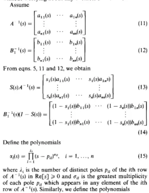
Fig. 3

~~~.

diagram Of the loo?’ gainfor channel

’

p 2 , = -46 (dashed line)

p 2 , = 385 (solid line) p 2 , = 903 (dashdot Line)

~

real p a r i

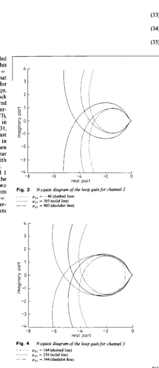
Nyquist diagram of the loop gainfor channel 3 Fig. 4

p,, = 164 (dashed line)

~ p 3 , = 254 (solid Line)

pa, = 344 (dashdot line)

~ . - ~

(8)

and [ - l/(l

+

(2/3))] = -0.6 corresponds to the slope

pl

= (2/3) of the sector-bounded uncertainty AN,[u(t), t3 in the feedback system. Moreover, the loop gain for p I 1 = 153 also has two poles (2.1987 and 0.1012) in the right-half plane, and from Fig. 2, the Nyquist diagram of the loop gain for p l , = 153 completely encircles twice in counterclockwise direction, the circle disk which intersects the real axis at boundary values [ - l/(l - 0.7289)] = -3.6887 and [ - l/(l

+

0.7289)] = -0.5784 corresponding to the maximum slope pi,, = 0.7289 of the sector-bounded uncertainty A N I [ u ( t ) , t]

that can be tolerated in the feedback system. These satisfy the circle criterion and Nyquist criterion, thus the robust stability is ensured. Similarly, the Nyquist diagrams of the loop gain for channels 2 and 3 with pz1 = -46, 385 and 903 and p31 = 164,254 and 344 shown in Figs. 3 and 4 also satisfy the circle criterion and Nyquist criterion, thus the robust stability is ensured.

6 Numerical algorithm for controller design

The computer-aided-design package MATLAB has been used for the numerical computations in this paper. The numerical algorithm for controller design in the preced- ing Sections includes:

( a ) conversion of a system from a state-space model to transfer function matrix form;

(b) left and right coprime factorisations of a transfer function matrix;

(c) inversion of a transfer function matrix; ( d ) H“-norm calculation of a transfer function. For Item (a), an M-file [l5] is written by using the state-space to transfer function conversion function of the MATLAB Control System Toolbox.

For Item (b), the algorithm given in Reference 16 (Section 4.1) is adopted to design an M-file to obtain the left and right coprime factorisations of a transfer function matrix.

For Item (c), an M-file is written to construct the adjoint matrix and the determinant of a transfer function matrix by using the convolution function of the MATLAB toolbox. For a rational matrix which is proper and not strictly proper, a more efficient algorithm given in Reference 16 (Section 7.1) is used to design an M-file to obtain the inverse of a transfer function matrix.

For Item

(4,

the algorithm given in Reference 17 is adopted to design an M-file to calculate the H“-norm of a transfer function by using the transfer function to state- space conversion function of the MATLAB control system toolbox and the eigenvalue function of the MATLAB toolbox.

A design criterion has been developed to simultaneously consider the performance and the stability robustness o f a multivariable feedback system. Moreover, by minimising H“-norm of each channel of the closed-loop transfer matrix, we can predict the maximum slope of the sector-bounded nonlinear uncertainties that can be tolerated in each channel of the feedback system. Since the requirements of internal stability are satisfied, this design algorithm performs appropriately, even if the plant is unstable and/or nonminimum phase.

8 References

1 CHEN, C.-T.: ‘Linear system theory and design’ (Holt, Rinehart & Winston, 1984)

2 ASTROM, K.J., and WITTENMARK, B.: ’Computer controlled systems’ (Prentice-Hall, 1990)

3 WOLOVICH, W.A.: ‘Multipurpose controllers for multivariable systems’, IEEE Trans., 1981, AC-26, pp. 162-170

4 SAEKS, R., and MURRAY, J.: ’Feedback system design: the track- ing and disturbance rejection problem’, IEEE Trans., 1981, AC-26, p. 203-217

5 CRUZ, J.B., FREUDENBERG, J.S., and LOOZE, D.P.: ‘A relationship between sensitivity and stability of multivariable feed- back systems’, IEEE Trans., 1981, AC-26, pp. 66-74

6 DOYLE, J.C., and STEIN, G.: ‘Multivariable feedback design: con- cepts for a classicalJmodern synthesis’, IEEE Trans., 1981, AC-26, pp. 4-16

7 CHEN, M.J., and DESOER, C.A.: ‘The problem of guaranteeing robust disturbance rejection in linear multivariable feedback systems’, Int. J. Control, 1983.. 37, pp. 305-313

8 DICKMAN, A., and SIVAN, R.: ‘On the robustness of multi- variable feedback systems’, IEEE Trans., 1985, AC-30, pp. 401-404 9 YEDAVALLI, R.K., and LIANG, Z.: ‘Reduced conservatism in sta-

bility robustness bounds by state transformation’, IEEE Trans., 1986, AC-31, pp. 863-866

10 ZHOU, K., and KHARGONEKAR, P.P.: ‘Stability robustness bounds for linear state space models with structured uncertainty’.

IEEE Trans., 1987, AC-32, pp. 621-623

11 HYLAND, D.C., and BERNSTEIN, D.S.: ‘The majorant Lyapu- nov equation: a non-negative matrix equation for robust stability and performance of large scale systems’, IEEE Trans., 1987, AC-32, pp. 1005-1013

12 COLLINS, E.G. Jr., and HYLAND, D.C.: ‘Improved robust performance bounds in covariance majorant analysis’. Proc. 27th IEEE C o d . Decision Contr., 1988, pp. 2188-2193

13 SAFONOV, M.G., and CHEN, B.S.: ’Multivariable stability-margin optimisation with decoupling and output regulation’, IEE Proc. D ,

Control Theor)’ & .4pp1., 1982,129, pp. 276-282

14 KANAI, K., and UCHIKADO, S.: ‘An adaptive flight control system design for CCV with an unknown interactor matrix’, J. Jn.,

Aeronaut. & Astronaut. Assoc., 1986,34, (387), pp. 211-221 15 ‘PC-MATLAB user’s guide, version 3.5’ (The Mathworks, Inc.,

South Natick, MA, USA, 1990)

16 FRANCIS, B.A.: ‘A course in H“ control theory’ (Springer-Verlag, 1987)

17 DOYLE, J.C., GLOVER, K., KHARGONEKAR, P.P., and FRANCIS, B.A.: ‘State-space solutions to standard H’ and H“ control problems’, IEEE Trans., 1989, AC-34, pp. 831-847