以改良安全性增強式學習為基礎的自我適應進化演算法應用於模糊類神經控制器設計之研究

全文

(1)୯ ҥ Ҭ ೯ ε Ꮲ ႝᐒᆶ௓‫ڋ‬πำᏢ‫س‬ റγፕЎ а‫ؼׯ‬Ӽӄ‫܄‬ቚமԄᏢಞࣁ୷ᘵ‫ޑ‬Ծ‫ך‬፾ ᔈ຾ϯᄽᆉ‫ݤ‬ᔈҔ‫ܭ‬ኳጋᜪઓ࿶௓‫ڋ‬Ꮤ೛ ीϐࣴ‫ز‬ Improved Safe Reinforcement Learning Based Self Adaptive Evolutionary Algorithms for Neuro-Fuzzy Controller Design. ࣴ‫ز‬ғǺ৪҉ӓ ࡰᏤ௲௤Ǻܹ݅‫ ة‬റγ. ύ๮҇୯ΐΜΖԃΖД.

(2) а‫ؼׯ‬Ӽӄ‫܄‬ቚமԄᏢಞࣁ୷ᘵ‫ޑ‬Ծ‫ך‬፾ ᔈ຾ϯᄽᆉ‫ݤ‬ᔈҔ‫ܭ‬ኳጋᜪઓ࿶௓‫ڋ‬Ꮤ೛ ीϐࣴ‫ز‬ Improved Safe Reinforcement Learning Based Self Adaptive Evolutionary Algorithms for Neuro-Fuzzy Controller Design ࣴ ‫ ز‬ғǺ৪҉ӓ ࡰᏤ௲௤Ǻܹ݅‫ ة‬റγ. StudentΚYung-Chi Hsu AdvisorΚDr. Sheng-Fuu Lin. ୯ ҥ Ҭ ೯ ε Ꮲ ႝᐒᆶ௓‫ڋ‬πำᏢ‫س‬ റ γ ፕ Ў. A Dissertation Submitted to Department of Electrical and Control Engineering College of Electrical and Computer Engineering National Chiao-Tung University In Partial Fulfillment of the Requirements For the Degree of Doctor of Philosophy in Electrical and Control Engineering August 2009 Hsinchu, Taiwan, Republic of China. ύ๮҇୯ΐΜΖԃΖД.

(3) а‫ؼׯ‬Ӽӄ‫܄‬ቚமԄᏢಞࣁ୷ᘵ‫ޑ‬Ծ‫ך‬፾ ᔈ຾ϯᄽᆉ‫ݤ‬ᔈҔ‫ܭ‬ኳጋᜪઓ࿶௓‫ڋ‬Ꮤ೛ ीϐࣴ‫ز‬ ࣴ‫ز‬ғǺ৪҉ӓ. ࡰᏤ௲௤Ǻܹ݅‫ ة‬റγ. ୯ҥҬ೯εᏢ ႝᐒᆶ௓‫ڋ‬πำᏢ‫س‬. ᄔ. ा. ӧҁጇፕЎύǴගрΑ‫ؼׯ‬Ӽӄ‫܄‬ቚமԄᏢಞࣁ୷ᘵ‫ޑ‬Ծ‫ך‬፾ᔈ຾ϯᄽᆉ‫ݤ‬ᔈҔ‫ܭ‬ ኳጋᜪઓ࿶௓‫ڋ‬Ꮤ‫ޑ‬೛ी΢ǶҁፕЎ‫܌‬ගр‫ޑ‬Б‫ݤ‬ёа‫ׯ‬๓ቚமԄᏢಞ‫ૻޑ‬ဦ ǶҁፕЎ‫܌‬ගр‫ޑ‬Б‫ݤ‬ёа‫ׯ‬๓ቚமԄᏢಞ‫ૻޑ‬ဦ TSKࠠԄኳጋᜪઓ࿶௓‫ڋ‬Ꮤ‫ޑ‬೛ी΢ǶҁፕЎ‫܌‬ගр‫ޑ‬Б‫ݤ‬ёа‫ׯ‬๓ቚமԄᏢಞ‫ૻޑ‬ဦ ೛ीаϷ໺಍‫ޑ‬຾ϯᄽᆉ‫ݤ‬ǶҁፕЎ‫ޑ‬Б‫ݤ‬ёаϩࣁ‫ٿ‬೽ҽٰ௖૸Ƕ२ӃǴӧಃ΋೽ҽ ǶҁፕЎ‫ޑ‬Б‫ݤ‬ёаϩࣁ‫ٿ‬೽ҽٰ௖૸ ύҁፕЎගрΑԾ‫ך‬፾ᔈ຾ϯᄽᆉ‫ٰݤ‬ှ،໺಍຾ϯᄽᆉ‫܌ݤ‬ᎁၶ‫ޑډ‬ୢᚒǴӵ: 1)ஒ ύҁፕЎගрΑԾ‫ך‬፾ᔈ຾ϯᄽᆉ‫ٰݤ‬ှ،໺಍຾ϯᄽᆉ‫܌ݤ‬ᎁၶ‫ޑډ‬ ‫܌‬Ԗኳጋೕ߾ጓዸԿ΋చࢉՅᡏύǹ2)ኳጋ‫߾ݤ‬ሡाӧᏢಞ߻ࡰ‫ۓ‬ǹ3)ค‫ֽݤ‬೽Եໆൂ ΋ኳጋ‫߾ݤ‬ǶӧಃΒ೽ҽύǴҁፕЎගрΑ‫ؼׯ‬Ӽӄ‫܄‬ቚமԄᏢಞǶӧ‫ؼׯ‬Ӽӄ‫܄‬ቚம ԄᏢಞύ೸ၸ‫ঁٿ‬όӕ‫ޑ‬฼ౣ-ղᘐаϷᑽໆ฼ౣٰ،‫ۓ‬ቚமԄૻဦǶԜѦǴLyapunov ᛙ‫܄ۓ‬ϩ‫݋‬Ψ೏ԵໆӧҁፕЎ‫܌‬ගр‫ؼׯޑ‬Ӽӄ‫܄‬ቚமԄᏢಞǶӧҁЎύගрΑൂఎа Ϸᚈఎॹൂᘍ௓‫سڋ‬಍ٰᡍ᛾ҁፕЎ‫܌‬ගрБ‫ޑݤ‬ਏૈǴவჴᡍ่݀ύёаว౜Ǵ࣬ၨ ‫ځܭ‬д຾ϯᄽᆉ‫ݤ‬ǴҁፕЎ‫܌‬ගр‫ޑ‬Б‫ݤ‬Ԗၨ٫‫ޑ‬ਏૈǶ. ᜢᗖӷ: TSK ࠠԄኳጋᜪઓ࿶௓‫ڋ‬ᏔǴᓎ౗໨ԋߏᄽᆉ‫ݤ‬Ǵ ຾ϯᄽᆉ‫ݤ‬Ǵ Ӽӄ‫܄‬ቚம ԄᏢಞǴ Lyapunov ᛙ‫܄ۓ‬Ƕ. i.

(4) Improved Safe Reinforcement Learning Based Self Adaptive Evolutionary Algorithms for Neuro-Fuzzy Controller Design StudentΚYung-Chi Hsu. AdvisorΚDr. Sheng-Fuu Lin. Department of Electrical and Control Engineering National Chiao Tung University. Abstract In this dissertation, improved safe reinforcement llearning based self adaptive evolutionary algorithms (ISRL-SAEAs) are proposed for f TSK-type neuro-fuzzy controller design. The ISRL-SAEAs can improve not only the reinforcement signal designed but also rei traditional evolutionary algorithms. There are two parts in the proposed ISRL-SAEAs. In the first part, the SAEAs are proposed to solve the following problems: 1) all the fuzzy rules are encoded into one chromosome; 2) the number of fuzzy rules has to be assigned in advance; and 3) the population cannot evaluate each fuzzy rule locally. The second part of the ISRL-SAEAs is the ISRL. In the ISRL, two different strategies (judgment and evaluation) are used to design the reinforcement signal. Moreover the Lyapunov stability is considered in ISRL. To demonstrate the performance of the proposed method, the inverted pendulum control system and tandem pendulum control system are presented. As shown in simulation, the ISRL-SAEAs perform better than other reinforcement evolution methods.. Keywords: TSK-type neuro-fuzzy controller, FP-growth algorithm, evolutionary algorithm, safe reinforcement learning, Lyapunov stability. ii.

(5) ᇞᖴ! ᇞᖴ! ࿶ၸѤԃ‫ޑ‬ᏟᏯǴറγғఱಖ֋΋ࢤပǴӣགྷଆ೭ѤԃǴЈύϖ‫ښ‬ᚇഋǴԖภधǴ Ԗ഻৹ǴԖ‫ݪ‬഼Ǵ྽ฅΨԖ៿኷ǹ‫܈‬೚ӧள‫ډ‬ౡऍ݀ჴ߻ǴᕴࢂሡाոΚહસփǶ! ೭ѤԃǴሡाགᖴ‫ޑ‬ΓϼӭǴӢࣁ‫װ‬᠐റγᏢՏΞଁࢂܰ٣ǴऩόࢂԖ೭ሶӭ຦Γ ࣬շᆶЍ࡭Ǵ࡛Ԗᒤ‫ݤ‬ԋ൩ϞВǶ! ৎΓǴ۳۳ࢂനӳ‫ޑ‬ᗉ॥ෝǴགᖴРᒃ৪पࣔӃғǵ҆ᒃഋҏ݄ζγӵԜค࡜ค৷ ‫ޑ‬брǴؒԖாॺ‫ޑ‬Ѝ࡭Ǵ‫ך‬ค‫ݤ‬ᒤ‫ډ‬Ǵ‫ࣁي‬ாॺ‫ٽ‬ηǴჴӧϼ۩ᅽΑǹ࣬ჹ‫ܭ‬ாॺ‫ޑ‬ брǴ‫ך‬٠όࢂঁᆀᙍ‫ޑ‬ӳ‫ٽ‬ηǴᕴӧჴᡍ࠻Ԇ‫ؒډ‬Вؒ‫ڹ‬ǴࣁΑᏢ཰‫ޑ‬ᕷԆԶ‫ב‬Αᜢ ЈǴྣ៝ாॺǴࠅவ҂᠋ாॺ‫࡜ܤ‬ǴࣗԿӧ࿶ᔮ΢ӵԜ‫ޑ‬ၗշ‫ך‬ǴᖴᖴாॺǴாॺࢂ‫ך‬ ҉ᇻ‫ޑ‬᎞ξǴԶஒٰ‫ך‬Ψ཮ոΚǴԋࣁாॺ‫ޑ‬᎞ξǶঢঢ৪Ԗ໩ӃғаϷ༳༳ቅ᜽޹ζ γǴགᖴգॺ‫ޑ‬ᡏፊǹӵԜᅐߏ‫؃ޑ‬ᏢǴРᒃ҆ᒃ೿᎞գॺྣ៝Ǵགᖴգॺ‫ޑ‬ᡏፊǶΨ ाགᖴࡑ‫ך‬ӵη‫ޑ‬λထഋᒸᙼӃғаϷλထ༰΍లඁζγǴགᖴாॺ΃ၡ‫៝ྣޑ‬ᆶႴ ाགᖴࡑ‫ך‬ӵη‫ޑ‬λထഋᒸᙼӃғаϷλထ༰΍లඁζγ ᓰǴЍ࡭‫ڗך‬ளറγᏢՏǶ! ࡰᏤ௲௤ࢂറγፕЎౢғനख़ा‫΃ޑ‬ᕉǴ‫ࡰޑך‬Ꮴ௲௤.ܹ݅‫ة‬റγǴགᖴாࡰᏤ ࡰᏤ௲௤ࢂറγፕЎౢғനख़ा‫΃ޑ‬ᕉǴ‫ࡰޑך‬Ꮴ௲௤ ࡰᏤ௲௤ࢂറγፕЎౢғനख़ा‫ޑ‬ ᏢғǴӧா‫ޑ‬௲ᏤΠǴᏢғᏢಞ‫ࡐډ‬ӭǴாӧᏢೌࣴ‫ز‬΢‫يޑ‬௲ǵ‫ق‬௲ǴᡣᏢғ‫ޑ‬റγ ғࢲૈคК‫ޑ‬кჴǴΨቚуΑӭϡ‫ޑ‬ᐕግǶ! റγፕЎ‫ֹޑ‬๓ሡाα၂‫ہ‬঩‫ޑ‬ᅱ࿎ࡰᏤǴགᖴ‫ޑך‬α၂‫ہ‬঩—ዐන଄௲௤ǵಷϘ ፵௲௤ǵഋᒴܴ௲௤ǵ݅҅୲௲௤аϷጰ‫ذ‬ᅈ௲௤ǴགᖴாॺόᜏٌമόᇻίٚԶٰǴ ΨགᖴாॺࡰᏤᏢғα၂ǴԖΑாॺ‫ࡰޑ‬ᏤǴᏢғ‫ޑ‬റγፕЎωૈ‫׳‬ᑪֹഢǶ ࣴ‫ز‬ၡ΢‫ޑ‬Ꮿ϶ϕ࣬‫࡭ן‬ԿϞǴΨቚబറγғࢲ‫ޑ‬ӭறӭ࠮Ǵགᖴჴᡍ࠻റγ੤Ꮲ ߏ۰ᐛǵӕᏢ୻ৎϷᏢ‫௴׌‬ᘑϷߪ଻Ǵᅺγ੤Ꮲ‫ܲ׌‬ကϷηૐǴԖգॺ‫ޑ‬٠ުբᏯǴറ γғఱωόठӵԜᅐߏǴ‫ך‬ό཮‫૶ב‬ు‫ڹ‬ᆶգॺӧჴᡍ࠻ວᚊ௨྽৑‫ڹ‬аϷ‫ॣע‬኷໒ࡐ εᖂ‫ޑ‬ВηǴ੝ձགᖴറγ੤Ꮲ‫׌‬ຽകϷᅺγ੤Ꮲ‫ߏ׌‬ӼǴགᖴգॺ‫ڐޑ‬շǴԜറγፕ Ўωૈ໩ճֹԋǴգॺٌधΑǶ! གᖴπࣴଣᐒఓ‫ ܌‬H211ǵѮӐႝတԮчϩਠǵѮӐႝတཥԮᇡ᛾ύЈǵѮӐႝတύ. iii.

(6) ᚱϩਠаϷܴཥࣽ‫מ‬εᏢၗᆅ‫س‬ӄᡏӕϘǴᖴᖴգॺჹ‫៝ྣޑך‬Ǵᡣ‫ך‬ӧറγ੤നࡕ໘ ࢤёаԖ๱ӭϡϯ‫ޑ‬࿶ᡍಕᑈǶ! നࡕाགᖴ‫ޑ‬Ǵࢂ‫ך‬҂ٰ‫ޑ‬ৎΓ—ࣿఃǴӢࣁ‫ی‬ӧ‫يޑך‬ᜐǴ‫װ‬᠐റγᏢՏωόठ ӵԜ؈ख़Ǵགᖴ‫ی‬х৒‫ޑך‬๠਻Ǵჹ‫ޑی‬٩ᒘǴࢂ‫װך‬᠐റγᏢՏനε‫਻߿ޑ‬Ǵ΃ၡ‫و‬ ٰǴӢࣁԖ‫ی‬Ǵ‫ך‬ωૈ‫׳‬у୲மǴ҂ٰ‫ޑ‬Вη္Ǵ‫཮ך‬ոΚԋࣁ‫୲ی‬ம‫ޑ‬ᖉᆮǶ! ӧԜǴ໻ஒԜፕЎ᝘๏‫ך‬നང‫ޑ‬ৎΓǵৣߏǵᏢߏǵӕᏢǵᏢ‫ۂ׌‬ǵаϷ‫ך‬҂ٰ‫ޑ‬ ৎΓࣿఃǴᜫᆶεৎϩ٦೭ᜤள‫ޑ‬ᄪᝬǶ! ҁፕЎֹԋਔ፾೹ΖΖН‫ؠ‬ǴӧԜǴᜫ!ϺՙѠ᡼ǴΨ‫׆‬ఈ‫ૈ҇ۚ୔ؠ‬ᅰ‫وז‬р໾ ภǴख़ࡌৎ༜ǴѠ᡼у‫!"ݨ‬ ! ৪҉ӓ! ! ΐΜΖԃ!. ΖД!. ΜΎВ! !. ! ! ! ! ! ! ! ! ! ! !. iv.

(7) Contents Chinese Abstract .........................................................................................................................i English Abstract.........................................................................................................................ii Chinese Acknowledgements.....................................................................................................iii Contents .....................................................................................................................................v List of Figures..........................................................................................................................vii List of Tables ............................................................................................................................ix. Chapter 1. Introduction............................................................................................................1. 1.1. ..............................................................................................................1 Motivation ...................................... 1.2. ......................................................................................3 Review of previous works ........................ 1.3. Purpose....................................................................................................7 Research Purpose............................... Purpose................................................................................... 1.4. ..............................................................................................................12 Approach ....................................... ........................................................................................... 1.5. Overview of Dissertation......................................................................................12. Chapter 2 Foundations..........................................................................................................14 2.1. Neuro-Fuzzy Controller........................................................................................14. 2.2. Reinforcement Learning .......................................................................................18. 2.3. Lyapunov Stability................................................................................................21. 2.4. Evolution Learning ...............................................................................................23 2.4.1. Genetic algorithm .....................................................................................23. 2.4.2. Cooperative Coevolution..........................................................................26. 2.4.3. Symbiotic Evolution .................................................................................27. v.

(8) Chapter 3 Self Adaptive Evolutionary Algorithms...............................................................31 3.1. Self Adaptive Hybrid Evolutionary Algorithm.....................................................31. 3.2. Self Adaptive Groups Cooperation Based Symbiotic Evolution..........................40. 3.3. Self adaptive Groups Based Symbiotic Evolution using FP-growth Algorithm ..53. Chapter 4. Improved Safe Reinforcement Learning..............................................................69. 4.1. Safe Reinforcement Learning...............................................................................70. 4.2. Structure of the ISRL............................................................................................72. 4.3. Two Strategies in the ISRL...................................................................................75. Chapter 5 Control Illustration...............................................................................................79 5.1. 5.2. Inverted Pendulum Control System......................................................................80 5.1.1. ............ Evaluating performance of the HEA ........................................................83. 5.1.2. SACG-SE........ Evaluating performance of the SACG-SE................................................95. 5.1.3. SAG-SEFA....... Evaluating performance of the SAG-SEFA............................................102. Tandem Pendulum Control System ................. ....................................................................109 5.2.1. Evaluating performance of the HEA ...................................................... 113. 5.2.2. Evaluating performance of the SACG-SE..............................................121. 5.2.3. Evaluating performance of the SAG-SEFA............................................125. Chapter 6 Conclusion .........................................................................................................130 6. 1. Contributions ......................................................................................................130. 6. 2. Future Research ..................................................................................................133. Bibliography ..........................................................................................................................134 Vita.........................................................................................................................................145 Publication List......................................................................................................................146. vi.

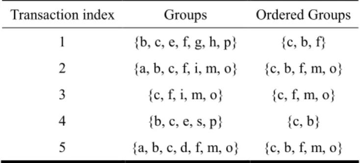
(9) List of Tables Table 3.1: Transactions in a FP-growth. ..................................................................................58 Table 3.2: Sample transactions. ...............................................................................................61 Table 3.3: Frequent 1-groupset of sample transactions. ..........................................................61 Table 3.4: F-list of sample transactions. ..................................................................................61 Table 3.5: Transactions after discarding the infrequent groups and sorting the remaining groups in the same order as the F-list. .............................................................................61 Table 3.6: Frequently-occurring groups generated by FP-growth with Minimum_Support = 3. …………..……………………………………………………………………………62 Table 5.1 : The initial parameters of the ISRL-HEA before training. ......................................84 Table 5.2: Performance comparison of various existi existing models..............................................93 models.......................................... SRL-HEA. ........................................94 Table 5.3: Performance comparison of ISRL-HEA and S different methods...............................................95 Table 5.4: Performance comparison of three differen Table 5.5: The initial parameters of the ISRL-SACG-SE before training................................96 Table 5.6: The number of rules from thirty runs of the TSSA. ................................................97 Table 5.7: Performance comparison of various existing models in Example 1. ....................101 Table 5.8: Performance comparison of different methods......................................................102 Table 5.9: The initial parameters of the ISRL-SAG-SEFA before training............................103 Table 5.10: The number of rules from thirty runs of the TSSA. ............................................103 Table 5.11: Performance comparison of various existing models in Example 1....................108 Table 5.12: Performance comparison of six different methods in Example 1........................109 Table 5.13: The parameters for the tandem pendulum control system................................... 111 Table 5.14: The initial parameters of ISRL-HEA before training. ......................................... 113 Table 5.15: Performance comparison of various existing models..........................................120 vii.

(10) Table 5.16: The initial parameters of ISRL-SACG-SE before training..................................121 Table 5.17: Performance comparison of various existing models in Example 2. ..................125 Table 5.18: The initial parameters of ISRL-SAG-SEFA before training................................125 Table 5.19: Performance comparison of various existing models in Example 2. ..................129. viii.

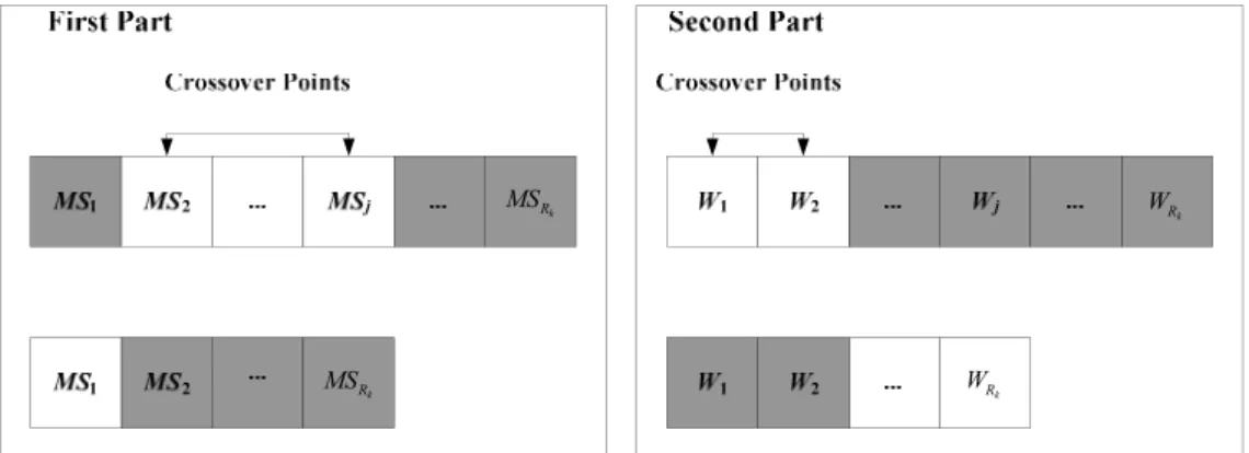
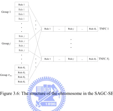
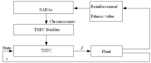
(11) List of Figures Figure 2.1: Structure of the TSK-type neuro-fuzzy controller. ................................................18 Figure 2.2: Reinforcement learning method.............................................................................20 Figure 2.3: Flow chart of the genetic algorithm. ......................................................................24 Figure 2.4: The roulette wheel selection. .................................................................................24 Figure 2.5: Crossover Operator. ...............................................................................................25 Figure 2.6: Mutation Operator. .................................................................................................25 Figure 2.7: Structure of a chromosome in a symbiotic evolution. ...........................................28 Figure 2.8: The flow chart of the symbiotic evolution. ............................................................29 Figure 3.1: Coding the adjustable parameters of a TNFC into a chromosome in the MVGA. 33 Figure 3.2: Coding the probability vector into the building blocks (BBs) in the MCGA. .......33 Figure 3.3: The flowchart of the parameter learning in the HEA.............................................34 HEA........................................ Figure 3.4: The variable two-part crossover operati operation in the HEA. ........................................39 ..................................... operation in the HEA. .........................................39 Figure 3.5: The variable two-part mutation operatio Figure 3.6: The structure of the chromosome in the SAGC-SE...............................................42 Figure 3.7: Coding the probability vector into the building blocks (BBs) in the TSSA. .........43 Figure 3.8: Coding a rule of a TNFC into a chromosome in SAGC-SE. .................................43 Figure 3.9: The learning process of SAGC-SE. .......................................................................44 Figure 3.10: Two-point crossover. ............................................................................................52 Figure 3.11: The learning process of the SAG-SEFA. .............................................................56 Figure 3.12: (a) Steps for constructing the FP-tree of sample transactions. (b) FP-tree of sampletransaction…………………………………………………………………….….62 Figure 4.1: Schematic diagram of the ISRL-SAEAs for the TNFC. ........................................73 Figure 4.2: Flowchart of the ISRL-SAEAs. .............................................................................74 Figure 4.3: Learning process of the ISRL. ...............................................................................76 ix.

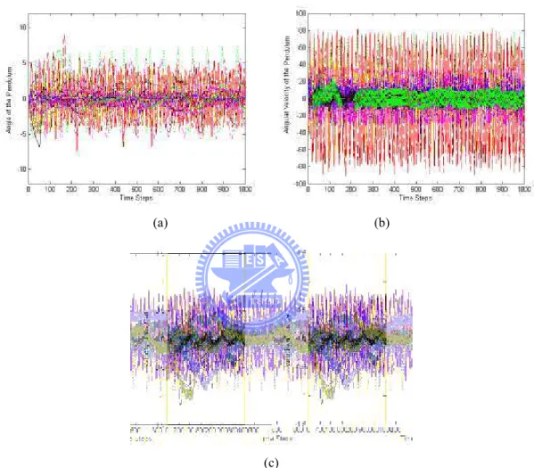
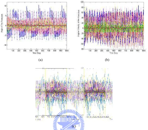
(12) Figure 5.1: The inverted pendulum control system.................................................................80 Figure 5.2: The learning curves of the ISRL-HEA. ................................................................85 Figure 5.3: The probability vectors of the ERS step in the ISRL-HEA. .................................85 Figure 5.4: Control results of the inverted pendulum control system using the ISRL-HEA in Example 1. (a) Angle of the pendulum. (b) Angular velocity of the pendulum. (c) Velocity of the cart...........................................................................................................86 Figure 5.5: Control results of the inverted pendulum control system using the R-SE in Example 1. (a) Angle of the pendulum. (b) Angular velocity of the pendulum. (c) Velocity of the cart...........................................................................................................87 Figure 5.6: Control results of the inverted pendulum control system using the R-GA in Example 1. (a) Angle of the pendulum. (b) Angular velocity of the pendulum. (d) cart.................................................................................. Velocity of the cart...........................................................................................................88 pendulu control system in Example 1. (a) Angle Figure 5.7: Control results of the inverted pendulum o the pendulum of ISRL-HEA. (c) of the pendulum of ISRL-HEA. (b) Angular velocity of Velocity of the cart of ISRL-HEA. (d) Angle of the pendulum of R-SE. (e) Angular velocity of the pendulum of R-SE. (f) Velocity of the cart of R-SE. (g) Angle of the pendulum of R-GA. (h) Angular velocity of the pendulum of R-GA. (i) Velocity of the cart of R-GA. ...................................................................................................................90 Figure 5. 8: Control results of the inverted pendulum control system using the SRL-HEA in Example 1. (a) Angle of the pendulum. (b) Angular velocity of the pendulum. (d) Velocity of the cart...........................................................................................................94 Figure 5. 9: The results of the probability vectors in the TSSA. .............................................97 Figure 5. 10: The learning curve of the SACG-SE..................................................................98 Figure 5. 11: Control results of the inverted pendulum control system using the ISRL-SACG-SE in Example 1 (first 1000 time). (a) Angle of the pendulum. (b) Angular velocity of the pendulum. (c) Velocity of the cart. ..........................................................98 x.

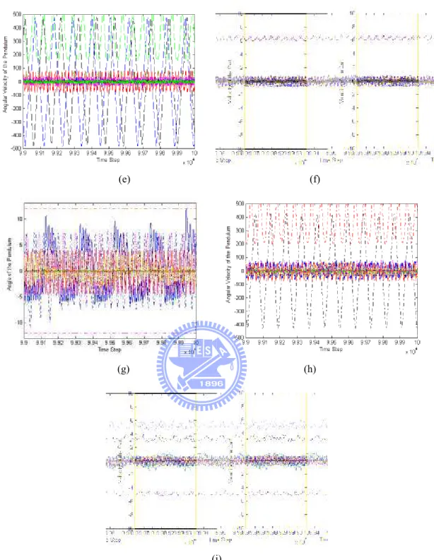
(13) Figure 5. 12: Control results of the inverted pendulum control system using the ISRL-SACG-SE in Example 1 (last 1000 time). (a) Angle of the pendulum. (b) Angular velocity of the pendulum. (c) Velocity of the cart. ..........................................................99 Figure 5. 13: The learning curve of the ISRL-SAG-SEFA. ..................................................104 Figure 5. 14: Control results of the inverted pendulum control system using the ISRL-SAG-SEFA in Example 1 (first 1000 time). (a) Angle of the pendulum. (b) Angular velocity of the pendulum. (c) Velocity of the cart. ..........................................105 Figure 5. 15: Control results of the inverted pendulum control system using the ISRL-SAG-SEFA in Example 1 (last 1000 time). (a) Angle of the pendulum. (b) Angular velocity of the pendulum. (c) Velocity of the cart. ........................................................106 Figure 5. 16: The tandem pendulum control system. ............................................................ 110 . Figure 5. 17: The learning curves of the ISRL-HEA. ........................................................... 114 pendulu control system using the ISRL-HEA. (a) Figure 5. 18: Control results of the tandem pendulum Angle of the first pendulum. (b) Angle of the second secon pendulum. (c) Angular velocity of the first pendulum. (d) Angular velocity of the second pendulum. ............................... 115 sec Figure 5. 19: Control results of the tandem pendulum control system using the R-SE. (a) Angle of the first pendulum. (b) Angle of the second pendulum. (c) Angular velocity of the first pendulum. (d) Angular velocity of the second pendulum. ............................... 116 Figure 5. 20: Control results of the tandem pendulum control system using the R-GA. (a) Angle of the first pendulum. (b) Angle of the second pendulum. (c) Angular velocity of the first pendulum. (d) Angular velocity of the second pendulum. ............................... 117 Figure 5. 21: Control results of the tandem pendulum control system. (a) Angle of the first pendulum of ISRL-HEA. (b) Angle of the second pendulum of ISRL-HEA. (c) Angular velocity of the first pendulum of ISRL-HEA. (d) Angular velocity of the second pendulum of ISRL-HEA. (e) Angle of the first pendulum of R-SE. (f) Angle of the second pendulum of R-SE. (g) Angular velocity of the first pendulum of R-SE. (h) xi.

(14) Angular velocity of the second pendulum of R-SE. (i) Angle of the first pendulum of R-GA. (j) Angle of the second pendulum of R-GA. (k) Angular velocity of the first pendulum of R-GA. (l) Angular velocity of the second pendulum of R-GA. ............... 119 Figure 5. 22: The learning curve of the SACG-SE................................................................122 Figure 5. 23: Control results of the tandem pendulum control system using the ISRL-SACG-SE (first 1000 time). (a) Angle of the first pendulum. (b) Angle of the second pendulum. (c) Angular velocity of the first pendulum. (d) Angular velocity of the second pendulum. ..........................................................................................................123 Figure 5. 24: Control results of the tandem pendulum control system using the ISRL-SACG-SE (last 1000 time). (a) Angle of the first pendulum. (b) Angle of the second pendulum. (c) Angular velocity of the first pendulum. (d) Angular velocity of the ...................................................................................... second pendulum. ..........................................................................................................123 .. Figure 5. 25: The learning curve of the SAG-SEFA. ............................................................127 pendulu Figure 5. 26: Control results of the tandem pendulum control system using the f ISRL-SAG-SEFA (first 1000 time). (a) Angle of the first pendulum. (b) Angle of the second pendulum. (c) Angular velocity of the first pendulum. (d) Angular velocity of the second pendulum. ..........................................................................................................127 Figure 5. 27: Control results of the tandem pendulum control system using the ISRL-SAG-SEFA (last 1000 time). (a) Angle of the first pendulum. (b) Angle of the second pendulum. (c) Angular velocity of the first pendulum. (d) Angular velocity of the second pendulum. ..........................................................................................................128. xii.

(15) Chapter 1 Introduction In real world application, many control problems are so complex that designing controllers by conventional means is either impractical or results in poor performance such as double link control system, inverted pendulum control system, tandem pendulum control system, water temperature control system, and ball and beam balance system, etc. Among them, mathematical models for designing controllers are needed. Inaccurate mathematical modeling of plants usually degrades the performance of the controllers, especially for nonlinear and complex problems. Moreover, even if the t neuro-fuzzy controller is adopted for avoiding the complex mathematical models, in real-world applications, precise training data real-w are usually difficult and expensive to obtain. For solving these problems, this dissertation controllers automatically by evolving improved provides a methodology for designing such controlle safe reinforcement learning (ISRL) via neuro-fuzzy controllers using self adaptive evolutionary algorithms (SAEAs). The introduction of this dissertation is introduced in this chapter. In Section 1.1, a motivation of this dissertation is discussed. The research purpose of this dissertation is introduced in Section 1.2. In Section 1.3, the approach of this dissertation is described. The overview of this dissertation is introduced in the final section.. 1.1 Motivation Neuro-fuzzy controllers ([1]-[14]) are capable of inferring complex nonlinear relationships between input and output variables. This property is important when the system 1.

(16) to be modeled is nonlinear. The key advantage of the neuro-fuzzy approach lies in the fact that it does not require a mathematical description of the system while modeling it. The system can perform the nonlinear mapping once the system parameters are trained based on a sequence of input and desired response pairs. The training of the parameters (parameter learning) is a problem in designing a neuro-fuzzy controller. Hence, techniques capable of training the system parameters and finding the global solution while optimizing the overall structure are needed. In this respect, genetic algorithms (GAs) appear to be better candidates. Among GAs, there are two major learning structures using for tuning the parameters of neuro-fuzzy controller: supervised learning ([2], [3], and [6]) and reinforcement learning ([15]-[21]). Among them, for some real-world applications, precise training data are usually difficult and expensive to obtain. For this reason, there has been a growing interest in rreinforcement learning algorithms for neural controller ([15]-[18]) or fuzzy design ([19]-[21]). For the reinforcement learning problems, training data are very rough and coarse and there aare only “evaluative” when compared with the “instructive” feedback in the supervised learning problem. In reinforcement learning, there is an agent which can choose which action gets the maximum reward in every state. The only feed back is the reward signal of success or failure. There are several evolutionary algorithms ([22]-[31]) which have been proposed to tune the parameters of the fuzzy controller. These algorithms may require one or more of the following problems: 1) it is difficult to know if it works with different conditions of the system or it can still controlled or nor in the letter time steps; 2) all the fuzzy rules are encoded into one chromosome; 3) the number of fuzzy rules has to be assigned in advance; 4) the population cannot evaluate each fuzzy rule locally. As mentioned above, improved safe reinforcement learning (ISRL) based self adaptive evolutionary algorithms (SAEAs) for neuro-fuzzy controller are proposed. The proposed 2.

(17) ISRL-SAEAs focus on not only the reinforcement learning but also the structure of the chromosomes in evolutionary algorithms. Therefore, in reinforcement learning, the architecture should consider not only how well and how soon the controller controls the system but also the stability analysis of the reinforcement learning. Moreover, in evolutionary algorithms, the number of fuzzy rules should be decided automatically and the population should evaluate each fuzzy rule locally.. 1.2 Review of previous works In recent years, a fuzzy system used for control problems has become a popular research topic because of classical control theory usually requires a mathematical model for designing controllers ([1]-[10]). Inaccurate mathematical modeling of plants usually degrades the performance of the controllers, especially for nonlinear and complex problems ([11]-[14]). A nonl fuzzy system consists of a set of fuzzy if-then rules. rul Conventionally, the selection of fuzzy if-then rules often relies on a substantial amount of heuristic observations to express the knowledge of proper strategies. Obviously, it is difficult for human experts to examine all the input-output data from a complex system to find proper rules for a fuzzy system. To cope with this difficulty, several approaches try to generate if-then rules from numerical data have been proposed ([2], [3], and [6]). These methods were developed for supervised learning; that is, the correct “target” output values are given for each input pattern to guide the network's learning. It is a powerful training technique that can be applied to networks. However, if the precise training data can be obtained easily, the supervised learning algorithm may be efficient in many applications. For some real-world applications, precise training data are usually difficult and expensive to obtain. For this reason, there has been a growing interest in reinforcement learning problems ([15]-[21]). For the reinforcement learning problems, training data are very rough and coarse and there are only “evaluative” when compared with. 3.

(18) the “instructive” feedback in the supervised learning problem. In the reinforcement learning, the well known algorithm is Barto and his colleagues’ actor-critic architecture ([17]), which consists of a control network and a critic network. However, the Barto’s architecture is complicated and is not easy to implement. About this, several researches proposed time-step reinforcement architecture to improve the Barto’s architecture ([18]-[20]). In time-step reinforcement architecture, the only available feedback is a reinforcement signal that notifies the model only when a failure occurs. An accumulator accumulates the number of time steps before a failure occurs. Even though time-step reinforcement architecture is easier to implement when compared with Barto’s architecture, it can only measure the number of time steps before a failure occurs; in other words, it only evaluates how long the controller works well instead of how soon the system can enter the desired state, which is also very important. Recent Recently, Perkins and Barto proposed a safe reinforcement learning based on Lyapunov function ddesign ([32]). Once the system’s Lyapunov-based manipulations on control laws, the Lyapunov function is identified, under Lyapunov-bas remain in a predefined desired set of states with architecture can drive the plant to reach and remai probability 1. Then, the time step for the plant entering the desired set of states can indicate the concept of how soon the system becomes stable. Therefore, one major part of this dissertation is identified. In learning algorithm, the most well known learning algorithm is back-propagation (BP) ([3], [6]-[8]). Since the steepest descent technique used in BP can minimize the error function, the algorithm may reach the local minima very fast and never find the global solution. In addition, the performance of BP training depends on the initial values of the system parameters, and for different network topologies one has to derive new mathematical expressions for each network layer. Recently, several evolutionary algorithms, such as the genetic algorithm (GA) ([22]), genetic programming ([23]), evolutionary programming ([24]), and evolution strategies ([25]), have grown into a popular researching area. They are parallel 4.

(19) and global search techniques. Because they simultaneously evaluate many points in the search space, they are more likely to converge toward the global solution. In recent years, there are several approaches try to use evolutionary algorithms to converge toward the global solutions. The one important field of these approaches is to use evolutionary algorithms for training fuzzy models ([26]-[28]). The evolutionary fuzzy model generates a fuzzy system automatically by incorporating evolutionary learning procedures. The well-known evolutionary algorithms are the genetic algorithms (GAs). Several genetic fuzzy models, that is, fuzzy models that are augmented by a learning process based on GAs, have been proposed ([26]-[28]). In [26], Karr applied GAs to design the membership functions of a fuzzy controller, with the fuzzy rule set assigned in advance. Carse et al. ([27]) used the genetic algorithm to evolve fuzzy rule-based controllers. Lin and Jou ([28]) proposed GA-based fuzzy reinforc reinforcement learning to control magnetic bearing systems. Recently, several improved evolutionary algorithms have been proposed. One catalogs is focus on modified the structure of the chromosomes ([29]-[44]). In such researches, the chromosomes in population represent partial solution or are with different length. In [29], Juang et al. proposed genetic reinforcement learning in the design of fuzzy controllers. The GA adopted in [29] was based upon traditional symbiotic evolution which, when applied to fuzzy controller design, complemented the local mapping property of a fuzzy rule. In [30], Bandyopadhyay et al. used the variable-length genetic algorithm (VGA) that allows for different lengths of chromosomes in a population. In [33], Ting et al. used multiobjective (MO) variable length genetic algorithm to solve the problem of placing wireless transmitters to meet particular objectives. As shown in [33], the authors used multiobjective (MO) variable length genetic algorithm for searching the optimal number, types, and positions of heterogeneous transmitters by considering coverage, cost, capacity, and overlap simultaneously. In [34], Saeidpour et al. used variable length genetic algorithm for fuzzy 5.

(20) controller design and used it for promotion voltage profile. In [35], Lin and Hsu proposed a reinforcement self-adaptive evolutionary algorithm with fuzzy system for solving control problems. As shown in [35], both the number of rules and the adjustment of parameters in the fuzzy system are designed concurrently by the proposed algorithm. The illustrative example was conducted to show the performance and applicability of the proposed algorithm. In [36], the Saha et al. proposed a differential evolution based fuzzy clustering for automatic clustering data set. The proposed algorithm has been used as a stochastic optimization tool. As shown in [36], the proposed algorithm performs better than others. In [37], Tang proposed a hierarchical genetic algorithm. The hierarchical genetic algorithm ([38]-[39]) enables the optimization of the fuzzy system design for a particular application. In [39], authors used a hierarchical genetic algorithm for solving the multilevel redundancy allocation problems. As shown in [39], the authors applied the HGA and a conventional GA separately for solving two multilevel series redund redundancy allocation optimization problems. The simulation results showed that the performance of the t HGA is superior to the conventional GA, because it does not depend on the use of vector coding and preserve the original design space. Gomez and Schmidhuber proposed lots of work to evaluate the solution locally ([40] and [41]). The proposed enforced sub-populations (ESP) used sub-populations of neurons for the fitness evaluation and overall control. As shown in [40] and [41], the sub-populations that use to evaluate the solution locally can obtain better performance compared to systems of only one population be used to evaluate the solution. In [42], Li and Miao proposed using ESP backpropagation (BP) neural network to the agent controllers in intelligent virtual environment (IVE). As shown in [42], the ESP was used to solve the task assignment problem of collaboration in an entertainment IVE platform. Juang [43] proposed the combination of online clustering and Q-value based GA for reinforcement fuzzy system (CQGAF) to simultaneously design the number of fuzzy rules 6.

(21) and free parameters in a fuzzy system. Lin and Xu ([44]) proposed a sequential search-based dynamic evolution (SSDE) to enable better chromosomes to be initially generated while better mutation points are determined for performing dynamic-mutation. Although the above evolutionary learning algorithms ([29]-[44]) improve the evolutionary learning algorithms through modifying the structure of chromosomes, these algorithms may have one or more of the following problems: 1) all the fuzzy rules are encoded into one chromosome; 2) the number of fuzzy rules has to be assigned in advance; and 3) the population cannot evaluate each fuzzy rule locally. About above problems, this dissertation focuses on not only the reinforcement learning but also the evolutionary algorithm. Therefore, in reinforcement learning, the architecture should consider how soon the system becomes stable. Moreover, in evolutionary algorithm, automa the numbers of fuzzy rules should be decided automatically and the population should evaluate each fuzzy rule locally.. 1.3 Research Purpose In this dissertation, improved safe reinforcement learning (ISRL) based self adaptive evolutionary algorithms (SAEAs) for neuro-fuzzy controller is proposed for improving not only the reinforcement signal designed but also evolutionary algorithms mentioned in Section 1.1. There are two parts in the proposed ISRL-SAEAs. In the first part, self adaptive evolutionary algorithms (SAEAs) are proposed to solve the following problems: 1) all the fuzzy rules are encoded into one chromosome; 2) the number of fuzzy rules has to be assigned in advance; and 3) the population cannot evaluate each fuzzy rule locally. In this dissertation, the proposed self adaptive evolutionary algorithms (SAEAs) consist of three different evolution methods to provide different ways to solve the above problems.. 7.

(22) First of all, the hybrid evolutionary algorithm (HEA) with a TSK-type neuro-fuzzy controller is proposed, the proposed HEA determines the number of fuzzy rules automatically and processes the variable-length chromosomes. The length of each individual denotes the total number of genes in that individual. The initial length of each individual may be different from each other, depending on the total number of rules encoded in it. Individuals with an equal number of rules constitute the same group. Thus, initially there are several groups in a population. For keeping the best group in every generation, the elite-based reproduction strategy (ERS) is proposed. In the ERS, the best group can be reproduced many times for each generation. The advantages of the proposed HEA are summarized as follows: 1) it determines the number of fuzzy rules and tunes the free parameters of the neuro-fuzzy controller in a highly autonomous way. Thus, users need not give it any a priori knowledge or even any initial information on these. 2) It is applicable to chromosomes of different lengths. 3) It does not require precise training data for setting the parameters parameters of the neuro-fuzzy controller. Although the proposed HEA can determine the number of fuzzy rules automatically, all the fuzzy rules are encoded into one chromosome. Therefore, partial solution cannot be Th evaluated independently in the population. The partial solutions can be characterized as specializations. The specialization property ensures diversity and prevents a population from converging to suboptimal solutions. A single partial solution cannot “take over” a population since it must correspond with other specializations. For solving this problem, the secondary algorithm of the SAEAs is proposed. In the secondary algorithm of the SAEAs, a self adaptive group cooperation based symbiotic evolution (SAGC-SE) is proposed not only for solving the problem that all the fuzzy rules are encoded into one chromosome but also for letting the population evaluate each fuzzy rule locally. Therefore, in the proposed SAGC-SE, each chromosome represents only one fuzzy rule and an n-rules TSK-type neuro-fuzzy controller is constructed by selecting and combining n chromosomes from several groups. The SAGC-SE, which promotes both cooperation and specialization, ensures diversity and 8.

(23) prevents a population from converging to suboptimal solutions. In SAGC-SE, there are several groups in the population. Each group formed by a set of chromosomes represents a fuzzy rule. The proposed SAGC-SE consists of structure learning and parameter learning. In structure learning, as well as HEA, the SAGC-SE determines the number of fuzzy rules automatically and processes the variable length of a combination of chromosomes. In parameter learning, to let the well-performing groups of individuals for cooperating to generate better generation, an elite-based compensatory of crossover strategy (ECCS) is proposed. In the ECCS, each group will cooperate to perform the crossover steps. Therefore, the better chromosomes of each group will be selected to perform crossover in the next generation. The advantages of the proposed SAGC-SE are summarized as follows: 1) the proposed automa SAGC-SE determines the number of fuzzy rules automatically. 2) The SAGC-SE uses l group-based population to evaluate the fuzzy rule locally. 3) The SAGC-SE uses the ECCS to allow the better solutions from different groups to cooperate for generating better solutions in the next generation. The SAGC-SE can solve the problem of the HEA that all the fuzzy rules are encoded into one chromosome. Moreover the SAGC-SE evaluates each fuzzy rule locally for improving the local consideration of the population. However, in the SAGC-SE, how to select groups for constructing the complete solution is a major problem. Therefore, for determining the number of fuzzy rules automatically, the SAGC-SE selects different number of groups to construct complete solution. In this way, the SAGC-SE selects groups randomly. It’s obvious that the performance of the SAGC-SE dependents on the method of selecting groups. For solving this problem, in the third algorithm of the SAEAs, a self adaptive groups based symbiotic evolution using FP-growth algorithm (SAG-SEFA) is proposed. As well as SAGC-SE, the SAG-SEFA consists of structure learning and parameter learning. In structure learning, as well as the SAGC-SE, the proposed SAG-SEFA determines 9.

(24) the number of fuzzy rules automatically and processes the variable combination of chromosomes. In parameter learning, although the proposed SAG-SEFA can determine the suitable number of rules, there still has a problem in which how to select the suitable groups from many groups (named candidate groups in this paper) in SAG-SEFA to construct TSK-type neuro-fuzzy controllers with different numbers of rules. Moreover, in consideration of making the well-performing groups of individuals cooperate for generating better generation, there is also a problem in which how to select suitable groups used to select individuals for cooperating to generate better generation. Regarding this, the goals of parameter learning in SAG-SEFA are used to determine which groups of chromosomes should be selected to construct TSK-type neuro-fuzzy networks with different numbers of rules and which groups should be selected for cooperating to generate better generation. Recently, data mining has become a popular research topic ([45]-[48]). Data mining is a method of mining information from a database. The ddatabase called “transactions”. Data mining can be regarded as a new way of performing ddata analysis. One goal of data mining is to find association rules among sets of items that occur frequently in transactions. To achieve this goal, several methods have been proposed ([49]-[54]). In [49], the authors proposed a mining method which ascertains large sets of items to find the association rules in transactions. Hang et al. ([50]) proposed frequent pattern growth (FP-growth) to mine frequent patterns without candidate generations. In Hang’s work, items that occur more frequently will have better chances of sharing information than items that occur less frequently. In [51], an algorithm of data mining for transaction data with quantitative values was proposed. In [51], each quantitative item was translated to a fuzzy set and the authors used these fuzzy sets to find fuzzy rules. Wu et al. ([52]) proposed a data mining method based on GA algorithm that efficiently improves the traditional GA by using analysis and confidence parameters. In [53], authors proposed a hybrid model using rough sets and genetic algorithms for fast and efficient improving answering data mining query which involves a random search over large databases. 10.

(25) As shown in [53], authors proposed select, aggregate and classification based data mining queries to implement a hybrid model. The performance of the proposed algorithm is analyzed for both execution time and classification accuracy and the results obtained are good. In [54], Dai and Zhang proposed an association rules mining in novel genetic algorithm. The genetic algorithm in [54] are using for discovering association rules. As shown in [54], the proposed algorithm avoids generating impossible candidates, and it is more efficient than traditional ones. Since data mining can successfully find information from large sets of items, it is useful to achieve goals of parameter learning in SAG-SEFA. Therefore, the data-mining method called FP-growth algorithm is adopted since the FP-growth algorithm can find items that occur frequently in transactions without candidate generations. After the parameter learning populati can search for a better solution from with FP-growth algorithm is performed, the population an explore other combinations of the combination of individuals that perform well and individuals. Moreover, suitable groups will cooperate coopera to perform the crossover steps. Therefore, the better chromosomes of suitable group will be selected to perform crossover in the next generation. When compared with SAGC-SE, the proposed SAG-SEFA not only selects the suitable groups form candidate groups to perform selection steps but also allows the better solutions from different groups to cooperate for generating better solutions in the next generation. The second part of the proposed ISRL-SAEAs is an improved safe reinforcement learning (ISRL). In the ISRL, the feedback takes the form of an accumulator. The accumulator determines by two different strategies (judgment and evaluation). The judgment strategy determines the reinforcement signal when the plant fails entering a predefined goal set and the evaluation strategy applies under the condition that the plant enters the goal set. Moreover the safe reinforcement learning [32] is considered in ISRL. The key of the ISRL is using an accumulator determined by two different strategies as the fitness function of the SAEAs. It 11.

(26) will be observed that the advantage of the proposed ISRL is that it can meet global optimization capability.. 1.4 Approach To demonstrate the performance of the ISRL-SAEAs for temporal problems, this dissertation presents two examples and performance contrasts with some other models. In the first example, the inverted pendulum control system is adopted to evaluate the performance of the proposed ISRL-SAEAs of this dissertation. This problem is often used as an example of inherently unstable and dynamic systems to demonstrate both modern and classical control techniques ([55]-[57]) or the reinforcement learning schemes ([15]-[21]), and is now used as a control benchmark. In the second example, the tandem pendulum control system is adopted to evaluate the dissertation. Since the task of an inverted performance of the proposed method of this disserta solutions quickly through random search, in this pendulum control system is too easy to find solutio example, a variety of extensions to an inverted pendulum control system have been suggested. The most challenging extension of an inverted pendulum control system ([58]-[60]) is a tandem pendulum control system, where two pendulums of different length must be balanced synchronously.. 1.5 Overview of Dissertation This dissertation consists of six chapters. In Chapter 1, the introduction consists of motivation, review of previous works, research goal, approach, and overview of this dissertation. In Chapter 2, the foundation for the four components of the proposed ISRL-SAEAs by providing background material on neuro-fuzzy controller, reinforcement learning, Lyapunov 12.

(27) stability, and evolutionary algorithm. In Chapter 3, the first part of the proposed ISRL-SAEAs is self adaptive evolution algorithms (SAEAs). The SAEAs consist of a hybrid evolutionary algorithm (HEA), self adaptive groups’ cooperation based symbiotic evolution (SAGC-SE), and self adaptive groups based symbiotic evolution using FP-growth algorithm (SAG-SEFA). These three algorithms are introduced in this chapter. In Chapter 4, the second part of the proposed ISRL-SAEAs is the improved safe reinforcement learning (ISRL). The ISRL consists of novel reinforcement signal designed and Lyapunov stability analysis. Both of these two components will be introduced in this chapter. In Chapter 5, to demonstrate the performance of the ISRL-SAEAs for temporal problems, two examples and performance contrasts with some other models are presented. inverte pendulum control system and tandem The examples of this chapter consist of the inverted pendulum control system. direc In Chapter 6, the contributions and outlines some promising directions for future research are discussed.. 13.

(28) Chapter 2 Foundations The background material and literature review that relates to the major components of the research purpose outlined above (neuro-fuzzy controller, reinforcement learning, Lyapunov stability, and evolutionary algorithm) are introduced in this chapter. The concept of neuro-fuzzy controller is discussed in the first section. The reinforcement learning schema is introduced in Section 2.2. In Section 2.3, the Lyapunov stability that the improved safe reinforcement learning (ISRL) is discussed. The final section focuses on genetic algorithm, cooperative coevolution, and symbiotic evolution, the t method on which the proposed self adaptive evolutionary algorithms (SAEAs) are based.. 2.1 Neuro-Fuzzy Controller Neuro-fuzzy modeling has been known as a powerful tool ([1]-[14]) which can facilitate the effective development of models by combining information from different sources, such as empirical models, heuristics and data. Neuro-fuzzy models describe systems by means of fuzzy if–then rules represented in a network structure, to which learning algorithms known from the area of artificial neural networks can be applied. A neuro-fuzzy controller is a knowledge-based system characterized by a set of rules, which model the relationship among control input and output. The reasoning process is defined by means of the employed aggregation operators, the fuzzy connectives and the inference method. The fuzzy knowledge base contains the definition of fuzzy sets stored in the fuzzy database and a collection of fuzzy rules, which constitute the fuzzy rule base. Fuzzy 14.

(29) rules are defined by their antecedents and consequents, which relate an observed input state to a desired output. Two typical types of neuro-fuzzy controllers are Mamdani-type and TSK-type neuro-fuzzy controllers. For Mamdani-type neuro-fuzzy controllers ([1]), the minimum fuzzy implication is used in fuzzy reasoning. The neuro-fuzzy controllers employ the inference method proposed by Mamdani in which the consequence parts are defined by fuzzy sets. A Mamdani-type fuzzy rule has the form: IF x1 is A1j (m1j , σ1j ) and x2 is A2j(m2j , σ2j )…and xn is Anj (mnj , σnj) THEN y’ is Bj (mj ,σj ). (2.1). where mij , and σ ij represent a Gaussian membership function with mean and deviation with ith dimension and jth rule node. The consequences Bj of jth rule is aggregated into one fuzzy. defuzzification, which set for the output variable y’. The crisp output is obtained through defuzzificat calculates the centroid of the output fuzzy set. Besides the more common fuzzy inference method prop proposed by Mamdani, Takagi, Sugeno and Kang introduced a modified inference scheme ([5]). The first two parts of the fuzzy inference process, fuzzifier the inputs and applying the fuzzy operator are exactly the same. A Takagi-Sugeno-Kang (TSK) type fuzzy model employs different implication and aggregation methods than the standard Mamdani’s type. For TSK-type neuro-fuzzy controllers ([5]), the consequence of each rule is a function input variable. The general adopted function is a linear combination of input variables plus a constant term. A TSK-type fuzzy rule has the form: IF x1 is A1j (m1j , σ1j ) and x2 is A2j(m2j , σ2j )…and xn is Anj (mnj , σnj ) THEN y’=w0j+w1jx1+…+wnjxn. (2.2). where w0j represents the first parameter of a linear combination of input variables with jth rule node and wij represents the ith parameter of a linear combination of ith input variable. Since. 15.

(30) the consequence of a rule is crisp, the defuzzification step becomes obsolete in the TSK inference scheme. Instead, the model output is computed as the weighted average of the crisp rule outputs, which is computationally less expensive then calculating the center of gravity. Recently, there are many researchers ([5], [35], and [44]) to show that using a TSK-type neuro-fuzzy controller achieves superior performance in network size and learning accuracy than that of Mamdani-type neuro-fuzzy controllers. According to this reason, in this dissertation, a TSK-type neuro-fuzzy controller (TNFC) is adopted to perform various dynamic problems. Therefore, the proposed SAEAs are used to tune free parameters of a TNFC. The structure of a TNFC is shown in Fig. 2.1, where n and R are, respectively, the number of input dimensions and the number of rules. It is a five-layer network structure. The functions of the nodes in each layer are described as follows: Layer 1 (Input Node): No function is performed in this layer. The node on only transmits input values to layer 2. u i(1) = xi ,. (2.3). where u i(k ) denotes the ith node’s input in the kth layer and xi denotes ith input dimension.. Layer 2 (Membership Function Node): Nodes in this layer correspond to one linguistic label of the input variables in layer1; that is, the membership value specifying the degree to which an input value belongs to a fuzzy set ([3]-[4]) is calculated in this layer. In this dissertation, the Gaussian membership function is adopted in this layer. Therefore, for an external input xi , the following Gaussian membership function is used:. u. ( 2) ij. [.  u (1) − m i ij = exp − 2  σ ij . ]. 2.    . (2.4). where mij and σ ij are, respectively, the center and the width of the Gaussian membership 16.

(31) function of the jth term of the ith input variable xi .. Layer 3 (Rule Node): The output of each node in this layer is determined by the fuzzy AND operation. Here, the product operation is utilized to determine the firing strength of each rule. The function of each rule is uj. ( 3). = ∏ u ij( 2). (2.5). i. Layer 4 (Consequent Node): Nodes in this layer are called consequent nodes. The input to a node in layer 4 is the output derived from layer 3, and the other inputs are the input variables from layer 1 as depicted in Fig. 2.1. The function of a node in this layer is n. u (j4) = u (j3) ( w0 j + ∑ wij xi ). (2.6). i =1. where the summation is over all the inputs and where wij are the corresponding parameters of the consequent part.. Layer 5 (Output Node): Each node in this layer corresponds to single outpu output variable. The node integrates all the actions recommended by layers laye 3 and 4 and acts as a defuzzifier with R. R. ∑ u (j4) y = u (5) =. j =1. =. R. ∑u. n. ∑ u (j3) ( w0 j + ∑ wij xi ). ( 3) j. j =1. j =1. i =1. R. ∑u j =1. where R is the number of fuzzy rule.. 17. ( 3) j. (2.7).

(32) ̌. Layer 5 (Output nodes). Ξ. Layer 4 (Consequent nodes). n. w01 + ∑ wi1 xi i =1. n. n. w02 + ∑wi 2 xi. w03 + ∑wi3 xi. i =1. i =1. Ξ. Layer 3 ( rule nodes). Ξ. Layer 2 (membership function nodes). Ξ. Layer 1 (Input nodes). ̋˄. ̋˅. Figure 2. 1: Structure of the TSK-type neuro-fuzzy controller.. 2.2 Reinforcement Learning Unlike the supervised learning problem, in which th the correct “target” output values are given for each input pattern, the reinforcement learning problem has only very simple “evaluative” or “critical” information, rather than “instructive” information. Reinforcement learning algorithm is proposed for determining a sequence of decisions to maximize a reinforcement signal. At each time step, the agent in state st ∈ S , chooses an action a t ∈ A that transfers the environment to the state st +1 and returns a numerical reward, rt , to the agent. To lack of knowledge of how to solve the problem, the agent should explore the environment by trial-and-error learning strategy. Unlike supervised learning, the desired output in each state is not known in advance in reinforcement learning. In such trial-and-error learning strategy, an action performs well in the current states may perform badly in the future states, and vice versa. The well-known learning methods for solving control problems are dynamic 18.

(33) programming ([61]). These methods are similarly to the reinforcement learning ([62]). The necessary component of reinforcement learning methods is shown in Fig. 2.2. The agent consists of a value function and a strategy. The value function represents how much reward can be expected from each state if the best known strategy is performed. The strategy represents how to choose suitable actions from the value function to environment. As shown in Fig. 2.2, at time step t , the agent selects an action a t . The action is applied to the environment, causing a state transition from st to st +1 , and a reward rt is received. The goal of a reinforcement learning method is to find the optimal value function for a given environment. There are several reinforcement learning algorithms such as the Q-learning ([63]-[64]) and Sarsa ([65]) algorithms are proposed for computing the value function. These methods are developed based on the temporal difference learning algorithm. In the temporal difference learning method, the value function of each state ((V V( st )) is updated using the value function (V( of the next state (V( st +1 )). The value function of each state is shown as follows. fo V ( st ) = V ( s t ) + α [rt + λV ( s t +1 ) − V ( s t )],. (2.8). where V( st ) increases by the reward rt plus the difference between the next state λV ( s t +1 ) and V( st ); α is the learning rate between 0 to 1; and λ is the discount factor between 0 to 1.. 19.

(34) Figure 2. 2: Reinforcement learning method.. In early research, these reinforcement learning algorithms were proposed in simple environments.. Recently,. the. reinforcement. learning. algorithms. focus. on. larger,. high-dimensional environments. These reinforcement learning algorithms are developed base fu on the neural networks ([66]-[67]), radial basis functions ([68]), and neuro-fuzzy network ([18]-[20]). More recently, there are several researches proposed time-step reinforcement architectures to provide an easier way to implement the reinforcement learning architecture when compared with temporal difference learning architectures ([18]-[20]). In time-step reinforcement architecture, the only available feedback is a reinforcement signal that notifies the model only when a failure occurs. An accumulator accumulates the number of time steps before a failure occurs. The goal of the time-step reinforcement method is to maximize the value function V. The fitness function is defined by: V =TIME-STEP. (2.9). where TIME-STEP represents how long the experiment is still a “success”. Equation 2.9 reflects the fact that long-time steps before a failure occurs means the controller can control. 20.

(35) the plat well. For example, in evolutionary algorithm, Eq. 2.9 reflects the fact that long-time steps before a failure occurs means higher fitness of the evolutionary algorithm.. 2.3 Lyapunov Stability Consider a following system: xɺ = f (x). (2.10). where f : D → R n represents a locally Lipschitz that maps from an open set D ⊂ R n into R n . Suppose that x = 0 is an equilibrium point for Eq. 2.10; that is, f (0) = 0 . According to [69], we have the following definition of stability Definition 2.3.1: 1. Stable, if ∃δ (ε ) > 0, for ∀ε > 0 , such that. x(0) < δ ⇒ x(t ) < ε , ∀t ≥ 0. (2.11). exists some γ > 0 such that 2. Asymptotically stable, if it is stable and there ex. x(0) < γ ⇒ lim x(t ) = 0 t →∞. (2.12). 3. Globally asymptotically stable, if it is asymptotically stable and there exists. lim x(t ) = 0 holds for all x(0) . t →∞. 4. Unstable, if not stable. The Lyapunov stability theorems ([69]) are introduced as follows. Theorem 2.3.1 ([69]): Suppose x = 0 is an equilibrium point of Eq. 2.10 and D ⊂ R n is an open set containing x = 0 . Let V : D → R to be a continuously differentiable function as following V (0) = 0 and V ( x) > 0 in D \ {0} . According to Eq. 2.13, the following equations hold: 1. If. Vɺ ( x) ≤ 0 in D ,then x = 0 is stable, where Vɺ ( x) is defined by. 21. (2.13).

(36) ∂V Vɺ ( x) = ( f ( x)) . ∂x. (2.14). 2. If D = R n , Vɺ ( x) < 0 in D \ {0} , and V (x) is radially unbounded. An equilibrium point x = 0 is globally asymptotically stable, when x → ∞ and V (x) → ∞ . 3. If Vɺ ( x) < 0 in D \ {0} , then x = 0 is asymptotically stable. In reinforcement learning, the most well-known algorithm is Barto and his colleagues’ actor-critic architecture ([17]), which consists of a control network and a critic network. However, Barto’s architecture is complicated and is not easy to implement. Therefore, there are several researches proposed time-step reinforcement architectures to improve Barto’s architecture ([18]-[20]). In time-step reinforcement architecture, the only available feedback is a reinforcement signal that notifies the model only when a failure occurs. An accumulator failure occurs. Even though the time-step accumulates the number of time steps before a failu reinforcement architecture is easier to implement w when compared with Barto’s architecture, it failure occurs; in other words, it only only measures the number of time steps before a fai instead of how soon the system can enter the evaluates how long the controller works well instea desired state, which is also very important. In [32], Perkins and Barto proposed safe reinforcement learning based on Lyapunov function design. Once the system’s Lyapunov function is identified, under Lyapunov-based manipulations on control laws, the architecture can drive the system to reach and remain in a predefined desired state with probability 1. Then, the time step for the system entering the desired state can indicate the concept of how soon the system becomes stable. In this dissertation, the Lyapunov stability theorem is used to design the reinforcement signal; therefore, the improved safe reinforcement learning (ISRL) is based on the Lyapunov stability theorem. The details of the ISRL can be found in Chapter 4.. 22.

(37) 2.4 Evolution Learning In this section, the foundations of evolutionary algorithm are introduced. This section focuses on genetic algorithm, cooperative coevolution and symbiotic evolution, the methods on which the proposed self adaptive evolutionary algorithms (SAEAs) are based.. 2.4.1 Genetic algorithm Genetic algorithms (GAs) ([22]) are search algorithms inspired by the mechanics of natural selection, genetics, and evolution. It is widely accepted that the evolution of living beings is a process that operates on chromosome-organic devices for encoding the structure of living beings. The flowchart of the learning process is shown in Fig. 2.3, where Nc is the size of population, G denote Gth generation. The learning process of the GAs involves three major Repro steps: reproduction, crossover, and mutation. Reproduction ([70]-[72]) is a process in which fi individual strings are copied according to their fitness value. This operator is an artificial version of neural selection. In GAs, a high fitness value denotes a good fit. In the reproduction s step, the well-known method is the roulette-wheel selection method ([72]) (see Fig.2.4). In Fig.2.4, the intermediate population is P’, which is generated from identical copies of a chromosome sampled by spinning the roulette wheel a sufficient number of times.. 23.

(38) Figure 2. 3: Flowchart of the genetic algorithm.. C1. C1. P (C2 ) = 0.15. C2. P (C1 ) = 0.4. C1. P (C3 ) = 0.2 C3. C4. C4. C3. P (C4 ) = 0.25. Figure 2. 4: The roulette wheel selection.. In crossover step ([73]-[77]), although reproduction step directs the search toward the best existing individuals, it cannot create any new individuals. In nature, an offspring has two parents and inherits genes from both. The main operator working on the parents is the crossover operator, the operation of which occurred for a selected pair with a crossover rate. Figure 2.5 illustrates how the crossover works. Crossover produces two offspring from their parents by exchanging chromosomal genes on either side of a crossover point generated randomly. 24.

(39) Figure 2.5: Crossover operator.. In mutation step ([78]-[84]), although the reproduction and crossover would produce many new strings, they do not introduce any new information to the population at the site of an individual. Mutation can randomly alter the allele of a gene. The operation is occurred with a mutation rate. Figure 2.6 illustrates how the mutation works. When an offspring is mutated, one of its genes selected randomly is changed to a new value.. Figure 2.6: Mutation operator.. Since GAs search many points in the space simultaneously, they have less chance to reach the local minima than single solution methods. The advantages of GAs are (1) some individuals have a better chance to come close to the global optima solution, and (2) the genetic operators allow the GA to search optima solution. According to above reasons, GAs are suitable for searching the parameters space of neuro-fuzzy controller. For solving the problem that a neuro-fuzzy controller which performs gradient-descent based learning algorithms may reach the local minima very fast but never find the global solution, the GAs sample the parameters space of neuro-fuzzy controllers and recombine those that perform best on the control problem. 25.

(40) 2.4.2 Cooperative Coevolution In natural evolution, individuals may compete and/or cooperate with each other for resources and survival. The fitness of each individual may changes each generation. The reason is that individuals compete and/or cooperate with other individuals in the environment. About this phenomenon, recently, many researches try to propose coevolutionary algorithms to improve the traditional evolutionary algorithm. Most coevolutionary algorithms focus on competition between individuals in the population ([85]-[87]). Therefore, individuals generate stronger and stronger strategies to defeat others in every generation. Another kind of coevolutionary algorithms is proposed to improve cooperation of GAs. Cooperative coevolution is proposed for reducing the difficult problems through modularization ([88]). Therefore, in cooperative coevolutionary algorithms, the individuals solut represent only partial solutions. The partial solutions are evolved by evaluating their t performance to complete solutions and recombining the partial solutions with well coevo performance to solve the problem. Cooperative coevolution algorithms can improve the performance of traditional evolution by dividing the problem into several small problems. In [89], Holland and Reitman proposed cooperative coevolution algorithms to apply in classifier systems. The fitness value is assigned to each individual on how well it cooperates with others. This approach is implemented by a neural network. Recently, there are several researches try to use coevolution algorithms to radial basis functions ([90]-[93]). In [94], the authors proposed a cooperative coevolutionary GA that each individual is evaluated independently on its own population. More recently, several researches try to propose algorithms to combine cooperative coevolution with neural networks ([95]-[96]) and neuro-fuzzy controller ([29], [31], and [44]) to improve the performance. The approach called symbiotic evolution will be introduced in next section.. 26.

(41) 2.4.3 Symbiotic Evolution In this section, an approach of cooperative coevolution is introduced. Therefore, the symbiotic evolution is discussed. The idea of symbiotic evolution was first proposed in an implicit fitness sharing algorithm that was used in an immune system model ([97]). The authors developed artificial antibodies to identify artificial antigens. Because each antibody can match only one antigen, a different population of antibodies was required to effectively defend against a variety of antigens. Unlike traditional GAs that use each individual in a population as a full solution to a problem, symbiotic evolution assumes that each individual in a population represents only a partial solution to a problem; complete solutions combine several individuals in the population. In a normal evolution algorithm, a single individual is responsible for the overall performance, with a fitness value assigned to that individual according to its performance. In symbiotic evolution, the fitness of an individual (a partial solution) is calculated by summing up the fitness values of all possible combinations of that individual with other current individuals (partial solutions) and dividing the sum by the total number of combinations. As shown in [29], [31], [44], and [95]-[96], partial solutions can be characterized as specializations. The specialization property ensures diversity, which prevents a population from converging to suboptimal solutions. A single partial solution cannot “take over” a population since there must be other specializations present. Unlike the standard evolutionary approach, which always causes a given population to converge, hopefully at the global optimum, but often at a local one, the symbiotic evolution finds solutions in different, unconverted populations ([29], [31], [44], and [95]-[96]). The basic idea of symbiotic evolution is that an individual (i.e., a chromosome) is used to represent a partial solution. A complete solution is formed when several individuals,. 27.

(42) which are randomly selected from a population, are combined. With the fitness assignment performed by symbiotic evolution, and with the local property of a fuzzy rule, symbiotic evolution and the fuzzy system design can complement each other. If a normal GA evolution scheme is adopted, only the overall performance of the complete solution is known, not the performance of each partial solution. The best method to replace the unsuitable partial solutions that degrade the overall performance of a fuzzy system is to use crossover operations, followed by observing the performance of the offspring. The structure of the symbiotic evolution is shown in Fig. 2.7, where N is the number of complete solutions the symbiotic evolution will select individuals to form. The complete solution is constructed by selecting the individuals from a population. The learning flowchart is shown in Fig. 2.8, where Nc is the size of population, and G denotes Gth dif generation. Compare with genetic algorithm, the difference of symbiotic evolution is ( selecting individuals to form a complete solution (selection step) and to evaluate the performance of each individual (fitness assignments step).. Figure 2.7: Structure of a chromosome in a symbiotic evolution.. 28.