R E S E A R C H F E A T U R E
PROPOSED NAVIGATION PROTOCOL
We based our protocol on the temporally ordered routing algorithm2for mobile ad hoc networks. TORA
assigns mobile nodes temporally ordered sequence num-bers to support multipath routing from a source to a specific destination node. The algorithm expresses the sequence number as a quintuple.
To handle mobility, TORA adopts a link-reversal pro-cedure when hosts lose their outgoing paths. TORA’s multipath routing concept fits well with the requirements of emergency navigation services.
However, we can’t directly apply TORA to our envi-ronment for several reasons:
• Expressing a node’s weight as a quintuple can be too costly for sensors with weak communication capa-bility (for example, typical mote packets are only 29 bytes).
• TORA looks for shorter and multipath routes, whereas our navigation service looks for safer, but not necessarily shorter, escape paths.
• The considerations for users in hazardous and non-hazardous regions differ. Our navigation service is essentially an all-to-many routing (from all locations to one or multiple exits), and emergency locations disturb the discovery of safe paths.
We consider a sensor network deployed in a 2D indoor environment. Each sensor knows its own loca-tion in the 2D plane. By overhearing wireless signals, a
In an emergency, wireless network sensors combined with a navigation algorithm
could help safely guide people to a building exit while helping them avoid
hazardous areas.
Yu-Chee Tseng, Meng-Shiuan Pan, and Yuen-Yung Tsai
National Chiao Tung UniversityT
he rapid progress of wireless communications and embedded microelectromechanical systems technologies has made wireless sensor networks possible. WSNs typically need to configure themselves automatically and support ad hoc routing. Recent research efforts have focused on vari-ous WSN features, including power management, rout-ing and transportation, self-organization, deployment, coverage, and localization.WSN design is generally application driven—that is, a particular application’s requirements will determine how the network behaves. Current WSN projects include the Great Duck Island’s habitat-monitoring application (www.greatduckisland.net/index.php); the FireBug project (http://firebug.sourceforge.net), which uses wireless sensors with the Global Positioning System to monitor wildfires; and mobile object tracking.1
As the “Related Work in Emergency Navigation” side-bar describes, previous navigation applications weren’t designed with emergency applications in mind. In emer-gency applications, such as fire rescues, a safe escape path is more critical than factors such as energy consumption.
We propose a distributed navigation algorithm for emergency situations. At normal time, sensors monitor the environment. When the sensors detect emergency events, our protocol quickly separates hazardous areas from safe areas, and the sensors establish escape paths. Simulation and implementation results show that our scheme achieves navigation safety and quick conver-gence of the navigation directions.
Wireless Sensor Networks
for Emergency Navigation
sensor can form wireless links with its neighbors. Depending on how the plane is partitioned, a sensor could form navigation links with its neighbors. (Because of radio’s penetration capacity, a wireless link doesn’t necessarily imply a navigation link.)
We therefore manually define navigation links dur-ing deployment. From these links, we construct a navigation graph. In the following discussion, all oper-ations refer to the navigation graph, although the underlying message exchange is through wireless links. Our design emphasizes correctness in discovering escape paths even if users must pass hazardous areas. We divide the algorithm into two phases: initialization and navigation.
Initialization phase
In the initialization phase, we assign each sensor an altitude according to its hop distance to the nearest exit. We assign sensors near the exits smaller altitudes, and sensors farther from the exits higher altitudes. The escape paths are along sensors with higher altitudes to those with lower attitudes.
To compute sensors’ initial altitude, exit sensors broadcast initial packets to start the initialization phase. An initial packet consists of three fields: sender ID, exit sensor ID, and hop count. In an exit sensor broadcast, the hop count field is set to zero.
When a sensor receives an initial packet, it increments the hop count by one and accepts this value as its initial
alti-In previous work using an algorithm to guide a robot to a goal,1sensor nodes act as signposts for the robot to follow.
Each sensor determines the direction in which the robot should move by computing a probability value for each of its neighbors. A neighbor with a higher probability is closer to the goal.
Qun Li, Michael DeRosa, and Daniela Rus assumed that multiple emergency points (or obstacles) and one exit exist in the environment.2Their goal was to find a navigation path
from each sensor to the exit without passing any obstacles. They designed their algorithms using the artificial potential
fields concept.The exit generates an attractive potential,
pulling sensors to the exit, while each obstacle generates a repulsive potential, pushing sensors away from it. Each sen-sor calculates its potential value and tries to find a naviga-tion path with the least total potential value. Other researchers have applied this concept to other application
scenarios, such as robot navigation and distributed search and rescue.3
Although Li and his colleagues’ algorithm can find a shorter and safer path from each sensor to the exit, it has several drawbacks.
First, it can incur high message overheads. Because the algorithm constructs navigation directions from the exit to other sensors, a minor change of potential in a sensor near the exit can cause many other sensors to recompute their potentials, causing many message exchanges and even delays in making the navigation decision.
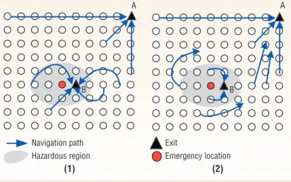
Second, the algorithm has no concept of hazardous regions.With shortest-path routing, the algorithm could determine a path that is very close to the emergency loca-tion. Consider Figure A1, in which there are two exits,A and B. When a sensor detects an emergency, the algorithm could direct some users to B, making them pass through the
hazardous region. Guiding users as in Figure A2 is more desirable because the algorithm only directs users inside the hazardous region to exit B.
References
1. M.A. Batalin, G.S. Sukhatme, and M. Hattig, “Mobile Robot Navigation Using a Sensor Net-work,” Proc. IEEE Int’l Conf. Robotics and
Automa-tion, IEEE Press, 2004, pp. 636-642.
2. P. Corke, R. Peterson, and D. Rus,“Networked Robots: Flying Robot Navigation Using a Sen-sor Net,” Proc. Int’l Symp. Robotics Research (ISRR), Springer Tracts on Advanced Robotics (STAR). Springer-Verlag, 2003.
3. Q. Li, M. DeRosa, and D. Rus,“Distributed Algorithm for Guiding Navigation across a Sensor Network,” Proc.ACM Int’l Symp.
Mobile Ad Hoc Networking and Computing
(MobiHOC),ACM Press, 2003, pp. 313-325. A A B B Navigation path Hazardous region Exit Emergency location (1) (2)
Figure A. Navigation scenarios in which the hazardous region is defined as two hops from the emergency site. (1) Users are directed to an exit in a hazardous region, even though another exit exists. (2) Only users already in the hazardous region are directed to exit B.
tude unless it has a smaller altitude. It then rebroadcasts the initial packet with the updated hop count. The initial-ization phase is complete when each sensor has an altitude.
Exit sensors periodically restart the initialization phase to adjust for possible topology changes. In this process, each sensor keeps a neighbor table, in which each entry is of the format <neighbor ID, is_exit, altitude> to track its neighbors’ status.
Navigation phase
The navigation phase begins when the system detects an emergency event. The goal is for each sensor to choose the neighbor with the smallest altitude as its escape direction.
We use the following notations:
• D is a constant such that any sensor whose distance to any emergency location is less than or equal to D is considered within a hazardous region. We use hop count to calculate the distance.
• Aemgis a large constant that the algorithm assigns to
a sensor that detects an emergency event. • Aiis sensor i’s altitude.
• Ii is the altitude of sensor i obtained in the initialization phase.
• ei,jis the hop count from an emer-gency sensor i to a sensor j. • An EMG packet is the
emer-gency notification packet. It has five fields: event sequence num-ber, ID of the sensor finding the emergency event, sender’s ID, sender’s altitude, and hop count from the sender to the emergency sensor.
Assume a sensor x detects an emergency. It sets its altitude to Aemg and immediately broadcasts an
EMG(seq, x, x, Aemg, 0) packet, which is flooded in
the network. The following steps summarize the system’s actions when a sensor y receives from a sen-sor w an EMG(seq, x, w, Aw, h) packet originating
from x.
Step 1. Sensor y determines whether the packet describes a new emergency by checking the tuple (seq, x). If it is, y records the event and sets ex,y to h + 1. Otherwise, y checks if h + 1 < ex,y. If so, y changes ex,yto h + 1.
Next, y records w’s altitude (Aw) in its neighbor table. If w = x and x is an exit sensor, y clears the flag is_exit in the table entry for x to avoid guiding users into this emergency location.
Step 2.If y changed ex,yin step 1 and ex,y≤ D, y con-siders itself to be within the hazardous region formed by sensor x and recalculates its altitude as:
The algorithm increases the altitude of a sensor inside a hazardous region by an amount inversely propor-tionate to the square of its distance to the emergency location. We include the value Iyto reflect y’s distance to its nearest exit. The maximum function accounts for the possibility that y is located within multiple hazardous regions and thus might receive EMG packets from sev-eral sources. In this case, y’s new altitude should reflect its distance to the nearest emergency location.
Step 3.Unless it’s an exit sensor, y then determines whether it has a local minimum altitude. If y is a local minimum (that is, its altitude is less than that of its neighbors), it adjusts its altitude as:
where Nyis the set of all of y’s neighbors, STA() is the standard deviation of the sensor altitudes in Ny, and δ is
a small constant.
Using a standard deviation lets the system respond to emergency situa-tions quickly. When Ny’s altitudes
vary significantly, y is likely near a hazardous region and should increase its altitude quickly to avoid becoming a local minimum again.
A fixed constant δ guarantees con-vergence. Developers should care-fully choose its value because a large δ could easily guide sensors to cross hazardous regions. On the other hand, although it could help sensors find safer paths, a small δ can cost too many message exchanges.
The reciprocal of |Ny| reflects the number of possible choices that a sensor has for selecting escape directions. A sensor with fewer neighbors will increase its altitude more quickly to avoid becoming a local minimum.
These elements will speed up the algorithm’s conver-gence time. Each sensor must keep returning to this step to check whether it has become a local minimum.
Step 4.Finally, y broadcasts an EMG(seq, x, y, Ay, ex,y) packet if either of the following conditions is true:
• The emergency packet is new.
• The sensor changed Ayor ex,yin the previous steps.
Step 3 uses the partial-reversal concept to adjust local minimum nodes’ altitudes. Our design doesn’t adopt the full-reversal approach because it could easily guide users to pass through a hazardous region unnecessarily. Using
A STA A N A y N y N y y min , =
( )
× 1 +{ }
+δ A A A e I y y x y y max , , = × + ⎧ ⎨ ⎪ ⎩⎪ ⎫ ⎬ ⎪ ⎭⎪ emg 1 2Our design doesn’t
adopt the full-reversal
approach because
it could easily guide
users to pass through
a hazardous region
unnecessarily.
partial reversal can help guide users around a hazardous region.
If users are inside a hazardous region when an emer-gency occurs, a nearby exit sensor can guide the users either to this exit or to exits in nonhazardous regions. Our algorithm uses a hybrid approach. Sensors inside hazardous regions can choose an exit sensor that is also in a hazardous region if the exit sensor is within one hop from them. However, sensors in nonhazardous regions will never choose an exit inside a hazardous region unless the sensor is surrounded by hazardous regions or the safe areas offer no proper exits. In this case, sensors continue increasing their altitudes until they reach a level higher than the sensors in hazardous regions.
So, the escape rules for any sensor are as follows: • If y is in a hazardous region and it detects an exit
sensor in Nythat is also in a hazardous region, y chooses this exit sensor.
• In all other cases, y directs users to its neighboring sensor with the lowest altitude.
As long as at least one exit sensor isn’t located in an emergency location, our protocol can find an escape path for each nonexit sensor in a finite number of steps. Disregarding exit sensors, only sensors that are local minimums have no escape paths. Because δ is a nonzero constant, our protocol is convergent because it has a progress property in the sense that the number of sensors with no escape paths will decrease.
The value of Aemgwill affect the navigation results. If
the value is too small, altitudes at the boundaries of haz-ardous regions can be smaller than some sensors’ initial altitudes. To avoid this problem, assuming that the sen-sor’s maximum altitude in the initialization phase is MAXini, Aemg’s value should be at least larger than
MAXini× (D + 1)2. Navigation examples
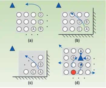
Figure 1a shows a hazardous region that isn’t closed (that is, an exit path exists around the region). In this scenario, sensors A, B, and C can temporarily become a local minimum. Suppose sensor D has already found an escape path. Sensors A, B, and C will eventually find their escape paths via D.
In Figure 1b, sensors A, B, and C are surrounded by a hazardous region. In this scenario, the three sensors should raise their altitudes to a level higher than the alti-tude of at least one sensor in the hazardous region. Assume sensor D has the smallest altitude in the haz-ardous region. With a proper δ, our algorithm will likely guide users to an exit via D.
Figure 1c is similar to the case in Figure 1b except that sensors A, B, and C are all inside the hazardous region, and thus have similar escape paths. In Figure 1d, an exit sensor is in the hazardous region. Sensors A, B, C, and D, which are the exit sensor’s direct neighbors, will guide users to that exit. Sensors that aren’t the exit sensor’s direct neighbors will guide users out of the hazardous region via the shortest paths first, and then to other exits outside of the hazardous region unless no such exits exist. Figure 2 shows how altitude changes occur in a 7 × 7 grid network with D = 2. Three emergency events occur in coordinates (S2, 4), (S6, 7), and (S5, 2), in that order. An exit is located in (S1, 7). Both the side and top views show altitude changes, in decibels (dB). Navigation paths are from sensors with higher altitudes to sensors with lower altitudes.
SIMULATION RESULTS
We first consider a 10 × 10-grid network. Each sensor has four navigation links to neighboring sensors on the east, west, north, and south. We set Aemgto 200 and δ to 0.1.
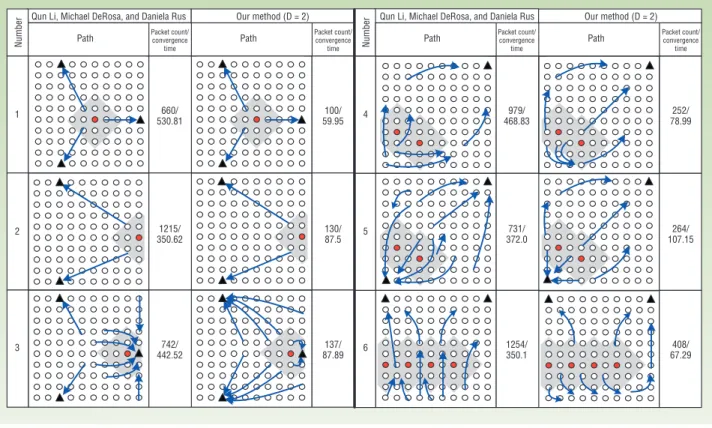
We compare our algorithm with the algorithm pre-sented by Qun Li, Michael DeRosa, and Daniela Rus, using packet count and convergence time as perfor-mance metrics. As the “Related Work in Emergency Navigation” sidebar describes, the packet count doesn’t include packets used during the initialization phase.
We simulate an unslotted Carrier Sense Multiple Access/Collision Avoidance (CSMA/CA) protocol fol-lowing the IEEE 802.15.4 standard3with a data rate of
20 Kbps. We measure convergence time in microseconds (µs).
Figure 3 shows the simulation results. In case 1, the sensor located in the middle of the network detects an A A A A B B B B C C C C D D D (a) (b) (c) (d)
Figure 1. Navigation examples. (a) If an exit path around a haz-ardous region exists, sensors guide the user toward the exit sensor. (b) When sensors are surrounded by a hazardous region, they raise their altitudes to a level higher than the alti-tude of at least one sensor in the hazardous region. (c) Sensors that are inside a hazardous region follow similar escape paths. (d) If an exit sensor is in the hazardous region, the algorithm guides users also in the hazardous region to that sensor.
S1 S2 S3 S4 S5 S6S7 1 3 5 7 S1 S2 S3 S4 S5 S6 S7 1 3 5 7 S1 S2 S3 S4 S5 S6 S7 1 3 5 7 7 6 5 4 3 2 1 S7 S6 S5 S4 S3 S2 S1 7 6 5 4 3 2 1 S7 S6 S5 S4 S3 S2 S1 7 6 5 4 3 2 1 S7 S6 S5 S4 S3 S2 S1 0-1 2-3 4-5 6-7 8-9 10-11 12-13 14-15 16-17 18-19 20-21 22-23 1-2 3-4 5-6 7-8 9-10 11-12 13-14 15-16 17-18 19-20 21-22 23-24 (a) (b) (c)
Figure 2. Examples of altitude changes when emergency events occur in (a) coordinates (S2, 4), (b) coordinates (S6, 7), and (c) coor-dinates (S5, 2). Number Number 1 2 3 4 5 6 660/ 530.81 1215/ 350.62 742/ 442.52 Packet count/ convergence time Path 100/ 59.95 130/ 87.5 137/ 87.89 Packet count/ convergence time Path 979/ 468.83 731/ 372.0 1254/ 350.1 Packet count/ convergence time Path 252/ 78.99 264/ 107.15 408/ 67.29 Packet count/ convergence time Path
Qun Li, Michael DeRosa, and Daniela Rus Our method (D = 2) Qun Li, Michael DeRosa, and Daniela Rus Our method (D = 2)
emergency event. However, the emergency event doesn’t change neighboring sensors’ rel-ative altitudes.
Our algorithm sends few messages and quickly converges.
In case 2, sensor placement is the same as in case 1, except that exit sensor A detects an emergency. Although both algorithms will compute the same navigation paths, Li, DeRosa, and Rus’s algorithm incurs more mes-sages, because sensors near A will first be attracted to, and then repelled from, A.
In case 3, a sensor detects an emergency event near exit A. Without the hazardous regions concept, the system will guide some users through the hazardous region. Because this is undesirable, our algorithm effectively avoids guiding users through the hazardous region.
In case 4, some sensors are bounded by haz-ardous regions. Although guiding users through hazardous regions is inevitable, our scheme will choose paths that are as far away from emergency locations as possible.
In case 5, we add an exit in the lower left corner. Li, DeRosa, and Rus’s algorithm directs some sensors to pass through the haz-ardous regions to reach that exit, but our algo-rithm avoids this problem.
In the scenario in case 6, emergencies almost partition the network. Again, our algorithm discovers safer navigation paths than Li, DeRosa, and Rus’s algorithm.
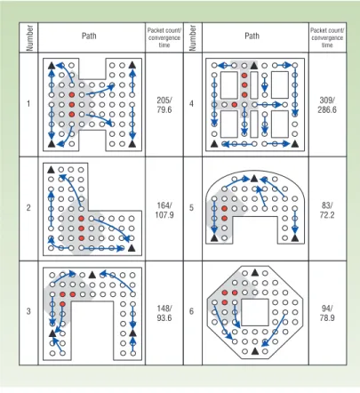
Figure 4 illustrates our navigation results in various network configurations. The results show that our scheme effectively leads people to exits and helps them avoid hazardous regions. They also imply that our protocol is applicable to various building types.
We’ve also simulated our algorithm in a large-scale sensor network with 2,500 sensor nodes. The algorithm selects between 1 and 5 percent of random sensors as exits, and it selects 1 percent of random sensors as emer-gency points. We set the parameter D to 5. The convergence times of 1 to 5 percent of the exit sensors are 21.6 seconds, 10 seconds, 9.1 sec-onds, 2.9 secsec-onds, and 2.0 secsec-onds, respec-tively. These results demonstrate our algo-rithm’s scalability in large networks.
In addition to reflecting the dangerous range affected by an emergency event, D’s value can also affect the navigation results and system performance.
For a small network, a D that is too large is meaningless because a few emergency events
Number 1 2 3 205/ 79.6 164/ 107.9 148/ 93.6 Packet count/ convergence time Path Number 4 5 6 309/ 286.6 83/ 72.2 94/ 78.9 Packet count/ convergence time Path
Figure 4. Navigation results in various forms of networks.
1 3 5 (a) (b) 204 211 398 Packet count Aemg = 150 Aemg = 300 Network (10 × 10) D Network (10 × 10) 292 274 δ = 0.3 δ = 0.3 Packet count Packet count 256 257 δ = 1.1 δ = 1.1 Packet count Packet count 244 249 δ = 5.0 δ = 2.0 Packet count Packet count
Figure 5. Effect of parameters on system performance. (a) Effect of D on the quality of escaping paths and message overheads. (b) Effects of δ and Aemgon the quality of escape paths and message overheads.
can result in a network that’s entirely covered by haz-ardous regions. Figure 5a shows different settings of D in a 10 × 10 grid network. A small D can result in users being guided along paths close to emergency sources. Although a large D can help users find safer paths, it also increases the message overhead.
Figure 5b shows the effects of Aemgand δ and on escape
path quality and message overhead. Using a small Aemg
with a large δ might make it easier to guide users across hazardous regions, as in the third case in Figure 5b. A larger δ can quickly increase the altitudes of sensors with local minimum to values larger than sensors in haz-ardous regions. We thus recommend using a relatively large Aemgwith a relatively small δ. In our current design,
we configured parameters D, Aemg, and δ at the
deploy-ment stage, and we can use manual simulations to deter-mine them.
PROTOTYPE EXPERIENCES
Our prototype system uses MICAz Mote radio plat-forms (www.xbow.com/Products/productsdetails.aspx? sid=3) and incorporates photo sensors, which read light degrees, to simulate and trigger emergency events. In the system, a light degree above a threshold indicates an emergency event, and a sensor reading this light degree will broadcast EMG packets. Because broadcast
com-munications are unreliable,4packets can be lost. Sensors
therefore periodically rebroadcast EMG packets to improve reliability.
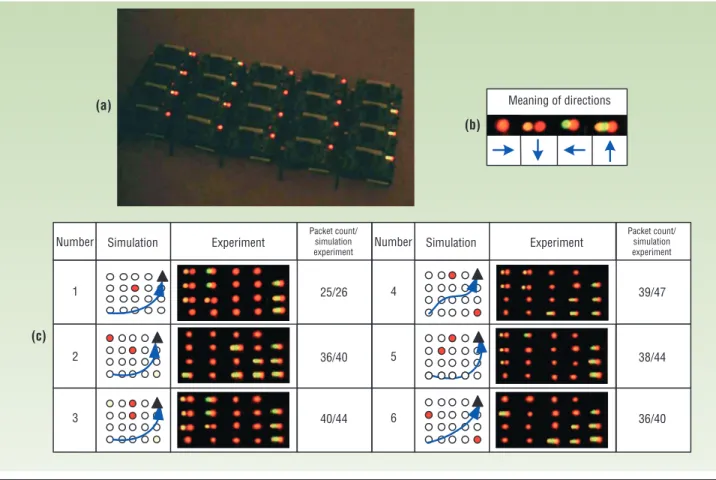
Figure 6a shows the testing of a 4 × 5 grid network. The motes’ light-emitting diodes (LEDs) indicate navi-gation directions, as Figure 6b shows.
Figure 6c shows results from our simulation and experimental testing of the network, including message costs and navigation paths. Because of packet loss, the experimental results show a slightly higher message overhead. Because the network is small, the navigation paths in both the simulations and the experiments are exactly the same.
A
s part of our future research, we plan to im-prove the user interfaces, such as the LED dis-play. We will also extend the results to 3D environments. ■Acknowledgments
The following organizations cosponsor Yu-Chee Tseng’s research: the National Science Council under grant num-ber 93-2752-E-007-001-PAE; the Institute for Information Industry under the Communications Software Technology Figure 6. Simulation and experimental results. (a) A mote’s light-emitting diodes during an experiment; (b) LEDs indicate naviga-tion direcnaviga-tions; (c) comparison of results.
Meaning of directions Number Packet count/ simulation experiment Experiment Simulation 1 25/26 2 36/40 3 40/44 Number Packet count/ simulation experiment Experiment Simulation 4 39/47 5 38/44 6 36/40 (a) (b) (c)
Project; the Ministry of Economic Affairs ROC under grant number 94-EC-17-A-04-S1-044; the Industrial Technology Research Institute, Taiwan; and Intel.
References
1. C-Y. Lin and Y-C. Tseng, “Structures for In-Network Mov-ing Object TrackMov-ing in Wireless Sensor Networks,” Proc.
Broadband Wireless Networking Symp. (BroadNet), IEEE CS
Press, 2004, pp. 718-727.
2. V.D. Park and M.S. Corson, “A Highly Adaptive Distributed Routing Algorithm for Mobile Wireless Networks,” Proc.
IEEE INFOCOM, IEEE Press, 1997, pp. 1405-1413.
3. IEEE Std. 802.15.4, IEEE Standard for Information
Tech-nology—Telecommunications and Information Exchange Between Systems—Local and Metropolitan Area Networks Specific Requirements Part 15.4: Wireless Medium Access Control (MAC) and Physical Layer (PHY) Specifications for Low-rate Wireless Personal Area Networks (LRWPANs),
IEEE, 2003.
4. Y. C. Tseng, S-Y. Ni, and E- Y. Shih, “Adaptive Approaches to Relieving Broadcast Storms in a Wireless Multihop Mobile Ad Hoc Network,” IEEE Trans. Computers, vol. 52, no. 5, 2003, pp. 545-557.
Yu-Chee Tseng is the chair and a professor in the
Depart-ment of Computer Science at National Chiao Tung Uni-versity. His research interests include mobile computing, wireless communication, and parallel and distributed com-puting. He received a PhD in computer and information science from Ohio State University. Tseng is a member of the ACM and a senior member of the IEEE. Contact him at [email protected].
Meng-Shiuan Pan is a PhD student at National Chiao Tung
University. His research interests are wireless sensor net-works and mobile computing. He received an MS in com-munications engineering from National Tsing Hua University. Contact him at [email protected].
Yuen-Yung Tsai is an MS student at National Chiao Tung
University. His research interests are wireless sensor net-works and mobile computing. He received a BS in computer science from National Chiao Tung University. Contact him at [email protected].
![[102-2] WNFA lab4 - A Tiny Wireless Sensor Network](data:image/gif;base64,R0lGODlhAQABAIAAAP///wAAACH5BAEAAAAALAAAAAABAAEAAAICRAEAOw==)