SPECIAL SUBGRAPHS OF WEIGHTED VISIBILITY GRAPHS

(1)

Information Processing Letters 43 (1992) 69-75 North-Holland

24 August 1992

Special subgraphs of weighted

visibility graphs *

F.R. Hsu **

Institute of Computer Science and Information Engineering, National Chiao Tung University, Hsinchu 30050, Taiwan, ROC

R.C.T. Lee

National T~Gng Hua University, Hsinchu 30043, Taiwan, ROC

R.C. Chang

Institute of Information Science, Academia Sinica, Taipei, Taiwan, ROC and Institute of Computer and Information Science, National Chiao Tung University, Hsinchu 30050, Taiwan, ROC

Communicated by M.J. Atallah Received 21 August 1991 Revised 13 April 1992

Keywords: Analysis of algorithms, computational geometry

1. Introduction

A visibility graph G = (V, E) of a polygon P is

defined as follows: Nodes in V are adjacent if and only if the associated vertices in P are mutually visible and the weight of an edge in E is equal to the Euclidian distance between the associated vertices in P. For example, the visibility graph of the polygon in Fig. l(a) is shown in Fig. l(b). A

weighted visibility graph of a polygon is a visibility graph of this polygon and the weight of an edge of this graph is the Euclidian distance between the associated vertices in this polygon.

Correspondence to: Professor R.C.T. Lee, National Tsing Hua University, Hsinchu 30043, Taiwan, ROC. Email: rctlee@nthu.edu.tw.

* This work was partially supported by a grant from the National Science Council of the Republic of China under grant no. NSC80-0408.E009-07.

* * Email: frhsu@twnctuOl.bitnet.

In this paper, we are interested in finding a subgraph of a weighted visibility graph G with a small number of edges such that any arbitrary shortest path on G is almost entirely covered by the subgraph. For example, in Fig. 2, consider a subgraph of the weighted visibility graph of the polygon in Fig. l(a). The shortest path between a

and

f

is abdgf which is fully covered by this subgraph. The shortest path between a and h is abh. Only bh is not covered by this subgraph. In this paper, we show that for any arbitrary weighted visibility graph G of an n-gon, there exists a subgraph with only a linear number of edges such that for any arbitrary shortest path of G, there are most 8 log*n + 5 edges that do not appear in the subgraph. Note that log*n is defined to be the number of applications of the logarithm function required to reduce n to a constant value (say 2). Given an n-gon, we also propose an O(n) time algorithm to find such a subgraph.

(2)

2. Preliminaries

In this section, we introduce some preliminary definitions and geometric properties.

2.1. The polygon cutting theorem and decomposi-

tion tree

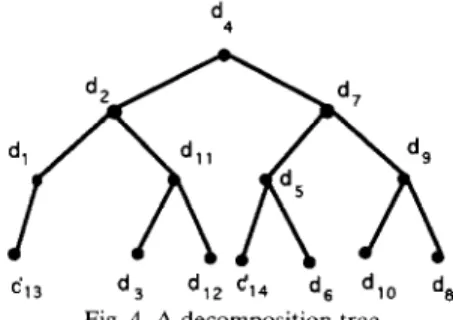
Chazelle [l] proved that for any simple polygon with at least four vertices, there is a diagonal that divides this polygon into two subpolygons, roughly of equal size. More precisely, each of the subpolygons P, and P, generated by this splitting has at least l(n + 5)/31 sides. Consider Fig. 3. The diagonal d, is such a diagonal. If we apply Chazelle’s Theorem recursively, then we obtain a decomposition tree. The decomposition tree for the triangulation shown in Fig. 3 is shown in Fig. 4.

2.2. Hourglasses

Let us introduce an interesting structure, the

hourglass [5]. Suppose that d, has endpoints A and B, d, has endpoints C and D and BACD is a subsequence of the vertex sequence of a polygon P. The union of the shortest path between A and C and the shortest _- path between _- B and D is _-- the hourglass of AB and CD, denoted H(AB, CD). Note that each of the paths is inward convex. There are two types of hourglasses. If the paths are disjoint, we call it open and it is composed of two inward convex chains. If the paths are not disjoint, we call it closed. See Fig. 5 for examples of hourglasses.

An interesting property of hourglasses is that an hourglass can be obtained by concatenating

9 h .

\ f Fig. 2. A subgraph of a weighted visibility graph.

two hourglasses and only two new edges are introduced. There are of course many possible cases which we shall not describe here. Interested readers may consult [51.

2.3. The factor graph

A factor graph is constructed out of a decomposition tree [3,5]. Let us consider the decomposition tree in Fig. 4. Note that the subtree of each node is the decomposition tree corresponding to a subpolygon. For instance, the tree under node

d, corresponds to the entire polygon. For the subtree under node d,, which is shown in Fig. 6(a), the corresponding subpolygon is shown in Fig. 6(b). Let Pd denote the subpolygon corresponding to the ‘subtree under node dj in the decomposition tree. Thus, the subpolygon in Fig. 6(b) will be denoted as Pd,. Now consider Pd,, which is shown in Fig. 7. Diagonal d, has three ancestors, namely d,, d,, and d,, in the decom- position tree. Among them, d, and d, are bound- aries of Pd,. Note that for every subpolygon Pdj, except the boundaries of the original polygon, the boundaries of Pd, must be ancestors of dj in the decomposition tree.

A factor graph is constructed out of a decomposition tree by adding edges from the node

(3)

Volume 43, Number 2 INFORMATION PROCESSING LETTERS 24 August 1992

Fig. 3. A triangulated polygon and its dual tree.

613 d3 d,, 614 2, d,, d, Fig. 4. A decomposition tree

corresponding to dj to all of the nodes corre- sponding to diagonals bounding Pd unless the node is already a parent node of the’ node corresponding to dj. For the subpolygon in Fig. 7, both d,nd d, are boundaries of Pd,. Thus d,d, and

d,d, are in the factor graph. We do not have to

add an edge from d,, to d, because d, is already a parent of d,,. The entire factor graph corre- sponding to the decomposition tree in Fig. 4 is now shown in Fig. 8.

Let us imagine that we want to find the hourglass between d, and d,. From the factor graph shown in Fig. 8, d, is again the lowest common

Fig. 6. A subtree and its corresponding subpolygon.

6

Fig. 7. Subpolygon Pd,

d ₁₃ _d, _d,2 _d14 _d, _dlo _d, Fig. 8. A factor graph.

ancestor of d, and d,. The path between d, and

d, is d, -d, + d,. We can construct H(d,, d4) by constructing H(d,, d,) and H(d,, dJ and then concatenating them. Note that on the factor graph, there is a path between d, and d,, which is d, - d, + d,. Thus we need only construct the

(4)

hourglass H(L14, d7) and then H(d,, d,). From the factor graph, we can also see that H(d,,, d,) will involve the following hourglasses: H(d,,, d,,), H(d,,, d,), H(d,, d,) and H(d,, d,).

That the factor graph which is sufficient for our purpose can be found in [5].

3. A necessary condition

In this section, we shall show that for any arbitrary weighted visibility graph of an n-gon, there exists a subgraph with only a linear number of edges such that for any arbitrary shortest path there are most 8 log*n + 5 edges that do not appear in the subgraph. Given an n-gon, we also propose an O(n) time algorithm to find such a subgraph.

Now let us define some new terms. The modified factor graph is defined as follows: Let U denote the set of nodes in the decomposition tree, each of which having at least log4n descendants. The modified factor graph is constructed out of the factor graph by adding edges from each node in U to all its descendants that are also in U if there is no edge in the factor graph linking these nodes. In the rest of this paper, let

F and S denote the factor graph and the decom-

position tree respectively.

Fig. 9. A leap graph.

A leap graph L is a generalization of the modified factor graph. Let U, be the set of nodes with at least log4n descendants in the decomposition tree S. For i = 1, 2,. . . , log*n, let U, be the set of nodes in S whose numbers of descendants are less than (log%)4 and not less than (log”+ ‘)n14. Note that logCk’n = log logCk-‘)n and 1og’“‘n = n. These nodes also exist in the factor graph F. A leap graph is constructed out of a factor graph by adding edges from nodes of U, in

F to all their descendants that are also in Ui, for i=o, 1 , . . . , log*n. If these edges are already in

F, they will not be added into L again. See Fig. 9.

We now prove that the size of L is O(n).

Lemma 1. The number of edges of a leap graph is

O(n).

Proof. Since the decomposition tree S is balanced, there are at most O(n/(log(‘+ 1)n>4> nodes in S with at least 0(00g~it’~n14) descendants. Thus, the cardinality of q. is only O(n/ (log(if’)n)4). F urt ermore, h since S is balanced and the number of descendants of any node in U, is at most (log(‘)n)4, each node in U, is reached by at most 4 log@+ ‘) n additional edges from its ancestor. Therefore, there are at most O(n/

(log”+ ‘)nj3) edges added from nodes in Ui to all

of their descendants in Ui. Thus the total number of edges added to F is

= O(n/(log n)‘) + O(n/(log log n)‘) + O(n/(log log log n)‘) + . . . = O(n).

Since the size of the factor graph is O(n), the number of edges of a leap graph is O(n). 0

Let us define some new terms before dis- cussing the properties of the leap graph. A diagonal sequence D = Cd,,, drz,. . . , d,,) is serially

concatenable if d,+, separates drl and d,+z in

the original polygon for 1 < t <k - 2. It 1s not difficult to see that any subsequence of a serially

(5)

Volume 43, Number 2 INFORMATION PROCESSING LETTERS 24 August 1992 concatenable diagonal sequence is also serially

concatenable. The following lemma points out an important property of the leap graph.

Lemma 2. For every d,, dj in the decomposition

tree S, there exists a serially concatenable diagonal sequence Cd,, = di, d_,. . , , drl = dj) such that t G 4 log*n + 3 and dr,dr,+, in the leap graph L for 1<1<t--I.

Proof. For di and dj E S, let d’ denote the lowest common ancestor of di and d, in S. By the definition of S, d’ separates di and dj in the

I -

original polygon. If did EL and d,d EL, then the lemma is true.

-

Consider that case that either d,d 6 L or

-

d,d’E L. Suppose that did EL. Let Next(d,, d4) denote the lowest diagonal among diagonals that are on the path from d, to d, in S and separate

d, and d, in the original polygon. If d, is the

parent of d,, let Next(d,, d,) = d,. Consider the diagonal sequence DS = Cd,, = di, dkZ,..., dks =

d’) where dk,+, =Next(d,, d’) for l<l<s--1.

By the definition of Next(dr, d,), it is not diffi- cult to see that DS is serially concatenable. We now further show that dk,dk,+, E F for 1 G 1 <s -

1.

Consider dkldkl,,. If dk,+, = d’, by definition, dkldkl+l is in F. Consider the case that d, ₁₊₁f d’. By definition, dkl+, separates dkl and d’. Assume that d kl+,dkl is not in F. By the definition of S,

d k,+, is a boundary of PLSoNCdk 1+1) and

P RsoMd,,,,) Since dk,+, is an ancestor of d,, in

‘,

'd, “is a subpolygon of

P f

PLSONCdk

if, 1 Or RSON(dk,, ,)’ 171 Since dk,+,dk, is not in F,

d kl+, is not a boundary of Pd . Therefore, there must be some diagonal, say dy: which separates

d k,+, and d,, and is on the path from d,, to dk,+,

in S. Since dk,+, separates d’ and d,, and dj separates dk,+, and dkl, d,’ must separate d’ and

dkl. Besides, d,’ is younger than dk,+, in S, a contradiction. Thus dkl,,dk, must be in F. There- fore, &,dkl+, ~Fforl~l~s-1.

For 0 <t < log*n, let LD(t) and HD(t) de- note the lowest and highest diagonals in U, that are also in DS. If no such diagonals exist, let these notations denote empty. Consider the sub-

sequence DS’ = (dp = d,,, dfZ,. . . , d, = d’) of

DS, where DS’ is composed of LD(t) and LID(t)

for 0 G t G log*n. Consider d,d,+,. If d,+, is also the successor of d, in DS, then d,d, _,ClE F.

If %+I is not the successor of d, in DS, d, and

df,+, must be in the same U,. Therefore,

d,d,+, E L. Since DS is serially concatenable, DS’ is also serially concatenable. To sum up, for

-

the case that d,d P L, there exists a serially con- catenable diagonal sequence DS’ = (df, = di,

drz, . . . > d, = d’) such that e G 2log*n + 2 anddfidf,_l’ELforl<lge’-l.Ifdjd’@L,we

similarly can show that there exists a serially concatenable diagonal sequence DS; = Cd,; =

d’, d,;, . . . , dfi, = dj) such that e’ G 2 log*n + 2

and df,df,+ I EL for 1 < I< t - 1. Since d’ sepa-

rates di and d,, it follows that the combination of

DS’ and DS; is serially concatenable. Therefore, there exists a serially concatenable diagonal sequence (d,, = di, dr2,. . . ,d,, =d,) such that t < 4 log*n + 3 and dr,dr,+, E L for 1 G 16 t - 1. 0 Now we can show a necessary condition of the weighted visibility graph in the following theorem.

Theorem 3. For any arbitrary weighted visibility

graph of an n-gon, there exists a subgraph with only a linear number of edges such that for any arbitrary shortest path, there are most 8 log ‘n + 5 edges that do not appear in the subgraph. There exists an algorithm to construct such a subgraph in

O(n) time.

Proof. Recall that by definition, an hourglass consists of two shortest paths. Let SL denote the shortest path set defined by the hourglasses corresponding to edges in the leap graph L. Let

US(SL) denote the union of SL. We will show

that US(SL) satisfies the statement in the theorem.

For any arbitrary vertices p and q of P, let

~(p, q> denote the shortest path between p and q inside P. Let d, be a diagonal incident to p if

one exists, or otherwise the diagonal closest to p that separates p from q. We define d, in the similar way. By lemma 2, there exists a serially

(6)

concatenable diagonal sequence DS = (d,, =

d,, dr2,. . . , d,,=d,) such that t<4log*n+3

and dr,dr,+, EL for l<l<t-1. Since DS is serially concatenable, H(d,, dq> can be con- structed by concatenating H(d,,, dr2), H(d_,

d,.J.. . ,fU,,_,, d,,). It follows that H(d,, d,)

can be constructed by concatenating at most 4 log*n + 2 hourglasses corresponding to edges in L. Concatenating two hourglasses introduces only two new edges. Thus, it introduces at most 8 1og”n + 2 new edges to construct H(d,, dq> from USCSL). Since at most three line segments of ~(p, 4) are not covered by H(d,, d,), it fol- lows that there are at most 8 1og”n + 5 edges of ~(p, s> not covered by US(SL).

Consider the problem of constructing US(SL). Since US(SL) is the union of shortest paths asso- ciated with hourglasses corresponding to edges in

L and whenever an hourglass is found, its two associated shortest paths are also found, we can construct US(SL) \by constructing hourglasses corresponding to edges in L. Consider the hour- glasses corresponding to edges in L. Let f(k) be the time complexity of triangulating a k-gon. Guibas and Hershberger [51 proposed an f(zz> time algorithm to construct hourglasses corresponding to edges in F and these hourglasses can be stored in O(n) space such that for di and its descendant dj, H(d,, dj) can be constructed in 0(log2 I Pd I) time. Since currently, the best bound for f(k) ib O(k) [2], Guibas and Hershberger’s algorithm [5] can be run in linear time. Consider hourglasses corresponding to edges in L \F. By definition, for any d, in Ui, 1 Pd, I is at most 0((log%>4>. Thus, for d,,d, in ZJ, and d,d, in L,

we can construct H(d,, d,) in

0(log2(log(‘)n)4) = 0((log”+“n)2)

time. As shown in the proof of Lemma 1, there are at most 0(n/(log(i+‘&z)3) edges added from nodes in U, to all of their descendants in Ui. Thus, we can construct hourglasses corresponding to edges added from nodes in U, to all of their descendants in lJ in

o( U(log “+l$z)3)O((log”+‘)n)2) = O(n/log”+%z).

It follows that we can construct hourglasses corresponding to edges in L \ F in

1og*n

i=O

= O( n/log n) + O( n/log log zz) + O( n/log log log zz) -t . . . = O(n).

Therefore, the hourglasses corresponding to edges in L can be constructed in O(n) time and space. It follows that

US(SL)

can be constructed in O(n) time and space. 0

4. Conclusion

In this paper, we are interested in some theo- retical properties of weighted visibility graphs. We show that for any arbitrary weighted visibility graph of an n-gon, there exists a subgraph with only a linear number of edges such that for any arbitrary shortest path, there are most 8 log*n + 5 edges that do not appear in this subgraph. Given an n-gon, we also propose an O(n) time algorithm to find such a subgraph. It is a chal- lenge to design a fast algorithm to find such a subgraph with minimum weight. It should be noted that we are not suggesting that this subgraph should be used as data structure to find shortest paths. The following problem remains open: for any arbitrary weighted visibility graph of an n-gon, does there exist a subgraph with O(n) edges such that the maximum number of missing edges of any arbitrary shortest path is less than O(log * n)?

References

[l] B. Chazelle, A theorem on polygon cutting with applications, in: Proc. 23th Ann. IEEE Symp. on Foundations of Computer Science (1982) 339-349.

[Z] B. Chazelle, Triangulating a simple polygon in linear time, Discrete Cornput. Geom. 6 (1991) 485-524.

[3] B. Chazelle and L. Guibas, Visibility and intersection problem in plane geometry, Discrete Comput. Geom. 4 (1989) 551-581.

(7)

Volume 43, Number 2 INFORMATION PROCESSING LETTERS 24 August 1992 [4] L. Guibas, J. Hershberger, D. Leven, M. Sharir and R.E.

Tarjan, Linear time algorithms for visibility and shortest path problems inside triangulated simple polygons, AIgo- rithmica 2 (1987) 209-233.

[5] L.J. Guibas and J. Hershberger, Optimal shortest path queries in a simple polygon, J. Comput. System Sci. 39 (1989) 126-152.

[6] J. O’Rourke, Art Galley Theorems and Algorithms (Ox- ford University Press, New York, 1987).

[7] M. Overmars and H. van Leeuwen, Maintenance of con- figurations in the plane, J. Comput. System Sci. 23 (1981) 166-204.