國
立
交
通
大
學
應用化學系
碩
士
論
文
利用電荷自洽密度泛函緊束縛方法探討導電高
分子和碳奈米結構的幾何、電性和振動性質
Geometric, electronic, and vibrational
properties of conductive polymers and
carbon nanostructures studied using the
SCC-DFTB method
研 究 生:李文凡
指導教授:魏恆理 教授
利用電荷自洽密度泛函緊束縛方法探討導電高分子和碳奈米結構的幾何、電性和 振動性質
Geometric, electronic, and vibrational properties of conductive polymers and carbon nanostructures studied using the SCC-DFTB method
研 究 生:李文凡 Student:Wun-Fan Li
指導教授:魏恆理 Advisor:Henryk Witek
國 立 交 通 大 學
應 用 化 學 系
碩 士 論 文
A ThesisSubmitted to Department of Applied Chemistry College of Science
National Chiao Tung University in partial Fulfillment of the Requirements
for the Degree of Master
in
Applied Chemistry
June 2009
利用電荷自洽密度泛函緊束縛方法探討導電高
分子和碳奈米結構的幾何、電性和振動性質
學生:李文凡 指導教授:魏恆理
國立交通大學應用化學系
摘要
電荷自洽密度泛函緊束縛方法(以下簡稱 SCC-DFTB)已被成功地應用在不同 的化學系統的結構,電性,和振動性質上:1.共軛雜環高分子, 2.奈米鑽石, 3. 多環芳香族化合物-石墨片和 HPB 分子, 4.單層和多層富勒烯, 5.奈米碳管。 我們觀察了一些新的題目。1.對於共軛雜環高分子的研究,包括順-反式聚乙 炔,聚環戊二烯,聚吡咯,聚呋喃,和聚噻吩。我們探討了能階差,電子態密度, 偶極矩,四極矩和極化率等等的性質。這些性質整體而言呈現了收斂的行為。2. 對於奈米鑽石,我們計算了四面體和八面體結構之奈米鑽石的拉曼光譜。這些光 譜擁有實驗得到之鑽石拉曼光譜特有的位於 1332 波數的訊號。3.多環芳香族 化合物的拉曼光譜已經以電荷自洽密度泛函緊束縛方法計算得到。4.我們已經 計算得到了單層富勒烯的電子和振動性質。我們也探討了內嵌水分子和乙炔之富 勒烯包合物的振動光譜。我們發現如果外層的富勒烯足夠大,則裡面分子的振動 光譜訊號會完全被外層富勒烯遮蔽。5.我們運用了兩種不同的 SCC-DFTB 分散力 模型計算了C @C60 240的位能面.這兩種分散力模型分別是 Slater-Kirkwood 形式 和 Lennard-Jones 形式。在以 Lennard-Jones 模型得到的結果中,C 轉動的能60 障僅僅只有1.62 Kcal/mol。這指明在室溫之下,C 能在60 C240裡面自由轉動,並且位能面上存在許多局部的最小值。對於多層富勒烯之 0 結構的研究結果和 60 240 C @C 的位能面研究一致:對於只有單層差距的多層富勒烯(C @C60 240, 240 540 C @C ,和C @C60 240@C540),內層富勒烯會坐落在中心點。而對於更大層距 的多層富勒烯(C @C60 540,C @C60 960,和C240@C960),內層富勒烯傾向停留在外 層富勒烯壁的附近。多層富勒烯之振動光譜的結果和富勒烯包合物的結果相似。 這些光譜指出,只要外層富勒烯的尺寸足夠大,內層富勒烯的訊號就會被遮蔽。 5.我們計算了不同尺寸和長度之扶手椅型單層奈米碳管的的拉曼光譜。即使是 在此研究中最長的碳管模型:15 奈米的(5,5)單層奈米碳管,朝著實驗所得之 單層奈米碳管拉曼光譜的收斂仍未達到。目前的研究闡述了 SCC-DFTB 方法對於 研究大分子性質和這些性質收斂至固態材料的能力和限制。
Geometric, electronic, and vibrational
properties of the conductive polymers and
carbon nanostructures studied using the
SCC-DFTB method
Student: Wun-Fan Li Advisor: Henryk Witek
Department of Applied Chemistry
National Chiao Tung University
Abstract
The SCC-DFTB method has been applied for studying the geometrical, electronic, and vibrational properties of various chemical systems. The systems can be divided into following categories: 1.conjugated heterocyclic polymer chains, 2.nanodiamonds, 3.polycyclic aromatic hydrocarbons (PAHs) including graphene flakes and hexa-peri-benzacoronenes (HPBs), 4.single and multi-shell fullerenes and, 5.carbon naotubes. Several new topics have been investigated. 1. The study on the conjugated heterocyclic oligomer chains, including trans-cisoid polyacetylene, polycyclopentadiene, polypyrrole, polyfuran, and polythiophene, shows overall convergent behavior of ramous properties including HOMO-LUMO gaps, DOS, dipole moment, quadrupole moment and polarizability. 2. For nanodiamonds, the Raman spectra of both series of octahedral and tetrahedral diamonds show an evidence of the unique peak at 1332 cm-1, which was previously observed in
experimental Raman spectra of diamond. 3. The Raman spectra of the finite PAHs have been computed out using the SCC-DFTB method. 4. The electronic and vibrational properties of single-shell fullerenes have been calculated. The vibrational spectra of endohedral fullerenes with inserted water and acetylene molecules have been discussed for different size of the encapsulating fullerene. It is found that when the cage is large enough, the signal from the inner molecule is completely shielded by the fullerene cage. The PES of C @C60 240 have been scanned with two types of dispersion-corrected SCC-DFTB models, Slater-Kirkwood type and Lennard-Jones type. The energy barrier for C to rotate is merely 1.62 Kcal/mol in the LJ scheme, 60 which indicates that C can freely rotate at room temperature and there exist many 60 energy local minima in the PES. The geometric structures of multi-shell fullerenes are in accord with the C @C60 240 PES study: for the multi-fullerene cages with only one shell difference (C @C60 240,C240@C540, and C @C60 240@C540), the inner fullerene is located in the center. But for the aggregates with larger spacing between shells (C @C60 540,C @C60 960, and C240@C960), the inner fullerenes prefer to stay near the outer cage. Vibrational spectra of the multi-shell fullerenes lead to similar conclusions as those of the endohedral molecule-fullerene complexes. They show that if the cage is large enough, the signal from the inner fullerene is masked. 5. Raman spectra of armchair single–wall carbon nanotubes (SWNT) with different diameters and lengths are presented. The convergence toward the experimental Raman spectra of “infinitely” long SWNT is still not achieved even for the longest studied presently model, i.e. a 15nm (5,5) armchair SWNT. The present study illustrates the capability and limitations of the SCC-DFTB method for studying the properties of large molecules and their convergence toward the corresponding solid state materials.
Acknowledgments
First of all, I would like to give my honest thanks to my advisor Henryk. He gave me a lot of precious guides in my research, and also offered me an opportunity so that I could stay in Nagoya for two months and enjoy the research there. I would like to thank my lab mates: Chien-Pin, Christopher, Amy, and also the former lab mates Mong-Jhu and Chun-Hao. When I entered this lab, I almost knew nothing about quantum chemistry, linux operating system, mathematics, even English. They helped me in every aspect and let me grow fast. Especially I appreciate the help from Chien-Pin. He taught me how to run SCC-DFTB, how to write a code, and also we had many helpful discussions on my research. I would like to thank people who helped me during my stay in Nagoya University. Prof. Irle gave me several interesting topics on the carbon nanostructures and helped me to dig into these topics. I also had a wonderful time with Nishimura-san, Hara-san, Xiao-Mei and Dr. Ying and Dr. Jiang. They were very kind and friendly. I would like to thank my parents who support me both mentally and economically every time when I meet difficulties. Especially, I appreciate my grandmother, who made much effort all the way with my growth. I also would like to thank my partner Tina, we had many precious experiences during these two years and grow up together. Thank the Lord for giving us these treasurable times. The brothers and sisters in church are definitely my firm support. Thank everyone in the brothers’ home, especially Daniel, who relaxes me invisibly. I also thank the dear working saints, the saints of division 407. They are very cute and make me feel warm. I really enjoy and love the church life in 407, enjoy the love among the brothers and sisters. In the end, I would like to thank the Lord, who gave me every experience here and led me through this stage in my life. Like what said in Psalm 23 : Jehovah is my Shepherd;
I will lack nothing. He makes me lie down in green pastures; He leads me beside waters of rest. He restores my soul; He guides me on the paths of righteousness for His name's sake. Even though I walk through the valley of the shadow of death, I do not fear evil, for You are with me; Your rod and Your staff, They comfort me. You spread a table before me in the presence of my adversaries. You anoint my head with oil; my cup runs over. Sure goodness and lovingkindness will follow me all the days of my life, and I will dwell in the house of Jehovah, for the length of my days.
Contents
List of Figures ………... Ⅲ List of Tables ………... Ⅶ
1. Introduction ... 1
2. Theory ... 5
2.1 The Electronic Properties of Condensed Matter ... 5
2.1.1 Band Structure, Density of States (DOS) and Band Gaps ... 5
2.1.2 Dipole Moment and Quadrupole Moment ... 9
2.1.3 Polarizability ... 12
2.2 The Vibrational Properties of Condensed Matter ... 13
2.2.1 Phonons and Vibrational Density of States (VDOS) ... 13
2.2.2 Principles of Raman and Infrared (IR) Spectra ... 16
2.3 The Self-Consistent Charge Density-Functional Tight-Binding (SCC-DFTB)ll Theory ... 19
2.3.1 The Tight-Binding (TB) Theory ... 19
2.3.2 The Density Functional Theory (DFT) ... 21
2.3.3 The SCC-DFTB Theory ... 22
2.3.4 SCC-DFTB + Dispersion Correction ... 25
2.3.5 The Derivation of Harmonic Vibrational Frequency, Raman Activity lll and IR Intensity in the SCC-DFTB Scheme ... 27
3. Technical Details ... 32
4. Results and Discussion ...33
4.1 Conjugated Heterocyclic Polymer Chains ... 33
4.1.1 Evolution of Equilibrium Structures ... 38
4.1.2 Evolution of HOMO-LUMO Energy Gaps ... 45
4.1.3 Evolution of Electronic DOS Distributions ... 47
4.1.4 Evolution of Charge Distribution ... 49
4.1.5 Evolution of Dipole Moments ... 54
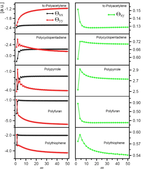
4.1.6 Evolution of Quadrupole Moments ... 57
4.1.7 Evolution of Polarizabilities ... 60
4.2 Raman Spectra of Nanodiamonds ... 67
4.3 Raman Spectra of Polycyclic Aromatic Hydrocarbons (PAHs) ... 78
4.4 Icosahedral Fullerenes ... 83
4.4.1 Geometrical Description of Icosahedral Fullerenes ... 83
4.4.2 Potential Energy Scan (PES) of C60@C240 – Search for the Most lll Stable Structure ... 85
4.4.3.1 Endohedral Fullerenes ... 89
4.4.3.2 Multi-shell Fullerenes ... 92
4.5 Raman Spectra of Single-Wall Carbon Nanotubes (SWNTs) ... 96
5. Conclusions ... 100
List of Figures
Figure 2.1 (a) The schematic band structure of the 1D chain of hydrogen atoms with H-H distance of 1 Å. (b) The corresponding DOS. The shape of the wave function is symbolically represented by circles ………... 6 Figure 2.2 (a) The schematic band structure of the 1D chain of nitrogen atoms with N-N distance of 2 Å. And (b), the DOS of the band structure. The shapes of the wave function are iconized with circles ……... 7 Figure 2.3 The phonon dispersion curves of infinite polyyne chain calculated using the SCC-DFTB method ……….. 14 Figure 2.4 Schematic representation of light scattering processes in matter …. 17 Figure 2.5 Schematic diagram of IR absorption process in matters ………... 18 Figure 4.1 Models of a) the C and b) 2h C symmetric oligomers ... 36 2v
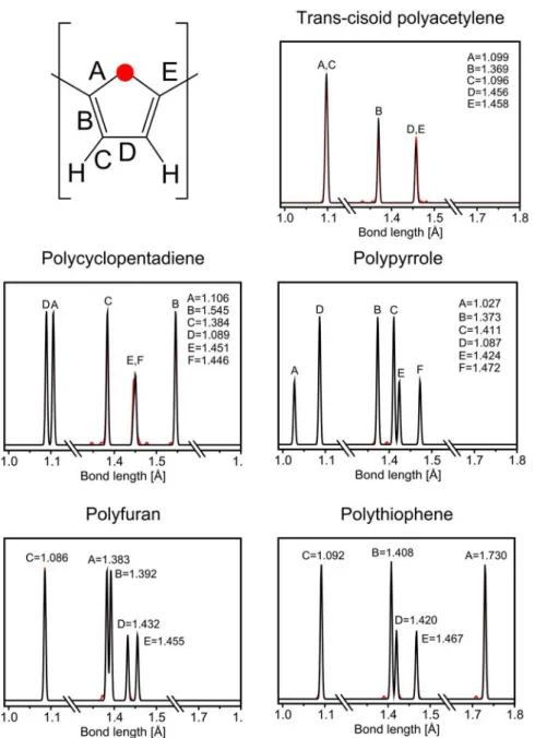
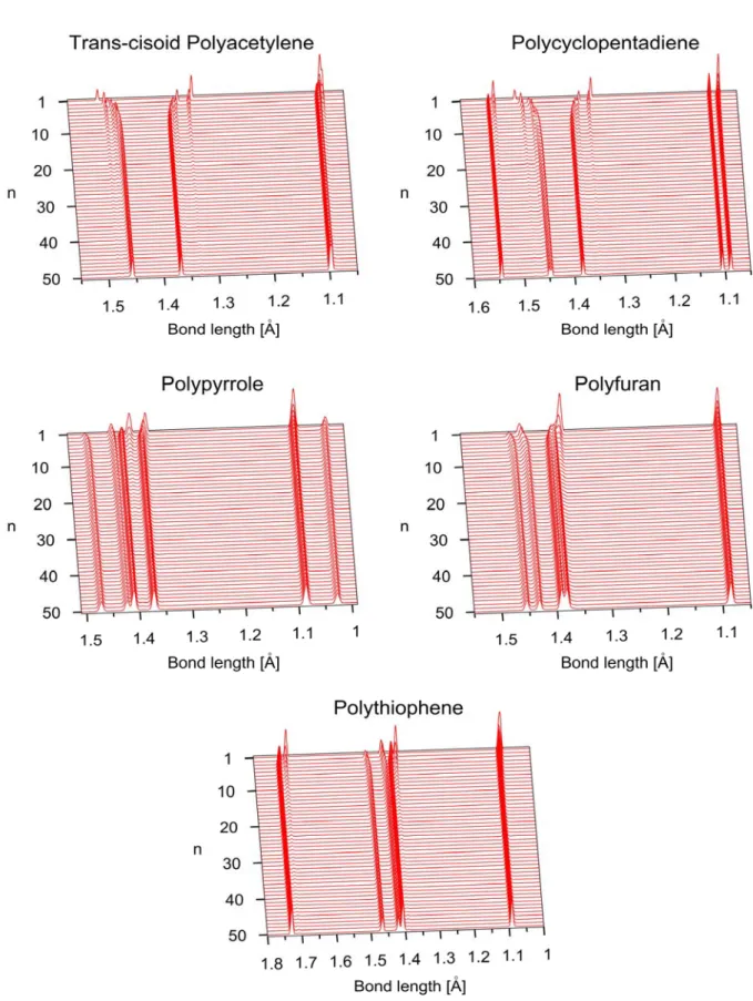
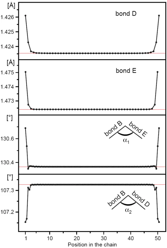
Figure 4.2 Bond length distribution comparisons between the molecular 50-mer (red line) and solid-state polymer (black line) of all the considered models in this study ... 38 Figure 4.3 Bond length distribution convergence of the considered models in this study ... 41 Figure 4.4 Bond length and bond angle distribution of pyrrole 50-mer.
Calculated values of solid state polypyrrole are given in
red solid lines ... 42 Figure 4.5 Band gaps of all the considered models. The values shown are the extrapolated results using second-order polynomial fitting for the last forty points ... 46 Figure 4.6 Electronic DOS distribution convergence of all the considered models. The red areas correspond to the occupied valence bands. The red area and white area are separated by the calculated
Figure 4.7 Induced Mulliken charges of the heteroatoms of the 50-mer in each system. The red solid lines are the corresponding
solid-state values ... 51 Figure 4.8 Induced Mulliken charges along the -conjugated carbon backbone
of the 50-mer in each system. Solid lines in red and blue are
the solid-state values ... 52 Figure 4.9 The evolution of the induced charges on the nitrogen atoms in
oligopyrroles. Value for polymer is given by the solid red line ... 53 Figure 4.10 Evolution of the dipole moments for all the considered models. Only
the dipole moments of molecules with 2m1 unit cells
(C symmetry) are shown ... 57 2v
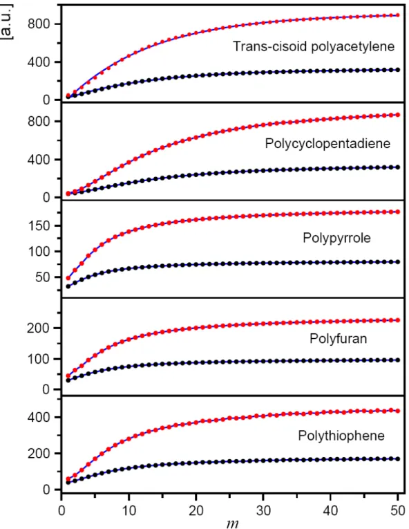
Figure 4.11 Evolution of the quadrupole moment tensor components of all the considered models ... 59 Figure 4.12 Polarizability invariants of all the considered models.
The blue curves are given according to the fitting formulas ... 63 Figure 4.13 The structures, molecular formula, and abbreviations of the
tetrahedral and octahedral nanodiamonds ... 71 Figure 4.14 Comparison of the Raman specra calculated by BLYP/3-31G, SCC-DFTB, and BLYP/6-31G* (A and T2 only)... 72 Figure 4.15 The Raman spectra evolution with respect to the size of the
tetrahedral and octahedral nanodiamonds………....…73 Figure 4.16 The evolution of the T peak in the Raman spectra of the three 2
largest nanodiamonds for tetrahedral and octahedral
nanodiamonds………...74 Figure 4.17 The evolution of Raman spectra for both tetrahedral and octahedral nanodiamonds with “infH” case……….. 75
Figure 4.18 The formation of the band at around 1200 cm-1 of the “infH” tetrahedral nanodiamonds ……….. 76 Figure 4.19 The formation of the band at around 1200 cm-1 of the octahedral
nanodiamonds ………. 77 Figure 4.20 The symmetries and vibration vectors of the D band and G band in
Raman spectra of PAHs ……….. 78 Figure 4.21 Geometries of PAHs. Left: C3 Right: B3...….. 80 Figure 4.22 The deformed B3 obtained by optimization along the imaginary
vibration mode ……….... 80 Figure 4.23 Comparison of the SCC-DFTB and BLYP/3-21G Raman spectra
of C3 and C4 ……….. 81 Figure 4.24 Evolution of Raman spectra of both graphenes and HPBs ……. 82 Figure 4.25 The evolution of Raman spectra of “infH” graphenes
and HPBs ………... 83 Figure 4.26 Structures of the icosahedral fullerenes considered
in this study ……… 85 Figure 4.27 Angles of rotation for C @C60 240 ……….. 86 Figure 4.28 The three different orientations of the benzene dimer ………… 87 Figure 4.29 The potential energy curves of the three different benzene
dimmers ………. 88 Figure 4.30 The PES of C @C60 240using the LJ model. Energy in Hartree .. 89 Figure 4.31 IR spectra of the endohedral fullerenes ……….. 90 Figure 4.32 Raman spectra of the endohedral fullerenes ………... 91 Figure 4.33 Models of all the considered multi-shell fullerenes. Except for
60 240 540
C @C @C , the color of the inner fullerenes are changed to purple for the multi-shell fullerenes ………. 93
Figure 4.34 IR spectra of multi-shell fullerenes ……… 94 Figure 4.35 Raman spectra of multi-shell fullerenes ……… 95 Figure 4.36 Model of (9,9) 5nm SWNT ………... 97 Figure 4.37 Raman spectra of SWNTs considered in this study ………. 98-99
List of Tables
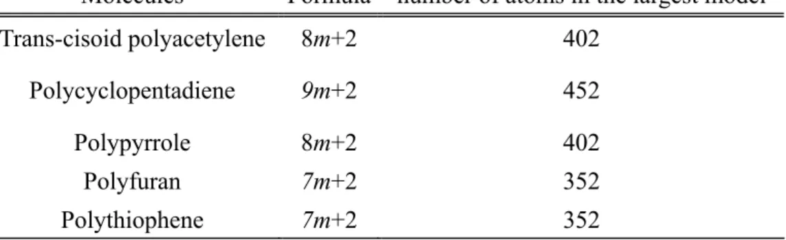
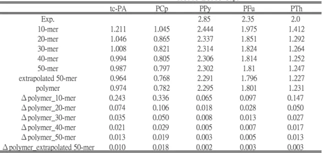
Table 4.1 Molecular formulas for all the considered n = 1~50 molecular models of oligomers….………. 36 Table 4.2 HOMO-LUMO gaps and the differences between the oligomers and the solid-state value……….... 47 Table 4.3 The optimum parameters used eq. 4.3 ………... 64 Table 4.4 Abbreviations, molecular formula, and number of atoms for
Graphenes and HPBs ………... 79 Table 4.5 List of the SWNTs considered in this study ……….. 96
Chapter 1
Introduction
In recent years, owing to the fast development in both the computer hardwares and quantum chemical theories, computational chemistry has become applicable to study larger systems and obtain more accurate results. On the other side, many new important physical observables of solid–state materials like energy band gaps and infrared (IR) and Raman vibrational spectra, can be accessed through experiment. For theoreticians, once the energy of the system at equilibrium is computed, vast of extended properties can be directly gained by differentiating the energy with respect to different variables.1 These include the HOMO-LUMO energy gaps, equilibrium structural information, charge distribution, harmonic vibrational frequencies, etc. If external perturbation is added, the Hamiltonian can be modified to include the perturbation and the properties resulting from the interaction between the molecule and the external perturbation can be calculated. There exist in general two approaches to obtain the above properties for extended systems: molecular approach and the traditional, solid-state approach. The main idea of the molecular approach is using the quantum chemical theories to obtain the properties of interest first at the molecular level. Say, for energy gaps of polymers, one can start the calculation for a monomer and extend gradually the system to longer-and-longer oligomers to obtain the calculated energy gaps as a function of the size of the system. By extrapolating this function one can get the approximate value of the energy gap of the polymer built of infinitely many monomers, which corresponds to the band gap computed within
solid-state approach. The molecular approach ignores the effects that may occur in the real solid-state matters. For example, interactions of building blocks like chain interaction in polymers or layer interaction in graphite, are neglected. Still, the molecular approach has been used extensively and gained constructive results. The second approach, the solid-state method, employs periodic nature in the crystal lattices, this can be done in the reciprocal space introduced by Fourier transformation of the real space quantities.2,3
The Self-Consistent Charge Density-Functional Tight-Binding (SCC-DFTB)4 method had been born and can be applied to material science with the two approaches mentioned above. It is a semi-empirical method based on the second-order Taylor expansion of the density functional theory (DFT) energy with respect to the charge density fluctuation. Although it is a semi-empirical method, it can cope with molecules up to thousands of atoms much faster than the existing ab initio methods without losing much accuracy.5,6 It is a good candidate to perform the calculations for systems containing up to thousands of atoms.
The principal idea of this study is to investigate the following two issues: 1.the evolution of the physical properties with growing molecular size, and 2. the transformation of physical properties from molecular stage toward solid-state stage. We have chosen as the prototypes of the conductive polymer chains, the systems of polypyrrole, polyfuran, polythiophene, trans-cisoid polyacetylene, and polycyclopentadiene. At present, our study of these polymers mainly focuses on the molecular geometrical and electronic convergence toward the infinite polymer. This has been done by examining several properties that will be discussed in Chapter 4. Besides the well-studied conductive polymers, we also have chosen several other carbon-containing materials. First of them is the nanodiamond. For this molecule, we intend to locate the signature of the solid state Raman spectra — the unique 1332
cm-1 peak at the molecular stage. We trace the unique 1332 cm-1 peak. Next, for PAHs, we focus on the evolution of the Raman spectra. The character of the Raman spectra changes with different PAH size7; we are trying to relate the change to their molecular size. The main parameter here is the so-called D/G ratio in the Raman spectra, which is defined as the intensity ratio between the A D (disorder) band and 1g
the E G (graphite) band. The study is still under investigation. The third type of 2g
the carbon-containing systems introduced by us are the well-known fullerene cages. We have been trying to analyze two topics concerning the icosahedral fullerenes. The first issue is signal shielding in the SCC-DFTB Raman spectra of single- and multi-shell fullerenes. The signal shielding effect is discussed for the endohedral and multi-shell fullerenes. The second issue is the scan of the potential energy surface (PES) for C @C , which is meant to give a visualization of a free rotation of 60 240 C 60 inside C240. The last systems being discussed are the single-wall carbon nanotubes (SWNTs). We mainly focus on their Raman spectra. Experimental first-order Raman spectra show only the strong G band for SWNTs.8 For now, we only present brief reprot showing that for the armchair (5,5) SWNTs with length of 15 nm, the Raman spectra displays only the D band, which suggests that the transformation from molecular level toward the solid-state level occurs for larger tubes. Further study will pursue this issue in the future.
In chapter 1, we give a general introduction to the topics studied in this Thesis, which is followed by the extension of various theoretical aspects in chapter 2. Chapter 3 is a brief note on the programs and the parameters we have used for calculation. Chapter 4 gives the results and discussion of the application of the SCC-DFTB method on several systems, including the conductive polymers and the carbon nanostructures. Unfortunately, at this time many of the research are still far from
completion, hence in several paragraphs only concise results are shown. The conclusions of this Thesis are given in chapter 5.
Chapter 2
Theory
2.1 The Electronic Properties of Matter
In the present study, several material properties are investigated. They are generally a subject of interest in solid-state physics. Here, we give concise introduction to each of the properties studied in this Thesis.
2.1.1 Band Structure, Density of States and Band Gaps
In nature, every atom possesses its own set of atomic orbitals, in which the electrons can “reside” in. For example, every hydrogen atom has one 1s orbital, and a carbon atom has one core 1s orbital and four valence orbitals (one 2s orbital and 2px, 2py, 2pz
orbitals). When atoms come together and form a molecule, linear combinations of the atomic orbitals belonging to each atom are made to give the molecular orbitals (MO). This approach is referred to as the linear combination of atomic orbitals (LCAO) method. For the simplest hydrogen molecule, there are two MOs originating from the two 1s AO of the two hydrogen atoms. The number of thus obtained MOs will be equal to the total number of AOs in the molecule.
When the system is expanded from a molecule to a solid crystal, there will be infinitely many orbitals made from the infinitely many AOs. We consider the simplest model: a hypothetical 1D chain built of n equally spaced hydrogen atoms. The unit
(CO), rather than molecular orbitals. The lowest in energy CO will be made by
summing up all the n 1s orbitals with plus signs:
0 1 1 2 3 4 1 1 ... n ( )i j n n j j j j e
, (2.1) which can be interpreted as bonding orbital with zero nodes. The highest in energy CO will be 1 2 3 4 1 1 ... n ( i j) n ( 1)j n n j j j j e
, (2.2) which can be interpreted as an antibonding orbital with n-1 nodes. The mth CO will be( 1) ( 1) 1 2 3 4 ( 1) ( 1) 1 2 3 4 1 ( ... ) ( ) m n m i i n j n n m n j j e e e e e e e
(2.3) The exponential term( 1) ( 1) m j i n e
is called the phase factor, and the coefficient of i, ( 1)
( 1)
m j
n
, is the so-called k vector in the reciprocal space. The k vector is characterized by periodicity, which ranges from 0 to π in this case.
The mathematics behind this formalism is the Fourier transform. A periodic function f(x) which satisfies the condition: f(x) = f(x+a), where a is the periodicity of
function f, can be expanded into a Fourier series. By using Euler’s formula
cos( ) sin( ) inx e nx i nx , we obtain ( ) n inx n n f x c e
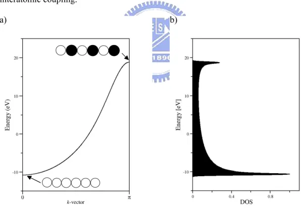
, where cn is the Fourier coefficient.Because the crystal lattice has the periodicity of the lattice translation vectors, the electron motion is also periodic in the lattice, hence can be expanded in a Fourier series. If we now plot the energies of different sets of CO corresponding to different values of k, we obtain the diagram called “band structure”. The band structure of the 1D hydrogen atom chain is shown in figure 19. Because the unit cell contains only one hydrogen atom, and thus only one 1s orbital per unit cell, the only curve in the band structure corresponds to this orbital. In practice, the systems under studied are usually 3D and contains more than on atom in the unit cell. Hence the band structure looks much more complicated. To extract the relevant informationfrom such complicated 3D band structures, people found out a way of doing this by means of the density of states (DOS). The DOS is defined as the number of one electron levels in a small energy interval, or mathematically in the 1D case:
( ) ~ dk D E dE (2.4)
The DOS is a function of band energy E, and it is the inverse slope of the band being considered. That is, the flatter the band, the steeper the corresponding DOS. A very sharp DOS results from an extremely flat, atomic-like band, one that arises from an atomic orbital that does not overlap significantly with neighboring orbitals. Electrons occupied in such a band can not easily move through the crystal and they are slow. On the other hand, a wide DOS indicates rapidly moving electrons due to strong interatomic coupling.
a) b)
Figure 2.1 (a) The schematic band structure of the 1D chain of hydrogen atoms with H-H distance of 1 Å. (b) The corresponding DOS. The shape of the wave function is symbolically represented by circles.
π* π σ* σ σ σ*
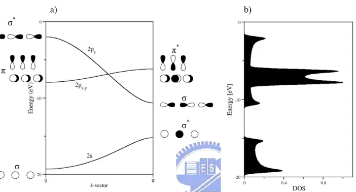
we will have four AOs per nitrogen atom in one unit cell. The resulting band structure, as we can see, contains four valence bands. Note that the 2px and 2py bands are
degenerate in the plot. Note that the partial DOSs come from the three 2p orbitals superpose together in the DOS diagram.
a) b)
Figure 2.2 (a) The schematic band structure of the 1D chain of nitrogen atoms with N-N distance of 2 Å. And (b), the DOS of the band structure. The shapes of the wave function are iconized with circles.
The electrons fill the bands in the same way as they fill the molecular orbitals. The bands are filled according to their energy order, for example, for the 1D atomic chain of nitrogen, the 2s band will be filled by the 2s electrons from each nitrogen atom, and the 2p electrons occupy the 2p bands. The bands filled with electrons are called
valence bands, and the empty bands are called conduction bands. Note that the
valence bands may be only partially filled. Electrons may be excited from the valence band to the conduction band through thermal energy or an external electric field, which results in electric current. The Fermi-Dirac distribution ( )f E gives the
1
( ) 1 exp F / f E E E kT (2.5)In the formula, k is the Boltzmann constant, and T is the temperature Kelvins. The
Fermi level EF is defined as the energy of the topmost filled orbital at absolute zero (T=0). The difference in energy between the top of the highest valence band and the bottom of the lowest conduction band is the so-called band gap. The band gap for solids is corresponding to HOMO-LUMO energy gap for molecules. It is an index of the electrical conductivity of materials and can be used to classify the insulators, semi-conductors, and conductors. In a qualitative perspective, the insulators can be thought as solids with large band gap between the completely filled valence band and the conduction band, and these two bands do not cross at any k point. The semi-conductors are insulators with relatively small band gap (say less than 3 eV)10, thus the electrons can be excited to conduction band by thermal energy. Metals have the highest valence band partially filled, thus no energy gap exists.
2.1.2 Dipole Moment and Quadrupole Moment
The dipole and quadrupole moments describe the properties of the charge distributions inside a molecule. In the classical point of view, atoms or molecules can be regarded as an assembly of point charges with definite positions in space. In quantum mechanical picutre, the definite description of the positions of charges are replaced by the probability distributions in space. Summations over discrete charges are also substituted by integrals over charge distribution probability corresponding to the square of the wave function.
Here we start at the classical level, to see that the molecular charge distribution can be decomposed into a hierarchy of electric moments (monopole, dipole, quadrupole, etc.).11 Consider a collection of discrete charges
i
distances
ri from an arbitrary origin. The resulting potential at some point R is given by 0 1 ( ) 4 i i i q V R R r
, (2.6)where 0is the vacuum permittivity and 0 1
4 is the Coulomb’s constant. For the
condition R >> ri, 1
i R r
can be expanded using the Taylor expansion:
1 1 1 1 1 : ... 2 i i i i r r r R R R R r (2.7)
Here the single and double dots represent tensor contractions. The potential V is then
0 1 1 1 4 ( ) : ... 2 q V R R R R (2.8) The above equation introduces a hierarchy of multipole moments: the charge q (monopole), dipole moment , quadrupole moment, etc. There are still higher order terms, like octupole, hexadecapole, etc., moments. The first three multipole moments are defined as:
( ) ( ) ( ) i i i i i i i i i q q r d r q r r r d r q r r rr r d r
, (2.9)with ( ) r being the charge density.
Note that the charge is a scalar, the dipole moment is a vector, and the quadrupole moment is a tensor. The definitions express the multipole moments either as summations of discrete charges or integrals over continuous charge density. Usually the dipole moment has the unit of Debye. 1D =3.336 10 30 C m .The quadrupole moment is a symmetric square matrix with totally nine components. But only six of
them are independent due to symmetry relations. That is, , where i and j can ij ji be x,y or z. Usually the quadrupole tensor is chosen to be traceless, which means that the sum of the diagonal terms is zero. The traceless is defined as
2 1 (3 ) 2 i i i i i q r r r
I , (2.10)where I is the unit matrix, with diagonal elements equal to one.
The multipole moments introduced above can be used to describe the interaction of electromagnetic field with matter. For example, the energy of a collection of charges subjected to an external field is given by
1
: ... 3
W qV E E (2.11)
Here we use W to denote energy, to avoid the confusion with the electric field E. The picture here is that the total charge q interacts with the potential, the dipole moment interacts with the field, and the quadrupole moment interacts with the field gradient. They contribute additional energy to the total energy in the presence of the electric field.
In the SCC-DFTB framework (which will be introduced later), the Mulliken charge is used to describe the charge q. The electron density ( ) r at certain position r
within a molecule is defined as the square of the MO.1 2 ( )r ( )r
(2.12)
The ith MO in a molecule can be expanded in the LCAO form as described in the previous section,
i ci
(2.13), whereciis the coefficient for the AO . The square of the MO is then 2
i c ci i
We introduce the occupation number (number of electrons), n, for each MO. Then the
total number of electrons N in a molecule can be given by
2 MO AO MO AO MO AO i i i i i i i i i i i N n d n c c n c c S D S
r
(2.15), where S is defined as the overlap matrix of AOs and D is the density matrix given by summing up the multiplications the occupation numbers and the AO coefficients. In computational chemistry, the Mulliken population analysis based on the DS matrix is used for distributing the electrons into the atomic contributions.
The contributions from all AOs located on a given atom A may be summed up to give the number of electrons associated with atom A. In the Mulliken sheme, the contribution involving basis functions on different atoms is divided equally between the two atoms. The Mulliken electron population is thereby defined as
AO AO A A D S
(2.16)The gross charge on atom A is the sum of the nuclear and electronic contributions.
A A A
q Z (2.17)
Here ZA is the number of positive charge that the nucleus owns.
2.1.3 Polarizability
In the presence of the external electric field, the molecular charge distribution may be distorted and leads to modified multiple moments.11 Using the Taylor expansion, the previously discussed electric dipole moment μ can be expanded in a power series in the applied field:
0 E :EE ...
, (2.18)
where 0 is the permanent dipole moment, i.e., the dipole moment in the absence of the external field. is the linear response of the dipole moment to the applied field, called polarizability. Andβis the hyperpolarizability, which describes the leading contribution to the nonlinear response of the dipole in the applied field. The
polarizability is in fact a tensor with nine components: xx xy xz yx yy yz zx zy zz . (2.19)
The polarizabilitry tensor is symmetric, hence only six tensor components are needed to specify the whole tensor. Physically, it is a measure of the easiness that the larger magnitude of the dipole moment can be induced by an external field, or in other words, it is the ratio of the induced dipole and the external electric field.
The total energy of the system can also be expanded using the power series of the electric field. 0 0 1 2 W W E E E (2.20) The polarizability tensor components can thus be expressed in terms of the total energy: 2 0 ij i j E W E E (2.21)
In the case of our SCC-DFTB calculations, the derivative in the equation above is computed numerically.
2.2 The Vibrational Properties of Matter
2.2.1 Phonon Dispersion Relations and Vibrational Density of States
(VDOS)
In crystals, the energy of a lattice vibration is quantized. The quantum of energy is called phonon, similar to photon for light. The relationship of phonon and lattice vibration is in analogy with photon and light.
the number of unit cells should be infinitely many). The total number of vibrational modes for a single unit cell is3 2 6 , because every atom in the unit cell has 3 degrees of freedom. The resulting phonon structure will contain six bands. In accord with the band structure plot, in the phonon dispersion plot, the vertical axis gives the vibrational frequency of the vibrational modes, and the horizontal axis correspond to the k-points used in the Fourier transform. For instance, at k=0, the crystal vibration of the first phonon band (lowest in energy)D1,k0 is formed by summation of the vibrational modes in each unit cell lowest in energy with plus signs over all the M lattices. (0 ) 1, 0 11 12 13 1 1 1 1 ... M i l M (1)l k l l l l D Q Q Q e Q Q
(2.22)The Q denotes the vibrational normal mode lowest in energy of the lth unit cell. 1l
The crystal vibration of the second phonon band at k=0 is given by (0 ) 2, 0 21 22 23 2 2 1 1 ... M i l M (1)l k l l l l D Q Q Q e Q Q
(2.23)Here Q corresponds to the second lowest in energy vibrational normal mode of the 2l lth unit cell. The rest four bands have the same formalism. If atk , the vibraional mode of the whole crystal is given by
( ) 1, 11 12 13 1 1 1 1 ... M i l M ( 1)l k l l l l D Q Q Q e Q Q
(2.24)In general, the crystal vibration mode of the thj phonon band at an arbitrary k point is
composed of the linear combination of the unit cell normal modes as 1 ( ) 1 , 1 1 l M i M ik M j k jl jl l l D e Q e Q
, (2.25)given k the phase factor and also it is the wave vector in solid state physics, which is
defined as
2
k
, (2.26)
with the wavelength of the incident radiation.
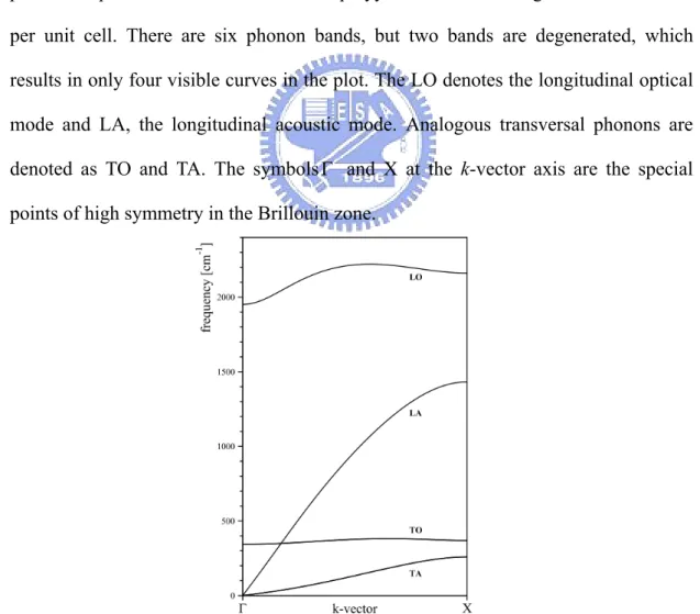
Figure 2.3 The phonon dispersion curves of infinite polyyne chain calculated using the SCC-DFTB method.
the vibration spatial characteristics. These two types of phonons can be divided further into the so called optical or acoustic modes. The optical phonon branches are
named “optical” because in the ionic crystals, these types of modes are easily excited by radiation, and in the vibration the positive and negative ions at adjacent lattice sites swing against each other, creating a time-varying electrical dipole moment. The atoms in the acoustic mode vibrate in the way similar to acoustic waves, that all the atoms or (ions) vibrate in phase. The acoustic modes have zero frequency at k=0, because they
are in fact the translations when all the unit cells move in the same direction.
An example of the phonon dispersion curve is shown in Figure 2.3. This is the phonon dispersion curves of the infinite polyyne chain containing two carbon atoms per unit cell. There are six phonon bands, but two bands are degenerated, which results in only four visible curves in the plot. The LO denotes the longitudinal optical mode and LA, the longitudinal acoustic mode. Analogous transversal phonons are denoted as TO and TA. The symbols and X at the k-vector axis are the special points of high symmetry in the Brillouin zone.
The VDOS is defined analogously like the DOS in band structure theory. The VDOS is given by ( ) k d , (2.27)
with the vibrational frequency.
In the SCC-DFTB VDOS calculation, we take the molecular harmonic vibrational frequencies, smear them along the k-axis with a Gaussian function, and then superpose these Gaussian functions to make the usual VDOS.
2.2.2 Principles of Raman and Infrared (IR) Spectra
Under the radiation of the infrared light, molecules may be excited into their vibrational excited states. There are several phenomena can be observed during the radiation. Among them, the light absorption and emission is responsible for the IR spectrum, and light scattering for the Raman spectrum. A simple description of these two processes is given below.
Light Scattering
In the light scattering, the incident light, or photon, is not absorbed by molecules, but instead, the scattering occurs. As shown in the diagram below, there are three types of scattering. They are Rayleigh scattering, Stokes shift, and anti-stokes shift. Only Rayleigh scattering is elastic, i.e., the photon keeps its initial energyh0after being scattered by the molecule. In the second case, the incident photon losses certain amount of energy, which corresponds to one quantum of vibrational energy equal to vibrational level differencehv of the molecule. Hence the emitted radiation will give a v
signal at the lower energy side with respect to the Rayleigh line in the Raman spectrum. This is the Stokes shift. In the third case, a photon gains more energy after scattering, hence the signal appears at the higher-energy side relative to the Rayleigh
Ground state 1st vibrational excited state
Stokes shift
Rayleigh scattering Anti-Stokes shift Virtual state v v E h 0 i E h Ef h0 Ei h0 0 ( ) f v E h v v E h Ev hv 0 ( ) i v E h Ef h0 line and is called anti-Stokes shift. The later two cases are inelastic processes and are called Raman scattering.
Figure 2.4 Schematic representation of light scattering processes in matter.
Noteworthily, these processes are not step-wise, but, the light absorption and emission take place simultaneously.
Quantum chemically, the Raman scattering intensity is evaluated by applying the Kramers-Heisenberg-Dirac (KHD) dispersion formula12. Based on the KHD formula, we assume that the difference between the vibrational energy levels and the virtual state is much greater than the incident photon energy, that is, the off-resonance condition. The Raman scattering tensor acan then be approximated by
a , (2.28) with the polarizability tensor and , the vibrational parts of the final state wave function and initial state wave function. This is the so-called Placzek’s approximation. We can further expand the polarizability tensor into a power series of
0 0 ... j j j Q Q
(2.29)Substituting eq. (2.29) into eq. (2.28), we have
0 j j j a Q Q
(2.30)And the resulting selection rules are:
1
(the plus sign + for Stokes shift, the minus sign - for anti-Stokes shift )
0 0 j Q (2.31)
In the SCC-DFTB Raman spectra calculations, we adapt the off-resonance conditions and the Placzek’s approximation is made.
Light absorption
IR vibrational spectrum occurs when molecules absorb infrared light, to be excited into vibrational excited states (absorption spectrum), or emit a light with same energy (emission spectrum).
Figure 2.5 Schematic diagram of IR absorption process in matters.
The IR intensity is related to the transition moment f and it is given under the i
Born-Oppenheimer approximation and the dipole approximation, by
0 e j j f i Q Q (2.32)It is proportional to the derivative of the dipole moment derivatives with respect to a Ground state
Vibrational excited states 0 0 i f E h E h
normal coordinate, and to the matrix element
Qj . Under the harmonic
approximation, the selection rules for IR spectrum are given by: 1 0 e j Q (2.33)
2.3 The SCC-DFTB Method
2.3.1 The Tight-Binding (TB) Theory
The electronic properties of solids play crucial roles in the development of novel materials. Especially in semiconductor industry, the electronic properties like band gap decide whether a composite is insulating, semi-conductive, or conductive. To well describe these properties theoretically, several important theories have been developed in the past decades. One among these theories is the tight-binding (TB) theory. The introductory description of this theory is given below.
In the TB theory,9 under the presumption that the electron conduction in a material is not significant, the atoms are assumed to be neutral free atoms, so that the electrons belonging to these atoms are regarded as “tightly bound ” to them. The atomic wave function under this condition should be very close to the original atomic wave functions. Thus the wave function of the electrons in the crystal can be approximated as a linear combination of atomic orbitals (LCAO) in the Bloch form:
1 ( , ) ikT n ( ) ( ) j j T A A k r e c k r T
, (2.34)where T denotes the translation vector in the real space. This equation indicates that the wave function is formed in the periodic reciprocal lattice space. This is an analog
of the usual molecular LCAO method, where one uses linear combination of atomic orbitals to describe the electron motions in molecules, except that the TB method is
k-dependent and being used in solid state calculations.
The TB theory uses several important simplifications speeding up the computations. First, it treats only the valence electrons, and the basis sets used in the expansion of the atomic orbials are minimal basis sets, i.e. for carbon atom, only four functions are needed: 2s, 2px, 2py, and 2pz to describe the four valence electrons.
The total energy expression in TB theory13 is assumed to be in the following form:
1 n i i E U R R
(2.35)Thei’s are the eigenvalues of some effective one-particle Hamiltonian ˆH ,
2 1 ˆ ( ) ( ) ( ) ( ) 2 i i i i H r V r r r (2.36)
, and U R
R
is a short-ranged pairwise repulsion between two atoms placed at Rα and Rβ, respectively. This equation is solved variationally within a basis oflocalized atomic-like functions,
, which leads to a secular equation 0
H S (2.37)
where H Hˆ is the Hamiltonian matrix and S is the overlap matrix.
SCC-DFTB treats the matrix elements in the framework of the two-center parametrization introduced by Slater and Koster.14 There are at least four functions (ss , sp , pp , pp) of inter-atomic distance to fit for a sp bonded solid and at least ten (ss, , , , , , , , , sp sd pp pp pd pd dd dd dd ) for a solid with s, p , and d electrons.
2.3.2 The Density Functional Theory (DFT)
Before we give an outlook of the SCC-DFTB theory, we first quickly density functional theory (DFT). Hohenberg and Kohn stated15 that the ground state electron density determines the total energy of a system:
0 0( )
E E r (2.38)
They also proved the existence of an universal functional that connects the density and energy of a many-electron system :
[ ] [ ] [ ]
HK ee
F T V , (2.39)!!!
where [ ]T is the functional of kinetic energy and Vee[ ] of electron-electron interaction. The total energy expression as the functional of the electron density is given by
[ ( )] [ ] ext( ) ( ) [ ] ee[ ] ext[ ]
E r F
v r r dr T V V (2.40)Kohn and Sham further introduced orbitals into DFT to let the kinetic energy be calculated in a simple fashion. This can be achieved by the one-particle wave functions ( )i r and the occupation numbers ni. Their method is first for the N non-interacting electrons. The ground state kinetic energy is then written as
1 1 [ ] [ ] ( ) ( ) ( ) ( ) 2 N N s i i i i i i i i F T n t n
r r
r r (2.41)The equation above is only true for non-interacting particles, which is no more validated for interacting particles. To take the particle interaction into account, they suggest expand the universal functional in the following way:
[ ] s[ ] [ ] xc[ ]
F T J E (2.42)
Here in addition to the kinetic term [ ]Ts , the Coulomb interaction functional
1 ( ) ( ') [ ] ' 2 ' J d d
r r r r r r (2.43)and the exchange-correlation energy functional Exc[ ] are also included. [ ]
xc
E is defined as the difference between the exact functional and [ ]Ts plus [ ]
[ ] [ ] [ ]
xc HK s
E F T J (2.44)
The expression of the total energy is now given by: [ ( )] [ ] ( ) ( ) 1 ( ) ( ') ' [ ] ( ) ( ) 2 2 ' ext N i i i xc ext i E F v dr n d d E v dr
r r r r r r r r r r r (2.45)By applying the variational principle to the energy expression above, the so-called Kohn-Sham equations are introduced, with the effective one-particle Hamiltonian operatorHand the energiesi. This is actually a one-particle eigenvalue problem of the form: 1,...., i i i H i N (2.46) ( ') ' [ ] 2 ext ' xc H d
r r r r (2.47)The exchange-correlation potential is a functional derivative ofExc: [ ] [ ] xc xc E (2.48)
The KS equation is solved in a self-consistent manner. Finally the DFT total energy reads:
1 ( ) ( ') [ ( )] ' [ ] ( ) [ ] 2 ' N i i xc xc i E n d d r E
r r
r r r r r (2.49)2.3.3 The SCC-DFTB Theory
The SCC-DFTB theory4 can be regarded as a semi-empirical approximation of DFT. Foulkes and Haydock6,9 showed that it can be regarded as a second order expansion of the DFT energy at the reference density 0
r with respect to the density fluctuations . By including the Taylor-expanded exchange-correlation functionalExc and the nuclear-nuclear interaction, the resulting energy reads:
0 0 0 0 0 0 0 0 2 ( ') ' [ ( )] 2 ' ( ') ( ) 1 ' [ ( )] ( ) [ ] 2 ' [ ] 1 1 ( ) ( ') ' 2 ' ( ) ( ') occ tot i i ext xc i i xc xc NN xc n n E n d d d d E E E d d
r r r r r r r r r r r r r r r r r r r r r r (2.50)This expression can be resolved into three parts, the first one is the Hamitonian matrix with operator H . The second is the second line, which accounts for the repulsive 0 interaction. The third one is the second order term depending on the density fluctuation.
Hence the terms can be further transformed into the following: 0 0 0 2 [ ( )] [ ( )] occ tot i i i rep nd i E
n H r E r E (2.51)If we neglect the second order contributionE2nd, then the E is the non-SCC DFTB tot
energy. The repulsive energy can be approximated as a summation of pairwise, short-ranged potentials U(|R-R|)16, so that
A B , 1 ( ) 2 M rep A B A E U
R R (2.52)The repulsive energy is a function of the inter-atomic distance, and can be derived from the difference of the total energy of a self-consistent DFT calculation and the band structure energy in a range of inter-atomic pair distances RARB
A B A B 2 A B
( ) ( ) ( )
KS
rep tot BS nd
E E R R E R R E R R (2.53)
As in TB theory, the molecular orbitals in the DFTB method are expanded using LCAO method. The atomic orbitals are using the confined Slater-type functions. Hence the Hamiltonian matrix elements read:
* * 0 0 0 0 0 0 , , [ ( )] [ ( )] [ ( )] i H i c ci i H c c Hi i r
r
r (2.54)Interactions between a chosen atom and other atoms other than the nearest ones are neglected, the two center approximation is made. Therefore the Hamiltonian matrix
free atom 0 0 0 if = [ ( ) ( )] if , ( ) ( ) 0 otherwise. A A B B H t V A B r r (2.55)
The matrix elements H0
as well as the overlap matrix S are needed to
be calculated only once, and tabulated for a range of inter-atomic distances for future calculations.
While dealing with systems displaying charge transfer between atoms, the previously omitted second-order charge density fluctuation correction should be included in the total energy. This forms the final frame of SCC-DFTB. The density fluctuation can be expanded in a series of radial and angular functions centering on each atom, and decay fast with increasing distance from the corresponding centered. The expansion is truncated after the monopole term, and the coefficient is recognized as the fluctuation of the Mulliken charges.
00 00 ( ) A A A A A A A lm lm lm lm c F Y q F Y r
(2.56)The Mulliken charge and the charge fluctuation are: . occ A i i i i q n c c S
(2.57) 0 A A A q q q (2.58)whereq stands for the number of valence electrons of a neutral atom A. 0A
Hence the second-order correctionE2ndcan be expressed as
2 AB 1 ( ) 2 M M nd AB A B A B E
R q q (2.59) , and
0 2 00 00 AB ( ) 1 (R ) ' ' ( ) ( ') 4 A B xc AB n n E F F d d
r r r r - r r r (2.60), where is discussed more in detail in ref 6. The final SCC-DFTB energy is transformed into:
* 0 AB , 1 ( ) 2 occ M M tot i i i AB A B rep i A B E n c c H q q E
R (2.61)The coefficients of atomic orbitals can be solved by imposing the condition that the total energy must be stationary with respect to changes of ci,
0 , tot i E i c (2.62)
This leads to a set of secular equations:
( ) 0 , , and , , i AB i c H S S i A B
(2.63) where 1 ( ) 2 M AB AC BC C C q
(2.64)is the Hamiltonian shift due to induced charge. A and B are the indices of the atoms that the atomic orbitals α and β are located on. Because the Hamiltonian matrix elements depend on the Mulliken charges, but these are calculated from the LCAO coefficients ci which in turn are obtained from the secular equations, hence a self-consistency treatment is needed.
2.3.3 SCC-DFTB + Dispersion Correction
Van der Waals (vdW) forces, also known as London interactions, are a type of interaction force between two neutral, separated particles with a non-overlapping charge density and without a permanent dipole moment. It is several orders weaker than typical covalent bonds and ionic bonds in molecules. It plays important role in realistic systems. One representative example is the formation of the protein structures in biological systems. Hydrogen bonding and the vdW forces between the base-pairs of amino acids in a protein stabilize the various 3D structures of the proteins and give them different functionalities. The vdW force has a well-known R-6 behavior for two interacting particles, where R is the inter-particle distance.
To study the systems that include the dispersive force, computational chemistry needs to take into account the long-range interaction between atoms or molecules in a system. The traditional DFT theories lack an ability to handle these kinds of dispersive long range interactions.17 Hence, to validate the DFT-based SCC-DFTB theory for wider applications into different fields, people add a dispersion term into the SCC-DFTB total energy, aiming to describe the long range interactions more physically and accurately. Presently, there are two different formalisms of the dispersion term being included into SCC-DFTB, one is the Slater-Koster (SK) model by Elstner et al.18 and the other one is the Lennard-Jones (LJ) potential by Zhechkov et al19.
We briefly introduce these two types of dispersion interactions. First, for the SK model, London dispersion potential is obtained based on the vdW coefficient (C6)20.
3 6 0.75
A
A A
C N p (2.65)
, where N is the Slater-Kirkwood effective number of electrons. For C to Ne atoms, A
it is given by 1.17 0.33 A A v N n (2.66) , with A v
n the valence electrons of atom A. p is the polarizability of atom A. For A
diatomic vdW coefficients, the Slater-Kirkwood combination rule is used and the coefficient is given by:
6 6 6 2 2 6 6 2 A B AB A B A A A A C C p p C p C p C (2.67)
At small inter-atomic distances, the vdW interaction no longer exists and the 6
R term should be damped at the position where the electron densities start to overlap. The damping function is proposed as
0 ( ) 1 exp( ( / ) )N M
The determination of the constants is reported in ref 9 and ref 11. The dispersion energy term can be expressed as
6 6 ( ) AB( ) dis AB AB A B E
f R C R (2.69)The second formalism of dispersion energy is of Lennar-Jones (LJ) type. Using the universal force field (UFF) parameterization21, the LJ dispersion includes two parameters: the vdW distance (r ) and well depth (ij d ) ij
6 12 ( ) 2 ij ij ij ij r r U r d r r (2.70)
At short range, the LJ potential is substituted by the following polynomial with the parameters given as follows:
2 0 1 2 ( ) short range n n ij U r U U r U r (2.71) 0 396 25 ij U d (2.72) 5 6 1 5 672 2 25 ij ij d U r (2.73) 2 3 2 10 552 2 25 ij ij d U r (2.74)
The parameters are determined such that the polynomial can match the zero-, first- , and second derivatives of eq. (2.71). That is, the energy, force and Hessian maintain the continuous character. For details the readers are referred to ref 10 and ref 12.
2.3.4 The Derivation of Harmonic Vibrational frequency, Raman
Activity and IR Intensity in the SCC-DFTB Scheme
Harmonic Vibrational Frequency
fingerprint of molecules or functional groups; it is extensively used in determination of molecular structure or identification of molecular constituents. In quantum chemistry, the harmonic vibrational frequency can be obtained through the second derivatives of the computed total energy with respect to nuclear coordinates. In the SCC-DFTB scheme,22 harmonic vibrational frequencies are related to the eigenvaluesiof the matrixm-12Gm-12 by
i i
(2.75)
Here m is the diagonal matrix containing the atomic masses, and G is the Hessian or force constant matrix.
The Hessian matrix G is constituted by the second derivatives of the SCC-DFTB total energy with respect to the Cartesian coordinates
2 ab E G a b (2.76)
The symbols a and b denote any of the 3N Cartesian coordinates in the system containing N atoms.
In practice, the Hessian can be obtained by differentiating once the atomic forces with respect to the Cartesian coordinates
a ab F G b (2.77)
with the atomic force given by:
0 * ( ) occ M M rep AK a i i i i AB A K i K E H S F n c c q q a a a a
(2.78)A set of coupled perturbed SCC-DFTB equations should then be solved. Details are covered in ref 13.
The harmonic frequency of a vibrational mode informs about the position of the peak in a vibrational spectrum, while the intensity of the mode informs about the height of the peak; both these quantities contribute a complete vibrational spectrum.