多層架構的鄰近單元交換方法之大型電路佈局

全文

(1)國立交通大學電子工程學系電子研究所碩士班碩士論文多層架構的鄰近單元交換方法之大型電路佈局. Large-Scale Circuit Placement with Refined Neighborhood Exchange in Multilevel Framework. 研究生:王冠中指導教授:陳宏明博士. 中華民國九十四年六月.

(2) 多層架構的鄰近單元交換方法之大型電路佈局 Large-Scale Circuit Placement with Refined Neighborhood Exchange in Multilevel Framework. 研究生﹕王冠中. Student﹕Kuan-Chung Wang. 指導教授﹕陳宏明博士. Advisor﹕Prof. Hung-Ming Chen. 國立交通大學電子工程學系電子研究所碩士班碩士論文. A Thesis Submitted to Department of Electronics Engineering & Institute of Electronics College of Electrical Engineering and Computer Science National Chiao Tung University in Partial Fulfillment of Requirements for the Degree of Master of Science in Electronics Engineering June 2005 Hsinchu, Taiwan, Republic of China 中華民國九十四年六月.

(3) 多層架構的鄰近單元交換方法之大型電路佈局. 研究生:王冠中. 國立交通大學. 教授:陳宏明博士. 電子工程學系. 摘. 電子研究所. 碩士班. 要. 隨著奈米製程的演進，現今的電路佈局技術將面臨更多的挑戰，例如﹕大量的不同尺寸的單元佈局、繞線複雜度、延遲、雜訊等。目前晶片設計市場的競爭日益激烈，大家都希望能用更短的時間，更小的面積，更簡易的繞線作出產品。因此現今的單晶片系統設計將需要更快速且更有效的大型積體電路佈局方法。我們將鄰近單元的交換方法應用到多層架構的二元樹電路佈局演算法當中，與過去的演算法相比，能夠在更短的時間內得到更好的佈局結果。.

(4) Large-Scale Circuit Placement with Refined Neighborhood Exchange in Multilevel Framework. Student﹕Kuan-Chung Wang. Advisor﹕Prof. Hung-Ming Chen. Department of Electronics Engineering & Institute of Electronics National Chiao Tung University. Abstract In nanometer IC technologies and SoC (System on Chip) design flow, existing placement approaches face many serious challenges, including large size(billions of transistors), mix-size cell placement, wire congestion, and more complex design constraints (delay, noise, manufacturability, etc.). Since the IC design market is more and more competitive, it is necessary to have faster time to market, smaller silicon area utilization, and less wire length for layout. Efficient and effective design methodologies of large scale design placement are essential for modern SoC designs. We improve the ε-neighborhood and λ-exchange to fit in the large-scale circuit placement and use it in the refinement stage of the MB*-tree algorithm to gain a better solution efficiently..

(5) 誌謝首先要感謝的是我的指導教授陳宏明博士，老師不僅在專業上給予學生指導，連生活上的小細節都很關心學生，非常感謝兩年來老師的包容與鼓勵。另外要感謝實驗室的同學們不吝於幫忙我解決課業上及論文的問題，還有學弟們讓實驗室裡時時充滿歡樂輕鬆的氣氛。也感謝慧文讓我的研究所生活很充實，吃飯的時候不會覺得無聊，最後要感謝我的家人，讓我衣食無缺的順利完成我的碩士學位。.

(6) Contents. 1 Introduction 1.1. 1. Organization of this Thesis . . . . . . . . . . . . . . . . . . . . . . . .. 2 Large-Scale Circuit Placement with Neighborhood Exchange. 2 3. 2.1. B*-tree Representation . . . . . . . . . . . . . . . . . . . . . . . . . .. 3. 2.2. MB*-tree . . . . . . . . . . . . . . . . . . . . . . . . . . . . . . . . .. 5. 2.3. Performance-Driven Module Perturbation. . . . . . . . . . . . . . . .. 5. 2.3.1. Unidirectional Circulation Form . . . . . . . . . . . . . . . . .. 5. 2.3.2. Permutation Form . . . . . . . . . . . . . . . . . . . . . . . .. 9. 2.4. Problem Formulation . . . . . . . . . . . . . . . . . . . . . . . . . . . 12. 3 The MBNE Algorithm. 13. 3.1. The Clustering Phase . . . . . . . . . . . . . . . . . . . . . . . . . . . 13. 3.2. The Declustering Phase. 3.3. Our Refinement Method In Declustering Phase . . . . . . . . . . . . . 18 3.3.1. 3.4. . . . . . . . . . . . . . . . . . . . . . . . . . 15. Null Module Insertion For Further Movement . . . . . . . . . 19. Floorplanner Flow . . . . . . . . . . . . . . . . . . . . . . . . . . . . 20. 4 Experimental Results. 23 i.

(7) 4.1. Industry with MB*-tree (Area, Wirelength, Area/Wirelength) . . . . 23. 4.2. MCNC - ami49 1-200 with MB*-tree (Area) . . . . . . . . . . . . . . 24. 4.3. GSRC - n100-300 with MB*-tree (Area, Wirelength) . . . . . . . . . 24. 4.4. Efficiency with MB*-tree . . . . . . . . . . . . . . . . . . . . . . . . . 25. 5 Conclusion and Future Works. 27. Bibliography. 27. ii.

(8) List of Figures 2.1. An admissible placement and its corresponding B*-tree.. . . . . . . .. 2.2. The search tree of unidirectional circulation form, and each node rep-. 4. resents a module and each edge represents a trial transformation. . .. 7. 2.3. Trial interchange of modules, A→B→E→O→A (λ=4). . . . . . . . .. 8. 2.4. Trial interchange of modules, A→B→A (λ=2). . . . . . . . . . . . . .. 8. 2.5. Trial interchange of modules, A→B→E→A (λ=3). . . . . . . . . . .. 9. 2.6. A’s 1-neighbors {B, C, D, E, F } and D’s 1-neighbors {G, H, I, J, K }. 10. 2.7. Search tree from A. . . . . . . . . . . . . . . . . . . . . . . . . . . . . 10. 3.1. The MBNE algorithm flow. Clustering followed by declustering and using our refinement approaches in declustering phase to improve the packing results. . . . . . . . . . . . . . . . . . . . . . . . . . . . . . . 14. 3.2. The relation of two modules and their clustering.[10] (a) Two candidate modules mi and mj . (b) The clustering and the corresponding B*-subtree for the case where mi is horizontally related to mj . (c) The clustering and the corresponding B*-subtree for the case where mi is vertically related to mj . . . . . . . . . . . . . . . . . . . . . . . 16. 3.3. The declustering algorithm.[10] . . . . . . . . . . . . . . . . . . . . . 17. 3.4. The definition of ²-neighborhood in our refinement method. . . . . . . 18. iii.

(9) 3.5. An example of λ-exchange, λ=4. . . . . . . . . . . . . . . . . . . . . . 19. 3.6. An example of null module insertion for refinement. (a)Insert modele N to replace modele B for swaping. (b)After swap, A→D→C→N →A. (c)Delete module N . . . . . . . . . . . . . . . . . . . . . . . . . . . . 20. 3.7. An example of MBNE algorithm.[10] . . . . . . . . . . . . . . . . . . 22. iv.

(10) List of Tables 4.1. Comparisons for area optimization alone, wirelength optimization alone, and simultaneous area and wirelength optimization between MBNE and MB*-tree based on the circuit industry. . . . . . . . . . . 24. 4.2. Comparisons for area, dead space, and runtime between MBNE and MB*-tree with the MCNC benchmark. . . . . . . . . . . . . . . . . . 25. 4.3. The number of modules, number of nets, and total area of the GSRC benchmark. . . . . . . . . . . . . . . . . . . . . . . . . . . . . . . . . 26. 4.4. Comparisons for area and wirelength optimization between MBNE and MB*-tree with the GSRC benchmark. . . . . . . . . . . . . . . . 26. 4.5. Comparisons for efficiency between MBNE and MB*-tree with four benchmark. . . . . . . . . . . . . . . . . . . . . . . . . . . . . . . . . 26. v.

(11) Chapter 1 Introduction Modern system designs become more and more complex due to the progress of VLSI manufacturing technologies. In nanometer IC technologies and SoC (System on Chip) design flow, existing placement approaches face many serious challenges, including large size(billions of transistors), mix-size cell placement, wire congestion, and more complex design constraints (delay, noise, manufacturability, etc.). Since the IC design market is more and more competitive, it is necessary to have faster time to market, smaller silicon area utilization, and less wire length for layout. Efficient and effective design methodologies of large scale design placement are essential for modern SoC designs. Many placement methods have been presented in the literature[1,2,3,4,5,6,7,8,9]. However, because of inflexibility in representing non-slicing placement and nonhierarchical data structures, the performance of traditional placement algorithms was not very good. Until recently, the B*-tree representation[1] provided an efficient, effective, and flexible data structure for non-slicing placement. Further, the MB*tree algorithm[10] has shown a hierarchical and divide-and-conquer framework which is more facilitating to solve placement problem. On the other hand, the ²-neighborhood and λ-exchange algorithm, first presented in [11], was used for standard cell based placement. This method, for permuting cells. 1.

(12) with wire length driven approach, gave better performance compared with randomly interchanges of cells. This limited trial permutation enable us to find a good local optimum solution more efficient. In this thesis, we transform the ²-neighborhood and λ-exchange to fit in the large-scale circuit placement and use it in the refinement stage of the MB*-tree algorithm. This method searches the solutions in the whole permutation of the selected cells. Although our method ²-neighborhood and λ-exchange takes much time for one perturbation (since it needs to search in all permutations), its efficiency will compensate for the computation time by comparing with randomly interchanges.. 1.1. Organization of this Thesis. The remainder of this thesis is organized as follows. Chapter 2 gives a brief overview on the B*-tree representation, describes the history of ²-neighborhood and λ-exchange refinement method, and formulates the large-scale circuit floorplanning/placement problem. Chapter 3 presents our two-stage algorithm, clustering followed by declustering, also shows a refinement method, and some heuristic methods. Chapter 4 shows the experimental results. Chapter 5 presents the conclusion and future works.. 2.

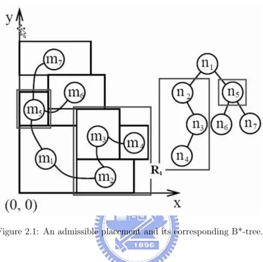
(13) Chapter 2 Large-Scale Circuit Placement with Neighborhood Exchange There were already many approach to solve the large-scale circuit floorplan/placement issue years ago. For example, in floorplanning, there was MB*-tree[10] which extended from B*-tree[1]; in placement such as MPL[12].. 2.1. B*-tree Representation. Given a compacted placement P that can neither move down nor move left called an admissible placement, we can represent it by a unique B*- tree T [1]. (See Figure 2.1(b) for the B*-tree representing the placement of Figure 2.1(a).) A B*-tree is an ordered binary tree whose root corresponds to the module on the bottom-left corner. Using the depth-first search (DFS) procedure, the B*- tree T for an admissible placement P can be constructed in a recursive fashion. Starting from the root, we first recursively construct the left subtree and then the right subtree. Let Ri denote the set of modules located on the right-hand side and adjacent to mi . The left child of the node ni corresponds to the lowest module in Ri that is unvisited. The right child of ni represents the lowest module located above mi , with its x-coordinate equal to that of mi . The B*-tree keeps the geometric relationship between two modules as follows. If 3.

(14) Figure 2.1: An admissible placement and its corresponding B*-tree.. node nj is the left child of node ni , module mj must be located on the right-hand side of mi , with xj = xi + wi . Besides, if node nj is the right child of ni , module mj must be located above module mi , with the x-coordinate of mj equal to that of mi ; i.e., xj = xi . Also, since the root of T represents the bottom-left module, the coordinate of the module is (xroot , yroot ) = (0, 0). Inheriting from the nice properties of ordered binary trees, the B*-tree is simple, efficient, effective, and flexible for handling non-slicing floorplans. It is particularly suitable for representing a non-slicing floorplan with various types of modules and for creating or incrementally updating a floorplan. What is more important, its binary-tree based structure directly corresponds to the framework of a hierarchical scheme, which makes it a superior data structure for multilevel large-scale building module floorplanning/placement.. 4.

(15) 2.2. MB*-tree. In [10], a multilevel floorplanning/placement framework based on the B*-tree representation, called MB*-tree, is presented to handle the floorplanning and packing for large-scale building modules. The MB*-tree adopts a two-stage technique, clustering followed by declustering. The clustering stage iteratively groups a set of modules based on a cost metric guided by area utilization and module connectivity, and at the same time establishes the geometric relations for the newly clustered modules by constructing a corresponding B*-tree for them. The declustering stage iteratively ungroups a set of the previously clustered modules (i.e., perform tree expansion) and then refines the floorplanning/placement solution by using a simulated annealing scheme. In particular, the MB*-tree preserves the geometric relations among modules during declustering, which makes the MB*-tree an ideal data structure for the multilevel floorplanning/placement framework.. 2.3. Performance-Driven Module Perturbation. Those approaches were first bring forth in [11], and promoted in [12]. But they are all about gate array based placement. We first review those approaches in this subsection, then later show our improvement in our framework for efficient largescale circuit placement.. 2.3.1. Unidirectional Circulation Form. Let us consider a board on which every module is placed. Pick one module, denote it by M . Move only module M on the board, while the other modules remain fixed. The wirelength of a signal net does not change, as long as the signal net is not connected to module M . Therefore, we only need to consider the signal nets connected to module M and the sum of the wirelength of these signal nets. This 5.

(16) value is referred to as the wirelength associated with module M . We now define the median of module M. Module M may be placed on m×n different positions (like Figure 2.3). The median of module M is defined as a position where the routing length associated with module M is minimum. Next, sort all the wirelengths associated with module M with respect to the module M position in ascending order. In this order, choose ² elements from the minimum one. The set of these ² positions is defined as the ²-neighborhood for median of module M . Let S be the set of all feasible solutions of this placement and let x be a feasible solution, x ∈ S. Consider the neighborhood of x, denoted by X(x), which is a subset of S. In the first step, x is set to a feasible solution and a search is made in X(x) for a better solution x’ to replace x. This process, which is referred to hereafter as a local transformation, is repeated until no such x’ can be found. A solution x” is said to be a local optimum if x” is better than any other elements of X(x). Many definitions may be considered for the neighborhood of a solution. The set of solutions transformable from x by exchanging not more than λ elements is regarded as the neighboorhood of x. A solution x is said to be λ-optimum if x is better than any other solutions in the neighborhood in this sense. Although the λ-optimum solution gets better as λ increases, the computation time can easily go beyond the acceptable limit when an exhaustive search is performed for large λ. Therefor we present the following method which does not examine all the elements in the neighborhood, nor does it guarantee a λ-optimum solution. However, it is very efficient in the sense that it can be applied for a large value of λ with limited searches in the neighborhood. The search procedure is illustrated along with the search tree shown in Figure 2.2, where each node represents a module and each edge represents a trial transformation. The root node of the tree A is a module chosen to initiate the trial interchange, which. 6.

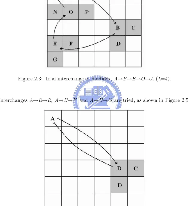
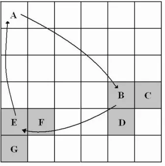
(17) is referred to as the primary module. A path connecting node A and one of the other nodes defines a possible interchange. For example, the path A→B→E→O refers to the trial interchange of four modules, as shown in Figure 2.3. Here, module A is placed on the slot of B, B is placed on E, E on O, and O on A, in a round robin sequence. Although this transformation is a quadruple interchange, it includes a pairwise interchange as a special case, i.e., paths A→B, A→C, and A→D, as shown in Figure 2.4. Value λ indicates the number of modules to be interchanged.. Figure 2.2: The search tree of unidirectional circulation form, and each node represents a module and each edge represents a trial transformation.. The search tree is examined as follows. In this example, ² is fixed as 3. First, module A is interchanged with either one of the modules on trial in the ²-neighborhood of A median (λ = 2). The ²-neighborhood modules are B, C, and D, thus pairwise interchanges between A and B, A and C, and A and D are performed (Figure 2.4). The trial interchange is accepted if it results in the reduction on the total wirelength. If more than one reduction occurs in these transformations, the interchange with the greatest reduction is selected for acceptance. If no interchange contributes to reducing the total routing length, the next step (λ = 3)is initiated. Module A is placed on the slot of B, Then the median of B and its ²-neighborhood are calculated. In this case, the ²-neighborhood module are E, F , and G. Thus 7.

(18) Figure 2.3: Trial interchange of modules, A→B→E→O→A (λ=4).. interchanges A→B→E, A→B→F, and A→B→G are tried, as shown in Figure 2.5.. Figure 2.4: Trial interchange of modules, A→B→A (λ=2).. These trial interchanges are accepted if one of them results in the reduction on the total routing length. Otherwise, we consider the three interchanges of paths 8.

(19) Figure 2.5: Trial interchange of modules, A→B→E→A (λ=3).. A→B→E, A→B→F, and A→B→G, and choose the best one (least total wirelength) for the later tree search. In Figure 2.5, A→B→E is chosen. The solid lines in the tree search shown in Figure 2.2 indicate which searches are to be continued. Broken lines show the searches which are to be terminated. Therefore, no more search efforts are made along paths A→B→F and A→B→G. There is only one solid line under any node, except for root node A. Triple interchanges are performed for the other ²-neighborhood modules, C and D, of root node A. Tree search will be continued following J or L, whereas no search will be accomplished through H, I, K, and M . The tree search is continued, i.e., a path from node A is extended as long as λ is no greater than λ*, which is given as a parameter.. 2.3.2. Permutation Form. This algorithm is based on the concepts from previous form. Assuming all modules except v are fixed in their current locations, we can compute v’s optimal slot locations. Suppose v’s optimal slot location is (r,c) where r is the row index and c is 9.

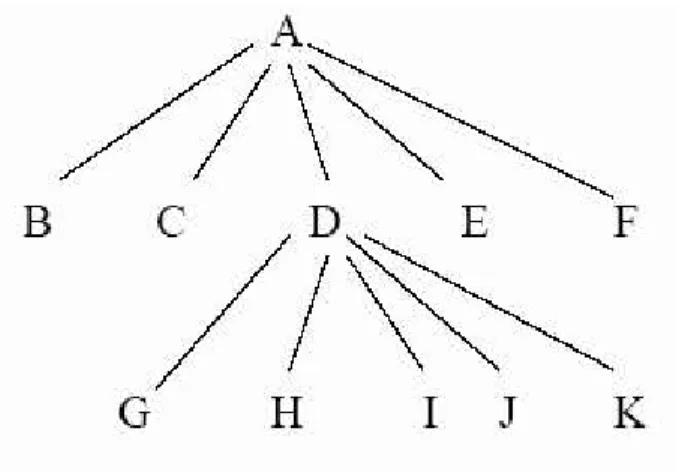
(20) column index in our grid. Modules located in slots at (i,j), where |i-r|+|j-c| 5 ², are called ²-neighbors of module v. For instance, in Figure 2.6, suppose the optimal slot location of module A is occupied by module B. A’s 1-neighbors (² = 1) are {B, C, D, E, F }. Similarly, assuming that D’s optimal slot is taken by G, we say module D’s 1-neighbors are {G, H, I, J, K }.. Figure 2.6: A’s 1-neighbors {B, C, D, E, F } and D’s 1-neighbors {G, H, I, J, K }.. Figure 2.7: Search tree from A.. This algorithm uses a different λ-exchange algorithm from previous form. In unidirectional circulation form, starting from a module v1 , we compute all of its 10.

(21) ²-neighbors. This procedure generates a search tree, each leaf defines a moduleexchange sequence. We use part of the search tree from module A as example, as shown in Figure 2.7. With ²=1 and λ=3, we use the following exchange sequence for leaf K: A→D→K→A, i.e., move module A to D’s slot, move D to K’s slot, and move K to A’s slot. The best module exchange sequence will be chosen, or no exchange is made when the original placement has a smaller cost. This method has two major drawbacks. First, the size of the search tree grows very quickly with slight increase of ² and λ. Second, the module exchange sequence may not be the best possible. Intuitively, moving a module into its ²-neighborhood has a high probability of reducing the objective function value, but in the last step, moving module vλ to the slot of v1 , may not be good in reducing cost. To address these problems, we revise the λ-exchange procedure as follows. Suppose v1 is the first module to be moved. We compute its ²-neighbors and randomly pick one module, say v2 , among these modules. Then for v2 , we compute its ²neighbors, and randomly pick one module, and continue in this fashion until we have λ modules. For the λ modules, we try all of their placement permutations (the total number is λ!) and exchange modules according to the least cost permutation. For example, suppose we pick modules A, D, and K. All six permutations will be tried: no exchange, A↔D, A↔K, D↔K, A→D→K→A, A→K→D→A. The number of solutions we search still goes exponentially with λ, but not with ². The benefit of randomly selecting ²-neighbors of the optimal slot is that it supports multiple passes across the placement region. Experimental results show that unidirectional circulation form algorithm quickly gets stuck at a local minimum, while permutation form algorithm has a higher probability of finding better solutions.. 11.

(22) 2.4. Problem Formulation. The problem we concerned about is described as follows. Let M = {m1 ,m2 ,...,mn } be a set of n rectangular modules. Each module mi ∈ M is associated with a two tuple (hi , wi ), where hi and wi denote the width and height of mi , respectively. The area Ai of mi is given by hi wi . Let N = {n1 ,n2 ,...,nk } be a set of k net. Each net ni ∈ N is a set of modules which are connected together, like {mi1 ,mi2 ,...} ∈ ni . A placement (floorplan) P = {(xi , yi ) | mi ∈ M } is an assignment of rectangular modules mi ’s with the coordinates of their bottomleft corners being assigned to (xi , yi )’s so that no two modules overlap. The objective of placement/floorplanning is to minimize a specified cost metric such as a combination of the area Atot and wirelength Wtot induced by the assignment of mi ’s, where Atot is measured by the final enclosing rectangle of P and Wtot is the summation of half the bounding box of pins for each net. There were already many works that manipulated multilevel or hierarchical approach to disentangle the large scale issue in VLSI years ago. For example, in graph/circuit partitioning such as Chaco[13], hMetis[14], and ML[15]; in placement such as MPL[12]; in routing such as MRS[16], MR[17], and MARS[18]; in floorplanning, there was MB*-tree[10] which extended from B*-tree[1]. Because of the simplicity and identity, we choose B*-tree for easily representing the non-slicing placement and quickly computing the half-perimeter wirelength of nets. Therefore, we decide to keep the multilevel hierarchy and the B*-tree representation of MB*-tree, but replace its simulated annealing refinement method by ²-neighborhood and λ-exchange algorithm for better performance. Because this algorithm combines the MB*-tree and ²-neighborhood and λ-exchange methods, we called our approach MBNE algorithm.. 12.

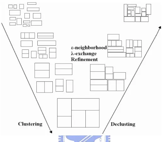
(23) Chapter 3 The MBNE Algorithm In this chapter, we present our MBNE algorithm for multilevel large-scale building module floorplanning/placement. This algorithm adopts a two-stage approach, clustering followed by declustering, by using the B*-tree representation. Figure 3.1 shows the MBNE algorithm flow. The clustering operation results in two types of modules, namely primitive modules and cluster modules. A primitive module m is a module given as an input (i.e., m ∈ M ) while a cluster one is created by grouping two or more primitive modules. Each cluster module is created by a clustering scheme {mi , mj }, where mi (mj ) denotes a primitive or a cluster module. In the following subsections, we give a detailed review on clustering and declustering algorithms in MB*-tree[10] and our refinement approaches in declustering phase to improve the packing results.. 3.1. The Clustering Phase. In this stage, we iteratively group a set of (primitive or cluster) modules until a single cluster is formed (or until the number of cluster modules is smaller than a threshold) based on a cost metric of area and connectivity. The clustering metric is defined by the two criteria: area utilization (dead space) and the connectivity 13.

(24) Figure 3.1: The MBNE algorithm flow. Clustering followed by declustering and using our refinement approaches in declustering phase to improve the packing results.. density among modules. • Dead space: The area utilization for clustering two modules mi and mj can be measured by the resulting dead space sij , representing the unused area after clustering mi and mj . Let stot denote the dead space in the final floorplan P P . We have stot = Atot - mi ∈M Ai , where Ai denotes the area of module mi P and Atot the area of the final enclosing rectangle of P . Since mi ∈M Ai is a constant, minimizing Atot is equivalent to minimizing the dead space stot . • Connectivity density: Let the connectivity cij denote the number of nets between two modules mi and mj . The connectivity density dij between two (primitive or cluster) modules mi and mj is given by dij = cij /(ni + nj ) 14. (3.1).

(25) where ni (nj ) denotes the number of primitive modules in mi (mj ). Often a bigger cluster implies a larger number of connections. The connectivity density considers not only the connectivity but also the sizes of clusters between two modules to avoid possible biases. Obviously, the cost function of dead space is for area optimization while that of connectivity density is for timing and wiring area optimization. Therefore, the metS ric for clustering two (primitive or cluster) modules mi and mj , φ : {mi ,mj }→<+ {0}, is then given by φ({mi , mj }) = αˆ sij +. βK dîj. (3.2). where sîj and K/dîj are respective normalized costs for sij and K/dij , α, β and K are user-specified parameters/constants. Based on φ, we cluster a set of modules into one at each iteration by applying the aforementioned methods until a single cluster containing all primitive modules is formed or the number of modules is smaller than a given threshold (and thus can be easily handled by the classical program). During clustering, we record how two modules mi and mj are clustered into a new cluster module mk . If mi is placed left to (below) mj , then mi is horizontally (vertically) related to mj , denoted by mi →(↑)mj . If mi →(↑)mj , then nj is the left (right) child of ni in its corresponding B*-tree.(See Figure 3.2.) The relation for each pair of modules in a cluster is established and recorded in the corresponding B*-subtree during clustering. It will be used for determining how to expand a node into a corresponding B*-subtree during declustering.. 3.2. The Declustering Phase. We first introduce the metric for refining floorplan/placement solutions. The declustering metric is defined by the two criteria: area utilization (dead space) and the 15.

(26) Figure 3.2: The relation of two modules and their clustering.[10] (a) Two candidate modules mi and mj . (b) The clustering and the corresponding B*-subtree for the case where mi is horizontally related to mj . (c) The clustering and the corresponding B*-subtree for the case where mi is vertically related to mj .. wirelength among modules. • Dead space: Same as that defined in Section 3.1. • Wire length: The wirelength of a net is measured by half the bounding box of all the pins of the net, or by the length of the center-to-center interconnections between the modules if no pin positions are specified. The wirelength for clustering two modules mi and mj , wij , is measured by the total wirelength interconnecting the two modules. The total wirelength in the final floorplan P , wtot , is the summation of the length of the wires interconnecting all modules. Obviously, the cost function of dead space is for area optimization while that of wirelength is for timing and wiring area optimization. Therefore, the metric S for refining a floorplan solution during declustering, ψij :{mi ,mj }→<+ {0}, is then given by ψij = γˆ sij + δ wîj. (3.3). where sîj and w îj are respective normalized costs for sij and wij , and γ and δ are user-specified parameters. The declustering stage iteratively ungroups a set of previously clustered modules (i.e., expand a node into a subtree according to the B*-tree constructed at the 16.

(27) clustering stage) and then refines the floorplan solution based on the ²-neighborhood and λ-exchange method. Figure 3.3 shows the algorithm for declustering a cluster module mk into two modules mi and mj that are clustered into mk at the clustering stage. Without loss of generality, we make mi right to or below mj . In Algorithm Declustering (see Figure 3.3), parent(ni ), right(ni ), and left(ni ) denote the parent, the right child, and the left child of node ni in a B*-tree, respectively. Line 1 updates the parent of nk as that of ni . Lines 2-5 make ni a left (right) child if nk is a left (right) child. Lines 6-13 deal with the case where mi is horizontally related to mj . If mi →mj , then nj is the left child of ni and thus we update the corresponding links in Line 7. Lines 8-10 (11-13) update the links associated the right (left) child of nk . Similarly, lines 14-23 cope with the case where mi is vertically related to mj .. Figure 3.3: The declustering algorithm.[10]. 17.

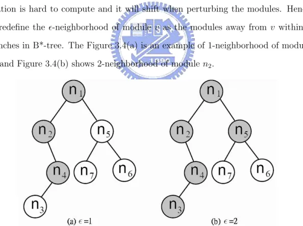
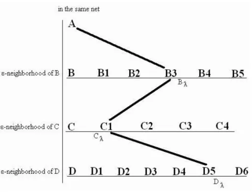
(28) 3.3. Our Refinement Method In Declustering Phase. At all levels of declustering, we apply the ²-neighborhood and λ-exchange method to refine the floorplan for gaining a better solution. This algorithm is inspired by the [11][12] mentioned in Section 2.3, but these two papers are for standard cell based placement. Since we focus on the large-scale circuit placement, we redefine the ² and λ to adjust the B*-tree representation. The original definition of ²-neighborhood of module v in [11] is the modules located in slots at row i, column j where |i-r|+|j-c|5 ² and (r,c) is the optimal slot location of v. But in the non-slicing placement of large-scale circuit, the optimal slot location is hard to compute and it will shift when perturbing the modules. Hence we redefine the ²-neighborhood of module v as the modules away from v within ² branches in B*-tree. The Figure 3.4(a) is an example of 1-neighborhood of module n2 , and Figure 3.4(b) shows 2-neighborhood of module n2 .. Figure 3.4: The definition of ²-neighborhood in our refinement method.. In our refinement algorithm, first we choose a starting module A, and select the module B which in the same net with module A. We then randomly pick the module Bλ in the ²-neighborhood of module B, so we have A and Bλ for 2-exchange now. 18.

(29) Furthermore, we can continue selecting the module C which in the same net with A and B, and randomly pick the module Cλ in ²-neighborhood of module C for 3-exchange. Do this sequence until we have λ modules for λ-exchange. (See Figure 3.5.). Figure 3.5: An example of λ-exchange, λ=4.. After we get all the λ modules, we try all of their placement permutations. Since this is a large-scale circuit placement, modules normally have different heights and widths. Therefore the rotation of modules will affect the placement’s result. The total number of permutations is λ! × 2λ . Finally, we keep the permutation with the lowest cost and start the next turn of refinement.. 3.3.1. Null Module Insertion For Further Movement. The ²-neighborhood and λ-exchange refinement can rotate and/or swap the modules to perturb the placement, but it can not move a module to another place. Thus, we replace one of the λ-exchange modules by null module for permutations. The 19.

(30) null module does not connect to any module, and its height and width are equal to zero. When we decide to use null module by some probability, we insert it to be the replaced λ-exchange module’s child. When a module swap with the null module, it is equivalent moving the module to be the replaced module’s child. Figure 3.6 is an example of null module insertion for refinement.. Figure 3.6: An example of null module insertion for refinement. (a)Insert modele N to replace modele B for swaping. (b)After swap, A→D→C→N →A. (c)Delete module N .. We have applied the null module in the ²-neighborhood and λ-exchange refinement, so we can combine the following three operations to perturb the placement into the lowest cost one. • Op1: Rotate a module. • Op2: Move a module to another place. • Op3: Swap two modules.. 3.4. Floorplanner Flow. The MBNE algorithm integrates the aforementioned three algorithms. We first perform clustering to reduce the problem size level by level and then enter the declustering stage. In the declustering stage, we perform floorplanning for the modules at each level using the ²-neighborhood and λ-exchange algorithm for refinement. 20.

(31) Figure 3.7 illustrates an execution of the MBNE algorithm. For explanation, we cluster three modules each time in Figure 3.7. Figure 3.7(a) lists seven modules to be packed, mi ’s, 1≤i≤7. Figure 3.7(b)-(d) illustrates the execution of the clustering algorithm. Figure 3.7(b) shows the resulting configuration after clustering m5 , m6 , and m7 into a new cluster module m8 (i.e., the clustering scheme of m8 is {{m5 ,m6 },m7 }). Similarly, we cluster m1 ,m2 , and m4 into m9 by using the clustering scheme {{m2 , m4 }, m1 }. Finally, we cluster m3 ,m8 , and m9 into m10 by using the clustering scheme {{m3 , m8 }, m9 }. The clustering stage is done, and the declustering stage begins, in which ²-neighborhood and λ-exchange method are applied to refine the coarse floorplan. In Figure 3.7(e), we first decluster m10 into m3 , m8 , and m9 (i.e., expand the node n10 into the B*-subtree illustrated in Figure 3.7(e)). We then move m8 to the top of m9 (perform Op2 for m8 ) during ²-neighborhood and λ-exchange refinement (see Figure 3.7(f)). As shown in Figure 3.7(g), we further decluster m9 into m1 , m2 , and m4 , and then rotate m2 and move m3 on top of m2 (perform Op1 on m2 and Op2 on m3 ), resulting in the configuration shown in Figure 3.7(h). Finally, we decluster m8 shown in Figure 3.7(i) to m5 , m6 , and m7 , and move m4 to the right of m3 (perform Op2 for m4 ), which results in placement with good quality shown in Figure 3.7(j).. 21.

(32) Figure 3.7: An example of MBNE algorithm.[10]. 22.

(33) Chapter 4 Experimental Results We implement the MBNE algorithm in C++ programming language. The platform is Intel Pentium 4 2.4GHz CPU with 1.5GB memory. We make the comparisons with the MB*-tree algorithm on benchmarks including industry[10], MCNC[19] and GSRC[20] suites for area, wirelength and simultaneous area and wirelength optimizations.. 4.1. Industry with MB*-tree (Area, Wirelength, Area/Wirelength). The circuit industry is a 0.18µm, 1GHz industrial design with 189 modules, 20 million gates and 9,777 center-to-center interconnections. It is a large chip design and consists of three modules with aspect ratios greater than 19 and as large as 36. In each entry of the table, we list the best/average values obtained in ten runs of MBNE and MB*-tree. Table 4.1 shows the results of MBNE compared with MB*-tree. For area optimization, MBNE can obtain a dead space of only 1.99% while MB*-tree results in a dead space of 2.32%. For wirelength optimization, MBNE can obtain a total wirelength of only 53723 mm while MB*-tree requires a total wirelength of 55971 mm. For simultaneous area and wirelength optimization, MBNE can obtain a dead 23.

(34) space of 9.95% and wirelength of 63583 mm while MB*-tree requires 14.45% and 67179 mm.. Package MBNE MB*-tree Package MBNE MB*-tree. Wirelength optimization Area optimization Time Wirelength Time Dead space Area 2 (min) (mm) (min) (%) (mm ) 53723/58585 150.28/150.18 4.00/3.47 671.32/674.57 1.99/2.45 55971/59759 180.45/184.54 3.95/3.84 673.60/679.41 2.32/3.15 Simultaneous area and wirelength optimization Time Dead space Wirelength Area 2 (min) (mm) (%) (mm ) 150.12/150.10 730.70/742.07 9.95/11.30 63583/63956 153.96/159.19 769.10/797.28 14.45/17.37 67179/66407. Table 4.1: Comparisons for area optimization alone, wirelength optimization alone, and simultaneous area and wirelength optimization between MBNE and MB*-tree based on the circuit industry.. 4.2. MCNC - ami49 1-200 with MB*-tree (Area). The ami49 is the largest MCNC benchmark circuit, and we created seven synthetic circuits, named ami49 x, by duplicating the modules of ami49 by x times to test the capability of our algorithm. The largest circuit ami49 200 contains 9800 modules. Table 4.2 shows the result of MBNE compared with MB*-tree. The MBNE obtains 0.3%-1.34% improvement in dead space compared with MB*-tree for the seven ami49 x circuits.. 4.3. GSRC - n100-300 with MB*-tree (Area, Wirelength). The n100, n200, and n300 are the three GSRC benchmark circuit. We used them to compare the MBNE with MB*-tree for area and wirelength optimizations. Table 4.3 shows the number of modules, number of nets, and total area of the GSRC benchmark. 24.

(35) Circuit. #. Total. modules. area. Area. Dead space. Time. Area. Dead space. Time. in dead space. (mm2 ). (mm2 ). (%). (min). (mm2 ). (%). (min). (%). Improvement. MBNE. MB*-tree. ami49. 49. 35.445. 36.46. 2.79. 1.19. 36.22. 2.14. 1.00. 0.65. ami49 4. 196. 141.780. 146.86. 3.46. 6.29. 144.86. 2.12. 5.00. 1.34. ami49 20. 980. 708.908. 732.19. 3.18. 10.21. 727.81. 2.60. 10.08. 0.58. ami49 60. 2940. 2126.724. 2211.75. 3.84. 16.73. 2195.76. 3.14. 15.17. 0.70. ami49 100. 4900. 3544.540. 3704.65. 4.32. 20.47. 3681.56. 3.72. 20.18. 0.60. ami49 150. 7350. 5316.750. 5590.95. 4.90. 26.77. 5560.33. 4.38. 25.58. 0.52. ami49 200. 9800. 7089.808. 7478.55. 5.21. 31.65. 7454.86. 4.91. 30.13. 0.30. Table 4.2: Comparisons for area, dead space, and runtime between MBNE and MB*-tree with the MCNC benchmark.. Table 4.4 shows the results of MBNE compared with MB*-tree. For area optimization, MBNE can obtain dead space of only 1.64%, 2.09% and 2.08% while MB*-tree results in dead space of 2.62%, 2.39% and 2.20%. For wirelength optimization, MBNE can obtain total wirelength of only 110.982 mm, 241.696 mm and 388.162 mm while MB*-tree requires total wirelength of 111.819 mm, 244.233 mm and 391.651 mm.. 4.4. Efficiency with MB*-tree. We choose four circuits from the industry, MCNC, and GSRC benchmark to compare for efficiency between MBNE and MB*-tree algorithm. We set the runtime of MBNE equal to 70% runtime of MB*-tree algorithm for four circuits. Table 4.5 shows the results of area, dead space and runtime of MBNE and MB*-tree. MBNE obtains dead space of 2.34%, 2.11%, 2.89% and 2.32% while MB*-tree requires dead space of 2.32%, 2.62%, 3.18% and 3.84% in these four circuits.. 25.

(36) Circuit n100 n200 n300. # of modules 100 200 300. # of nets 885 1585 1893. Total area (0.001mm2 ) 179.50 175.70 273.17. Table 4.3: The number of modules, number of nets, and total area of the GSRC benchmark.. Area Area n100 (0.001mm2 ) 182.490 MBNE 184.338 MB*-tree Area Area n200 (0.001mm2 ) 179.452 MBNE 180.000 MB*-tree Area Area n300 (0.001mm2 ) 278.964 MBNE 279.310 MB*-tree. optimization Dead space (%) 1.64 2.62 optimization Dead space (%) 2.09 2.39 optimization Dead space (%) 2.08 2.20. Wirelength optimization Time Time Wirelength (min) (mm) (min) 10.03 110.982 5.00 10.89 111.819 5.17 Wirelength optimization Time Time Wirelength (min) (mm) (min) 15.37 241.696 7.00 15.94 244.233 7.78 Wirelength optimization Time Time Wirelength (min) (mm) (min) 20.40 388.162 10.01 21.45 391.651 10.17. Table 4.4: Comparisons for area and wirelength optimization between MBNE and MB*-tree with the GSRC benchmark.. Circuit. #. Total. modules. area. Area. (0.001mm2 ). (0.001mm2 ). Dead space. Improvement. MBNE. MB*-tree Time. Area. Dead space. Time. in time. (%). (min). (0.001mm2 ). (%). (min). (%). industry. 189. 657,984. 673,600. 2.32. 3.95. 673,731. 2.34. 2.77. 29.9. n100. 100. 179.500. 184.338. 2.62. 5.17. 183.365. 2.11. 3.61. 30.2. ami49 20. 980. 708,908. 732,190. 3.18. 10.21. 729,982. 2.89. 7.57. 25.9. ami49 60. 2940. 2,126,724. 2,211,750. 3.84. 16.73. 2,199,793. 3.32. 11.73. 29.9. Table 4.5: Comparisons for efficiency between MBNE and MB*-tree with four benchmark.. 26.

(37) Chapter 5 Conclusion and Future Works In this thesis, we have shown the approaches on the multilevel hierarchical floorplan/placement for large-scale circuits. With the MBNE algorithm, we can choose to optimize area only, wirelength only, or simultaneous area and wirelength with any ratio of the placement. Our MBNE algorithm combines the B*-tree representation and multilevel framework of MB*-tree, and the improved format of ²-neighborhood and λ-exchange refinement method. Experimental results have shown that the MBNE algorithm has better performance compared with the MB*-tree, state of the art floorplanner, in several benchmarks. For future improvement of our placement method, developing the locally perturbation of later declutering level may solve the scalability of increased number of modules. Or we can adopt the ²-neighborhood and λ-exchange refinement method to another framework of algorithm, this may improve its performance.. Acknowledgement We thank Mr. Hsun-Cheng Lee and Prof. Yao-Wen Chang for their MB*-tree platform and industry benchmark.. 27.

(38) Bibliography [1] Y.-C. Chang, Y.-W. Chang, G.-M. Wu, and S.-W. Wu. “B*-trees: A new representation for non-slicing floorplans”. In Proceedings IEEE/ACM Design Automation Conference, pages 458–463, 2000. [2] P.-N. Guo, C.-K. Cheng, and T. Yoshimura. “An O-tree representation of non-slicing floorplan and its applications”. In Proceedings IEEE/ACM Design Automation Conference, pages 268–273, 1999. [3] J.-M. Lin and Y.-W. Chang. “TCG: A transitive closuer graph based representation for non-slicing floorplans”. In Proceedings IEEE/ACM Design Automation Conference, pages 764–769, 2001. [4] J.-M. Lin and Y.-W. Chang. “TCG-S:Orthogonal coupling of P*-admissible representations for general floorplans”. In Proceedings IEEE/ACM Design Automation Conference, pages 842–847, 2002. [5] J.-M. Lin, Y.-W. Chang, and S.-P. Lin. “Corner sequence: A P-admissible floorplan representation with a worst-case linear-time packing scheme”. IEEE Transactions on Very Large Scale Integration (VLSI) Systems, 11(4):679–686, August 2003. [6] H. Murata, K. Fujiyoshi, S. Nakatake, and Y. Kajitani. “Rectangle-packing based module placement”. In Proceedings IEEE/ACM International Conference on Computer-Aided Design, pages 472–479, 1995. 28.

(39) [7] S. Nakatake, K. Fujiyoshi, H. Murata, and Y. Kajitani. “Module placement on BSG-structure and IC layout applications”. In Proceedings IEEE/ACM International Conference on Computer-Aided Design, pages 484–491, 1996. [8] R. H. J. M. Otten. “Automatic floorplan design”. In Proceedings IEEE/ACM Design Automation Conference, pages 261–267, 1982. [9] D. F. Wong and C. L. Liu. “A new algorithm for floorplan design”. In Proceedings IEEE/ACM Design Automation Conference, pages 101–107, 1986. [10] H.-C. Lee, Y.-W. Chang, J.-M. Hsu, and H. H. Yang.. “Multilevel floor-. planning/placement for large-scale modules using B*-trees”. In Proceedings IEEE/ACM Design Automation Conference, pages 812–817, 2003. [11] S. Goto. “An efficient algorithm for the two-dimensional placement problem in electrical circuit layout”. IEEE Transactions on Circuits and Systems, 28(1):12– 18, January 1981. [12] T. F. Chan, J. Cong, T. Kong, and J. R. Shinnerl. “Multilevel optimization for large-scale circuit placement”. In Proceedings IEEE/ACM International Conference on Computer-Aided Design, pages 171–176, 2000. [13] B. Hendrickson and R. Leland. “A multilevel algorithm for partitioning graph”. In Proceedings of Supercomputing, 1995. [14] G. Karypis and V. Kumar. “Multilevel k-way hypergraph partitioning”. In Proceedings IEEE/ACM Design Automation Conference, pages 343–348, 1999. [15] C. J. Alpert, J.-H. Huang, and A. B. Kahng. “Multilevel circuit partitioning”. IEEE Transactions on Computer-Aided Design of Integrated Circuits and Systems, 17(8):655–667, August 1998.. 29.

(40) [16] J. Cong, J. Fang, and Y. Zhang. “Multilevel approach to full-chip gridless routing”. In Proceedings IEEE/ACM International Conference on ComputerAided Design, pages 396–403, 2001. [17] S.-P. Lin and Y.-W. Chang. “A novel framework for multilevel routing considering routability and performance”. In Proceedings IEEE/ACM International Conference on Computer-Aided Design, pages 44–50, 2002. [18] J. Cong, M. Xie, and Y. Zhang. “An enhanced multilevel routing system”. In Proceedings IEEE/ACM International Conference on Computer-Aided Design, pages 51–58, 2002. [19] http://www.cse.ucsc.edu/research/surf/gsrc/mcncbench.html. [20] http://www.cse.ucsc.edu/research/surf/gsrc/gsrcbench.html.. 30.

(41) 作者簡歷王冠中，民國六十七年六月出生於台北市。民國九十年六月畢業於國立交通大學電子工程學系，並於同年八月入伍服役。民國九十二年九月進入國立交通大學電子研究所就讀，從事 VLSI 實體設計方面相關研究。民國九十四年六月取得碩士學位，碩士論文題目為『多層架構的鄰近單元交換方法之大型電路佈局』。.

(42)