在不同色彩空間座標以區域為基礎做彩色影像分割

全文

(1)國立交通大學電機與控制工程學系碩士論文. 在不同色彩空間座標以區域為基礎做彩色影像分割. A Region-Based Segmentation Method of Color Images in Different Color Space. 研究生：王楀鴻指導教授：李祖添. 教授. 中華民國九十四年七月.

(2) 在不同色彩空間座標以區域為基礎做彩色影像分割 A Region-Based Segmentation Method of Color Images in Different Color Space. 研究生：王楀鴻. Student：Yu-Hung Wang. 指導教授：李祖添教授. Advisor：Dr. Tsu-Tian Lee. 國立交通大學電機與控制工程系碩士論文. A Thesis Submitted to Department of Electrical and Control Engineering College of Electrical Engineering and Computer Science National Chiao Tung University in partial Fulfillment of the Requirements for the Degree of Master in Electrical and Control Engineering June 1997 Hsinchu, Taiwan, Republic of China. 中華民國九十四年七月.

(3) 在不同色彩空間座標以區域為基礎做彩色影像分割. 研究生：王楀鴻. 指導教授：李祖添博士. 國立交通大學電機與控制工程系碩士班摘要本論文的內容將探討彩色影像分割的方法，基本的影像分割方法有四種： (一)統計取閥值 (二)以邊緣為基礎 (三)以區域為基礎 (四)以物理性質為基礎，每個方法都有其優缺點，而彩色影像的分割就是結合基本影像分割的理論再加上色彩的資訊，使得可以從原來處理黑白影像進而到彩色影像。而色彩的資訊表示方式可以用許多不同的色彩空間座標來表示，同樣的，每個色彩空間座標都有其優缺點，所以本文採用以區域為基礎的分割法包含區域成長和區域合併，加上運用 3-D 聚集及鬆弛標記的方法來做彩色影像分割，來減少只使用區域為基礎分割的缺點，並將其在不同的色彩空間座標實現，找出最適合此提出的演算法的色彩空間，並加以比較。此提出的演算法的優點為其考慮了影像上空間的資訊和其色彩的資訊並且減少了雜訊對我們處理的影響，同時應用在適當的色彩空間下，可以提高色彩分割的準確率，減少影像在實際生活中，陰影和光線的影響所造成分割的不準確，進而使之後影像的後處理產生錯誤。本文首先將介紹各種基本的影像分割的方法和所常用的色彩空間座標，然後介紹此所提出的演算法所使用的理論，如：3-D 聚集、鬆弛、標記和本文所使用來判斷區域合併的條件，並將此區域合併演算法的流程圖秀出。整個系統的流程圖包含區域成長和區域合併都會列出使讀者了解。最後由實驗結果來驗證比較在何種色彩空間座標下，有最好的分割效果，和最好的雜訊和閥值的容忍度及處理速度和峰值的訊號雜訊比。. i.

(4) A Region-Based Segmentation Method of Color Images in Different Color Space Student : Yu-Hung Wang. Adviser : Dr. Tsu-Tian Lee. Department of Electrical and Control Engineering, National Chiao Tung University ABSTRACT A color image segmentation method is presented in this thesis. There are four basic methods of image segmentation: (1) histogram thresholding approaches; (2) edge based approaches; (3) region based approaches; (4) physical based approaches. Each method has its own advantages and disadvantages. The color image segmentation is combined with these basic image segmentation methods and color information in the image. So we can process color images. There are also many color space to represent color information. Similarly, each color space has its own virtues and drawbacks. We adopt region based approaches to segment color image in the thesis. We use 3-D clustering and relaxation labeling to do region growing to reduce the shortcomings of the region based approaches, and we realize this algorithm in the different color space to find the most suitable color space for this algorithm and we compare them. The advantages of this proposed algorithm are color information and spatial relation in the image. We also reduce the noise effect. In the suitable color space, we can improve the accuracy of color image segmentation because we reduce the shadow and highlights effects which may happen in the real world image. So the error in the post image process will be decreased. In the thesis, we will introduce these basic image segmentation approaches and several frequently used color space first. Then the methods in this proposed algorithm will be bring up such as 3-D clustering, relaxation, labeling and the flowchart of region merging process including the determination of the process doing or not. The whole system including region growing process and region merging process will be show in detail to tell the reader to know this proposed algorithm. Finally, the experiment results will test and verify this proposed algorithm and prove which color space has the better color image segmentation performance and suitable for this algorithm. The comparison between every color space will be told about. The tolerance of the noise and threshold, and peak signal and noise ratio will be shown to illustrate.. ii.

(5) 誌. 謝. 在此由衷的感謝恩師李祖添教授在研究所的悉心指導和鼓勵，從老師身上學得不僅是專業領域的知識，更學習到做學問的方法，使我受益良多。也感謝鄭銘揚老師的教導，使我擁有札實的基礎。同時感謝陳彥霖學長在論文研究上所提供寶貴的意見和指導，使我論文更加完善，也感謝有著共同革命情感的實驗室的同學們在學業上的討論和生活上的照顧。最後僅以本論文獻給我的父母、家人及所有關心我的師長與朋友們，和他們共享這份成果與榮耀。. iii.

(6) 目錄摘要 ....................................................................................................................................... i ABSTRACT .......................................................................................................................... ii 誌謝 ..................................................................................................................................... iii 目錄 ..................................................................................................................................... iv List of Figures ....................................................................................................................... v List of Tables ........................................................................................................................ vi Chapter 1. Introduction .......................................................................................................... 1 1.1 Background.............................................................................................................. 2 1.2 Organization of the thesis ....................................................................................... 10 Chapter 2. Color Space .........................................................................................................11 2.1 Overview ................................................................................................................11 2.2 Linear Transformation............................................................................................ 13 2.2.1 YIQ Color Space ......................................................................................... 13 2.2.2 I1I2I3 Color Space ........................................................................................ 13 2.3 Nonlinear Transformation....................................................................................... 14 2.3.1 nRGB (Normalized RGB) Color Space........................................................ 14 2.3.2 HSI Color Space.......................................................................................... 15 2.3.3 Munsell Color Space.................................................................................... 18 Chapter 3. Proposed System Model for Color Segmentation ................................................ 21 3.1 Overview ............................................................................................................... 21 3.2 System Model ........................................................................................................ 22 3.3 Smooth and Cluster ................................................................................................ 24 3.4 Labeling ................................................................................................................. 26 3.4.1 Relaxation ................................................................................................... 28 3.4.2 Relaxation Labeling..................................................................................... 33 3.5 Region Merging ..................................................................................................... 35 3.6 The Proposed Algorithm......................................................................................... 36 Chapter 4. Experimental Results .......................................................................................... 41 4.1 Experiment Results ................................................................................................ 41 4.2 Comparison with Different Color Space ................................................................. 48 Chapter 5. Conclusion and Future Work............................................................................... 51 5.1 Conclusion ............................................................................................................. 51 5.2 Future Work ........................................................................................................... 52 References ........................................................................................................................... 53. iv.

(7) List of Figures Fig. 2.1 RGB color space represented in a 3-dimensional cube ............................................ 12 Fig. 2.2 HSI color space....................................................................................................... 16 Fig. 2.3 The HSI triangle shown in the RGB color cube . ..................................................... 17 Fig. 2.4 Minsell color space . ............................................................................................... 18 Fig. 3.1 Commonly used color image segmentation approaches . ......................................... 22 Fig. 3.2 Flowchart of the proposed algorithm. ...................................................................... 23 Fig. 3.3 Example for smooth function. ................................................................................. 25 Fig. 3.4 4-adjacent and 8-adjacent........................................................................................ 26 Fig. 3.5 Scene labeling example........................................................................................... 29 Fig. 3.6 Inconsistent labeling. .............................................................................................. 30 Fig 3.7 Discrete relaxation: (a) all labels assigned to each object; (b) locally inconsistent labels are removed; (c) final consistent labeling. ................................................................ 31 Fig 3.8 A relaxation labeling step. ........................................................................................ 34 Fig 3.9 Flowchart of proposed region growing by relaxation labeling algorithm. ................. 39 Fig 4.1 Origin input color image (a) fruit (b) plane (c) pool (d) baboon................................ 41 Fig 4.2 Output resulting fruit image. (a) RGB (b) YIQ (c) I1I2I3 (d) nRGB (normalized RGB) (e) HSI (f) HVC......................................................................................... 42 Fig 4.3 Output resulting plane image. (a) RGB (b) YIQ (c) I1I2I3 (d) nRGB (normalized RGB) (e) HSI (f) HVC......................................................................................... 42 Fig 4.4 Output resulting pool image. (a) RGB (b) YIQ (c) I1I2I3 (d) nRGB (normalized RGB) (e) HSI (f) HVC......................................................................................... 43 Fig 4.5 Output resulting baboon image. (a) RGB (b) YIQ (c) I1I2I3 (d) nRGB (normalized RGB) (e) HSI (f) HVC......................................................................................... 43. v.

(8) List of Tables Table 1.1 Comparisons of segmenting techniques. ................................................................. 8 Table 2.1 The correspondence between the human color perception and the NBS distance. .. 20 Table 4.1 Comparisons of different color space of Fig. 4.2................................................... 47 Table 4.2 Comparisons of different color space of Fig. 4.3................................................... 47 Table 4.3 Color space conclusions of these four cases input image....................................... 48 Table 4.4 (a) Comparisons of merits and shortcoming for different color spaces................... 48 Table 4.4 (b) Comparisons of various performances for different color spaces. .................... 49. vi.

(9) Chapter 1. Introduction. Chapter 1. Introduction People are interested in digital image processing methods that come from two important applications: one is to modify image information to let people understand clearly what it is, and the other is to let the image scene data be recognized by computer automatically. So the most significant work of image processing is to transform images including many signals and characters to the information which has its actuality meaning. Many research have been published [1] [2]. The image segmentation is to extract objects and components detail, and it is a very important image process technique in many image analyses and implications. In many applications, not all of signals are needed to deal with. The image segmentation is employed to extract meaningful data in image for effective processing image analysis. The principal works of image segmentation are extracting different composing objects or separating objects from the background by information in the image. It separates each object single-handed and analyzes effective information in order to get each character. The traditional image segmentation techniques are used in monochrome image and gray level image. Its principle is based on two essential properties of gray level which are discontinuity and similarity. There are two basic methods, namely, the region-based method and edge-based method, among two essential properties of gray level. The region-based method is using gradient image to find the boundaries of the objects. These boundaries separate the image into several different regions. But this method is not good when the intensity is not continuous. The edge-based method set all pixels in the image with different regions. This method is sensitive to noise and intensity contrast. It has long been recognized that human eye can discern thousands of color shades and intensities but only two-dozen shades of gray. It is quite often when the objects cannot be extracted using gray scale but can be extracted using color information. Compared to gray scale, color provides information in addition to intensity. Color is useful or even necessary for 1.

(10) Chapter 1. Introduction. pattern recognition and computer vision. Also the acquisition and processing hardware for color images have become more available and accessible to deal with the computational complexity caused by the high dimensional color space. Hence, color image processing has become increasingly more practical. In the thesis, the 3-D clustering and relaxation labeling method are employed to segment color images. The proposed method can avoid the seed points choosing for region growing and reducing noise influence, because the region is based on the similarity of color. This assumption often makes it difficult for any algorithms to separate the objects with highlights, shadows, shadings or texture which cause inhomogeneity of colors of the objects’ surface. So we use several color space to overcome these disadvantages. Then the algorithm will have both advantages. And the final results will retain most important information of origin color image. The trivial color and region will be eliminated. It will be separated and recognized easily and will be transferred with low cost.. 1.1 Background In this section, we will introduce several basic theorems [3] for color image segmentation. For segmentation of color images, the techniques can roughly be categorized into the following four classes [4]: (1) histogram thresholding approaches; (2) edge based approaches; (3) region based approaches; and (4) physics based approaches. A segmentation method may be one of them or a combination of two or more of the mentioned classes. (1) Histogram thresholding is one of the widely used techniques for monochrome image segmentation [5]. It assumes that images are composed of regions with different gray level ranges. The histogram of an image can be separated into a number of peaks, each corresponding to one region, and there exists a threshold value corresponding to valley between the two adjacent peaks. Gray level thresholding is the simplest segmentation process. 2.

(11) Chapter 1. Introduction. Many objects or image regions are characterized by constant reflectivity or light absorption of their surface. A threshold can be determined to segment objects and background. Thresholding is computationally inexpensive and fast. It is the oldest segmentation method and is still widely used in simple applications. It can easily be implemented in real time. A complete segmentation of an image R is a finite set of regions R1, …, Rs,. R =.  S. Ri. i=1. Ri  R j = ∅. i≠j. (1.1). Complete segmentation can result from thresholding in simple scenes. Thresholding is the transformation of an input image f to an output segmented binary image g as follows: g( i, j) = 1. for f( i, j) ≧ T. g( i, j) = 0. for f( i, j) < T. (1.2). where T is the threshold, g( i, j) = 1 for image elements of objects, and g( i, j) = 0 for image elements of the background. The basic thresholding algorithm is shown below: Basic thresholding algorithm: Search all the pixels f( i, j) of the image f. An image element g( i, j) of the segmented image is an object pixel if f( i, j) ≧ T, and is a background pixel otherwise.. If objects do not overlap each other, and if their gray-levels are clearly distinct from background gray levels, thresholding is a suitable segmentation method. There are many thresholding algorithms. How to choose a proper threshold is shown in detail in [6]. As for color images, the situation is different from monochrome image because of multi-features. Multiple histogram thresholding divided color space by thresholding each component histogram. Since the color information is represented by tristimulus R, G, and B color space or their linear or nonlinear transformations, representing the histogram of a color image in a 3-dimensional array and selecting threshold in this histogram is not a trivial job [7]. The advantage of a histogram thresholding technique is that it does not need a priori information 3.

(12) Chapter 1. Introduction. of the image. One of the disadvantages of the histogram-based technique is it can’t guarantee that regions are continuous if it does not consider the spatial details. This problem can be solved by a combination of a histogram-based method and other segmentation methods [8]. (2) Edge based detection is another approach to image segmentation. It is extensively utilized for gray level image segmentation which is based on the detection of discontinuity in gray level trying to locate points with abrupt changes in gray level. Edge detection techniques are usually classified into two categories: sequential and parallel [2] [9]. A parallel edge detection technique means that the decision of whether or not a set of points are on an edge is not dependent on whether other sets of points lie on an edge or not. One technique is high emphasis spatial frequency filtering. Since high spatial frequencies are associated with sharp changes in intensity, one can enhance or extract edges by performing high pass filtering using the Fourier operator. The problem here is how to design a relevant filter. There are many types of parallel differential operators such as Roberts, Sobel, and Prewitt operators which are called the first-difference operators, and the Laplacian operator is called the second-difference operator. The main differences between these operators are the weights assigned to each element of the mask. These operators require that there is a distinct change in gray level between two adjacent points and only very abrupt edges between two regions could be detected. They cannot detect ill-defined edges that are formed by a gradual change in gray level across the edge. Since the computation is based on a small window, the result is quiet susceptible to noises. The noise may cause an edge presence in locations where there is no border and no edge presence where a real border exists. Sequential edge detection means that the result at a point is dependent on the result of the previously examined points. There are a number of sequential techniques utilizing heuristic search and dynamic programming. The performance of a sequential edge detection algorithm will depend on the choice of a good initial point and it is not easy to define a termination criterion. In a monochrome image, edge is defined as a discontinuity in the gray level and can be 4.

(13) Chapter 1. Introduction. detected only when there is a difference of the brightness between two regions. However, in color images, the information about edge is richer than in monochrome case. For example, edges between two objects with the same brightness but different hue can be detected in color images [10]. So an edge should be defined by a discontinuity in a three-dimensional color space in a color image. There are three alternatives for the definition of a color edge [11]: (i) Define a metric distance in some color space and use discontinuities in the distance to determine edges. This makes color edge detection still be performed in 1-D space. Hence the result cannot be expected to be better than that achieved by edge detection in an equivalent monochrome image. (ii) Regard a color image as composed of three monochrome images formed by the three color components, respectively, and perform gray level edge detection on these three images separately. Then the edges detected in the three images might be merged by some specified procedures. This is still essentially a gray level edge detection technique and may be unsatisfactory in some cases, for example, when gradient edge detectors are employed, the three gradients for one pixel may have the same strength but in opposite directions [12] [13]. (iii) Impose some uniformity constraints on the edges in the three color components to utilize all of the three color components simultaneously, but allow the edges in the three color components to be largely independent. Actually, these constraints directly affect the computation of the three color components which makes definition (iii) essentially different from definition (ii). However, edge based detection for image segmentation has difficulties because it does not work well with images in which the edges are ill-defined or where there are too many edges, and it is difficult to link edges into closed boundaries. It can only provide useful information about the region boundaries for the higher level systems. It is possible to obtain a good segmentation result with other approaches, such as region based segmentation combine with edge detection to complete the segmentation tasks. (3) Region based approaches including region growing, region splitting, region merging 5.

(14) Chapter 1. Introduction. and their combination attempt to separate regions on the basis of a homogeneity predicate defined on groups of connected pixels [14]. The regions must satisfy the following conditions:. H ( Ri ) = TRUE. i = 1, 2, …, S. H ( Ri  R j ) = FALSE i≠j,. Ri adjacent to Rj. (1.3). where S is the total number of regions in an image and H(Ri) is a homogeneity evaluation of the region Ri. Resulting regions of the segmented image must be homogeneous. Homogeneity is an important property of regions, and is used as the main segmentation criterion in region based approaches, whose basic idea is to divide an image into zones of maximum homogeneity. The criteria for homogeneity can be based on gray level, color, texture, and etc. In the region growing approach, a seed region is first selected then expanded to include all homogeneous neighbors and this process is repeated until all pixels in the image are classified. Region growing techniques are generally better in noise images where borders are extremely difficult to detect. A problem with region growing is its inherent dependence on the selection of the seed region and the order in which pixels and regions are examined. In the region splitting approach, the initial seed region is simply the whole image. If the seed region is not homogeneous, it is usually divided into four squared sub-regions which become new seed regions. This process is repeated until all sub-regions are homogeneous. The major disadvantage of region splitting is that the resulting image tends to mimic the data structure used to represent the image and comes out too square. The region merging approaches are often combined with region growing or region splitting to merge the similar regions for making a homogeneous region as large as possible. These techniques work best on images with an obvious homogeneity criterion and tend to be less sensitive to noise because homogeneity is typically determined statistically. They are better than thresholding by taking into account both feature space and the spatial relation between pixels simultaneously. However, all region based approaches are by nature sequential, and another problem with 6.

(15) Chapter 1. Introduction. these techniques is their inherent dependence on the selection of seed region and the order in which pixels and regions are examined. The other disadvantage is that they are more expensive in computing time. But the region based approach is widely used in color image segmentation because it considers the color information and spatial details at the same time. It is a quiet strong point. (4) Physics based segmentation approaches aim at solving this problem by employing physical models to locate the objects’ boundaries while eliminating the spurious edges of shadow or highlights in a color image. Two models, the “dichromatic reflection model” [15] and the “approximate color-reflectance model (ACRM)” [16] are the most common ones. Reflection is highly related to the nature of the materials. Reference [16] divided materials into different classes: optically homogeneous materials like metals, glass and crystals, and optically inhomogeneous materials such as plastics, paper, textiles and paints. Usually it is very helpful to identify or classify the material in the scene of an image before the algorithm is applied. For example, we should distinguish metals from dielectrics since they interact with lights in different ways and require different algorithms for image understanding. Reference [15] created a method to determine the amount of interface reflection and body reflection in a color image pixel by pixel and represented an algorithm for analyzing color values which is very useful in color image understanding based on “dichromatic reflection model.” “ACRM” [16] demonstrated the independence of the spectral composition and geometrical scaling of the light reflected. This model is consistent with dichromatic reflection model when the materials are inhomogeneous dielectrics. The existing physics based models are efficient only in image processing for the materials whose reflection properties are know and easy to model. There are too many rigid assumptions of these physics models regarding the material type, the light sources and illumination. These conditions may not be satisfied in the real world. Therefore, these models can be used only in a very limited scope of applications. The comparisons of these 7.

(16) Chapter 1. Introduction. segmentation techniques are tabled below [3]: Table 1.1 Comparisons of segmenting techniques. Segmentation. Method description. Advantages. Disadvantages. Requires that the histogram of an image has a number of peaks, each corresponds to a region and use its valley to segment the regions.. It does not need prior information of the image. For a wide class of images satisfying the requirement, this method works very well with low computation complexity, it is the fastest.. (1) Does not work well for an image without any obvious peaks or with broad and flat valleys. (2) Does not consider the spatial details, so cannot guarantee that the segmented regions are contiguous.. Based on the detection of discontinuity, normally tries to locate points with more or less abrupt changes in gray level. Usually classified into two categories: sequential and parallel.. Edge detecting technique is the way in which human perceives objects and works well for images having good contrast between regions.. (1) Does not work well with images in which the edges are ill-defined or there are too many edges. (2) It is not a trivial job to produce a closed curve or boundary. (3) Less immune to noise than other techniques.. Group pixels into homogeneous regions. Including region growing, region splitting, region merging or their. Work best when the region homogeneity criterion is easy to define. They are also more noise immune than edge detection. (1) Are by nature sequential and quite expensive both in computation time and memory.. technique Histogram thresholding. Edge based approaches. Region based approaches. 8.

(17) Chapter 1. Introduction. Physics based approaches. combination.. approach. It considers both the color information and spatial details at the same time.. (2) Region growing has inherent dependence on the selection of seed region and the order in which pixels and regions are examined. (3) The resulting segments by region splitting appear too square due to the splitting scheme.. Employing physical models to locate the objects’ boundaries while eliminating the spurious edges of shadow or highlights in a color image. “Dichromatic reflection model” and “approximate color reflectance model” are the most common ones.. It is very helpful to identify and classify the material in the scene of an image before the algorithm is applied. It is efficient only in image processing for the materials whose reflection properties are known and easy to model.. There are too many rigid assumptions of these physics models regarding the material type, the light source and illumination. These conditions may not satisfy in the real world. It is very limited used.. As mentioned above, each technique has its own advantages and disadvantages for separating regions in color image. Some disadvantages of one technique can be overcome by the advantages of other techniques. So if we combine several techniques together properly, maybe we can get a better segmentation result. In this thesis, we combine several segmented method like clustering method for smoothing, which is pre-processing stage of a region based approach, relaxation labeling for region assignment of the pixels, and addition to proper color space to get the better results. In our case, the outcome of a relaxation step can be viewed as a 9.

(18) Chapter 1. Introduction. relaxation of the constraint of the triangle inequality which is much different from classical probabilistic relaxation schemes. The computation complexity of the proposed algorithm is lower than those of other methods.. 1.2 Organization of the thesis The remainder of this thesis is organized as follows. In Chapter 2, we will introduce all color space we use in the thesis in order to eliminate the disadvantages of region with highlights and shadows. Each color space will be described in detail including its advantages and disadvantages, and its transformation whether linear or nonlinear from the original color space RGB. All of the color space will be used in the proposed algorithm. In Chapter 3, the proposed algorithm, region growing by relaxation labeling, will be shown. It is the core of the thesis. The procedures of the algorithm will be brought up sequentially and each method we used in the system will also be introduced in detail and systematically including cluster method, labeling, relaxation, region merging, and etc. The overall system flowchart will be shown in the last of the chapter. In Chapter 4, the experiment results of the proposed algorithm will be discussed. We use public commonly used image to test this algorithm. And we will compare all of the color space we use in the algorithm to show its advantages and shortcomings. Finally, in Chapter 5, the conclusions and the future work will be given.. 10.

(19) Chapter 2. Color Space. Chapter 2. Color Space 2.1 Overview Image segmentation is the first step in image analysis and pattern recognition. It is a critical and essential component of image analysis and pattern recognition system, is one of the most difficult tasks in image processing, and determines the quality of the final result of analysis. In order to get better performance in color image segmentation, we use several color space to test which one can get better result and is more robust against noise and shadow in the same algorithm. There are many existing color space for arranging and describing color, such as RGB, YIQ, YUV, I, nRGB, HIS, CIE, Munsell, etc.[17][18]. Each pixel in an image is usually expressed by its R, G, and B values. However, the values of RGB are sometimes not suitable for color processing and we need to do some transformation to convert the RGB color space to some other suitable color space. In this chapter, we will review several color spaces which have been used in my research to see which one can provide better experiment results. Color is perceived by humans as a combination of tristimuli red (R), green (G), and blue (B) which are usually called three primary colors. From R, G, B representation, we can derive all colors in the world. R, G, B components can be obtained through three separate filters based on the following equations:. R = ∫ E (λ ) S R (λ )d λ λ. ( 2.1). G = ∫ E (λ )SG (λ )d λ λ. ( 2.2). B = ∫ E (λ ) S B (λ )d λ λ. ( 2.3). where SR, SG, SB are the color filters on the incoming light or radiance E(λ), and λ is the wavelength. The RGB color space can be geometrically represented in a 3-dimensional cube shown in Fig.2.1 [19]. The coordinates of each point inside the cube represent the values of red, green, and blue components, respectively. The laws of colorimetry [20] are: (1) any color can 11.

(20) Chapter 2. Color Space. be created by these three colors and the combination of the three colors is unique; (2) if two colors are equivalent, they will be again equivalent after multiplying or dividing the three components by the same number; and (3) the luminance of a mixture of colors is equal to the sum of the luminance of each color.. Fig. 2.1 RGB color space represented in a 3-dimensional cube [19].. RGB is the most commonly used model for the television system and pictures acquired by digital cameras. It is suitable for color display, but not good for color scene segmentation and analysis because of the high correlation among the R, G, B components [5]. By high correlation, we mean that if the intensity changes, all the three components will change accordingly. Also, the measurement of a color in RGB space does not represent color differences in a uniform scale. Hence, it is impossible to evaluate the similarity of two colors from their distance in RGB space. So there are some linear transformations and nonlinear transformations to transfer the 12.

(21) Chapter 2. Color Space. RGB color space to other color spaces for improving the disadvantage of RGB color space.. 2.2 Linear Transformation The linear transformation is that the new color spaces are obtained by RGB color space with linear transformation. They both have linear relation and comply with linear algebra properties. The linear transformation needs less computation time than nonlinear ones, which makes the linear systems more preferable to nonlinear systems.. 2.2.1 YIQ Color Space YIQ is used to encode color information in TV signal for American system. It is obtained from the RGB model by a linear transformation:. 0.114   R   Y   0.299 0.587       I  =  0.596 −0.274 −0.322   G   Q   0.211 −0.253 −0.312   B       Where 0≦R≦1 , 0≦G≦1 , 0≦B≦1 .. ( 2.4). The Y component, a measure of the luminance of the color, is a likely candidate for edge detection in a color image. The I and Q components jointly describe the hue and saturation of the image [21]. The YIQ space can partly get rid of the correlation of the red, green and blue components in an image.. 2.2.2 I1I2I3 Color Space Karhunen-Loeve [22] transfer R, G and B to a effective color features as follows:. I1 = ( R + G + B ) / 3. ( 2.5). I 2 = ( R − G) / 2. ( 2.6). 13.

(22) Chapter 2. Color Space. I 3 = (2G − R − B ) / 4. ( 2.7). In [22] claimed that I1I2I3 was more effective in terms of the quality of segmentation and the computational complexity of the transformation. In order to reduce the complexity of I1I2I3, we transfer this color space to I2’ and I3’ color spaces. We can just use I1 Eq. (2.5) and I2’ Eq. (2.8) or I1 and I3’ Eq (2.9) to segment color image. The transform equations are as follows:. I2 ' = (R − B). ( 2.8). I3 ' = (2G − R − B) / 2. ( 2.9). It also can get reduce correlation with other axis.. 2.3 Nonlinear Transformation In this section, we will introduce the new color spaces which are transferred by nonlinear transformation.. 2.3.1 nRGB (Normalized RGB) Color Space The normalized color space is formulated as:. r = R /( R + G + B ). ( 2.10). g = G /( R + G + B). ( 2.11). b = B /( R + G + B ). ( 2.12). Since r + g + b = 1, when two components are given, the third component can be determined. We may use only two of three components. They can represent the real color information of an image and they are independent of the brightness of the image which is one of the advantages of the normalized RGB color system [23]. Because for color image segmentation, we need to make it is desired that colors be independent of the change in lighting intensities. Furthermore, it is more convenient to represent the color plane since the color values 14.

(23) Chapter 2. Color Space. are set to a narrow limitation. An obvious shortcoming of normalized RGB is that the normalized RGB colors are very noisy if they are under low intensities, because they are transferred by nonlinear transformation from RGB color space. And normalization reduces the sensitivity of the distribution to the color variable. But it is relatively robust to the change of the illumination.. 2.3.2 HSI Color Space The HSI ( hue-saturation-intensity) system, which is more intuitive to human vision [3], is another commonly used color space in image processing. And it separates color information of an image from its intensity information. Color information is represented by hue and saturation values, while intensity, which describes the brightness of an image, is determined by the amount of the light. Hue represents basic colors. It is determined by the dominant wavelength in the spectral distribution of light wavelengths. So we can segment objects with different colors by hue only. Since hue is independent on intensity values, it is especially efficient when the images have non-uniform illumination such as shade. The saturation is a measure of the purity of the color. It signifies the amount of white light mixed with the hue. The formulas for RGB to HSI are: H = arctan(. 3(G − B) ) ( R − G ) + ( R − B). ( 2.13). min( R, G , B) I ( R + G + B) I= 3. S = 1−. ( 2.14) ( 2.15). Where the hue is undefined if the saturation is zero, and the saturation is undefined when the intensity is zero. The HSI color space can be described geometrically as in Fig. 2.2. Hue is considered as an angle between a reference line and the color point in RGB space. The range of the hue values is from 0o to 360o and each degree represents its owned color. The saturation 15.

(24) Chapter 2. Color Space. component represents the radial distance from the cylinder center. The nearer the points is to the center, the lighter is the color. Intensity is the height in the axis direction. The axis of the cylinder describes the gray levels. For instance, zero (minimum) intensity is black, and full (maximum) intensity is white. Each slice of the cylinder perpendicular to the intensity axis is a plane with the same intensity.. Fig. 2.2 HSI color space. 16.

(25) Chapter 2. Color Space. Fig. 2.3 The HSI triangle shown in the RGB color cube [19].. The HSI color system has a good capability of representing the colors of human perception, because human vision system can distinguish different hues easily, whereas the perception of different intensity or saturation does not imply the recognition of different colors. And segmentation in the 1-D hue space is computationally less expensive than in the 3-D RGB space. One of the disadvantages of this color space is that hue has a non-removable singularity near the axis of the color cylinder, where a slight change of input R, G and B values can cause a large jump in the transformed values. The singularities may create discontinuities in the representation of colors [20]. Also, if the intensity of the color lies close to white or black, hue and saturation play little role in distinguishing colors. The relationship between RGB color space and HSI color space is shown in Fig. 2.3.. 17.

(26) Chapter 2. Color Space. 2.3.3 Munsell Color Space Munsell color system is one of the earliest methods to specify colors. It was created in 1969 [24] and is the best in simulating the human color vision. The Munsell system describes all possible colors in terms of its three coordinates, Munsell Hue, Munsell Value, Munsell Chroma. Figure 2.4 describes the Munsell color space. It can be represented by a cylindrical coordinate system consisting of H, V and C similar to the HIS space.. Fig. 2.4 Minsell color space [3].. There are five colors regarded as the major hues, red (R), yellow (Y), green (G), blue (B) and purple (P). The combinations of colors: YR, GY, BG, PB, and RP are five half-way hues. The hue circle is divided equally into 100 parts with the five major hues and the five halfway hues located on the circle with equal spaces. All hue values are arranged on the hue circle. Munsell value (V) describes the lightness of a color. It defines the value of black as 0 and the value of white as 10. An equation describes the relationship between V and Luminance Y is. Y = 1.2219V − 0.23111V 2 + 0.23951V 3 − 0.021009V 4 + 0.0008404V 5 18. ( 2.16).

(27) Chapter 2. Color Space. Chroma (C) is like the saturation component in the CIE representation. It describes the purity of a color. When C is equal to zero, it is an achromatic color. A color in the Munsell color system can be written as HV/C. For instance, 5R5/10 stands for that the Munsell Hue is 5R, the Munsell Value is 5, and the Munsell Chroma is 10. Nevertheless, it is impossible to calculate color difference of two colors by such representation. We have to convert such representation into real numbers. So we use the hue, value, chroma space ( HVC color space) instead of the Munsell color space. The HVC color space is a variant of the Munsell color space. It expresses colors in terms of tri-attributes of human color perception [25]. In essential, the HVC color space is the same as the Munsell color system, so the HVC color space also gives the best performance for experiments with variety of color spaces [26]. The following is the color transformation of RGB to HVC [27]:.  xc  0.620 0.178 0.204   R   y  = 0.299 0.587 0.114  G        zc  0.000 0.056 0.942   B . ( 2.17). M1 = f ( xc ) − f ( y ). ( 2.18). M 2 = 0.4 ( f ( zc ) − f ( y ) ). ( 2.19). H3 = f ( y ). ( 2.20). Where f ( u ) =. 18.51u 5.146u   u + 17.58  1 +   u + 30.07 . ( 2.21). S1 = ( 8.880 + 0.966 cos θ ) M 1. ( 2.22). S2 = ( 8.025 + 2.558cos θ ) M 2. ( 2.23). Where θ = arctan. M2 M1. ( 2.24). Finally, we have. 19.

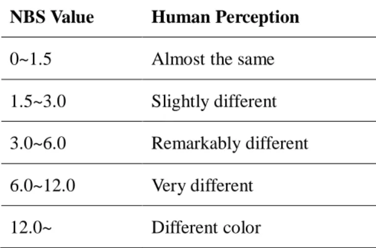
(28) Chapter 2. Color Space. H = arctan. S2 S1. ( 2.25). V = H3. ( 2.26). C = S12 + S 22. ( 2.27). To calculate the color difference in the HVC color space, we make use of National Bureau of Standards (NBS) color distance [28] instead of the Euclidean distance measure. The NBS color distance is similar to Godlove’s formula. For two colors (H1,V1,C1) and (H2,V2,C2), the color distance is:. dist = 1.2. ( 2C1C2 ) (1 − cos ( 2π∆H /100 ) ) + ( ∆C ) + ( 4∆V ) 2. 2. ( 2.28). where ∆H = H 1 − H 2 , ∆V = V1 − V2 , and ∆C = C1 − C2. It was found that in the HVC color space, the human color perception has close relation to the NBS color distance. The relation of human color perception and NBS distance is shown in Table 2.1. We know that if the NBS color distance of two colors below 1.5, human will regard the colors almost the same from the table. Table 2.1 The correspondence between the human color perception and the NBS distance. NBS Value. Human Perception. 0~1.5. Almost the same. 1.5~3.0. Slightly different. 3.0~6.0. Remarkably different. 6.0~12.0. Very different. 12.0~. Different color. 20.

(29) Chapter 3. Proposed System Model for Color Segmentation. Chapter 3. Proposed System Model for Color Segmentation 3.1 Overview In this chapter, several color segmentation approaches will be reviewed. Then the proposed method for color image segmentation will be followed. The whole system will be discussed detailed from section 3.1 to 3.4. And the principles and theories which are used in my proposed system will also be discussed. The overall algorithm will be shown in detail in the last section of this chapter. The color segmentation approaches are composed of monochrome segmentation approaches introduced in Chapter 1 and color spaces in Chapter 2. It can be shown in Fig.3.1. Most gray level image segmentation techniques can be extended to color images, such as histogram threshold, clustering, region growing, edge detection, fuzzy approaches and neural networks. Gray level segmentation methods can be combined with some other methods to obtain a final segmentation result [3]. However, one of the problems is how to employ the color information as a whole for each pixel. When the color is projected onto three components, the color information is so scattered that the color images becomes simply a multi-spectral image and the color information that humans can perceive is lost. Another problem is how to choose the color representation for segmentation. There are many color representation approaches and each one has its advantages and disadvantages. I will use all color spaces discussed in Chapter 2 to see which one has the better performance in my proposed algorithm, and which color space is suitable for region growing algorithm.. 21.

(30) Chapter 3. Proposed System Model for Color Segmentation. Fig. 3.1 Commonly used color image segmentation approaches [3].. 3.2 System Model The proposed color image segmentation algorithm is a region based approach. The advantage of region-based segmentation is that it considers both the color information and spatial details. The proposed algorithm is a series of region growing and merging process. It combines color information classification and region growing techniques [4]. Both techniques have their owned advantages and disadvantages for separating disjointed regions in color images. Some disadvantages of one technique can be overcome by the advantages of another to yield a much better segmentation results if we combine both techniques properly. The proposed algorithm starts with the region growing process, which groups pixels into homogeneous regions by combining the 3-D clustering and relaxation labeling techniques. And each resulting small region is then merged to its nearest region in terms of color similarity and spatial proximity. One problem with region growing is its inherent dependency on the selection of seed region, which can be avoided by using the relaxation labeling technique. It is an important part to solve how to choose appropriate seed points. After establishing the whole system, the different color space will be replaced by its origin RGB color space for clustering and region growing. The whole system flow chart is shown in Fig. 3.2. 22.

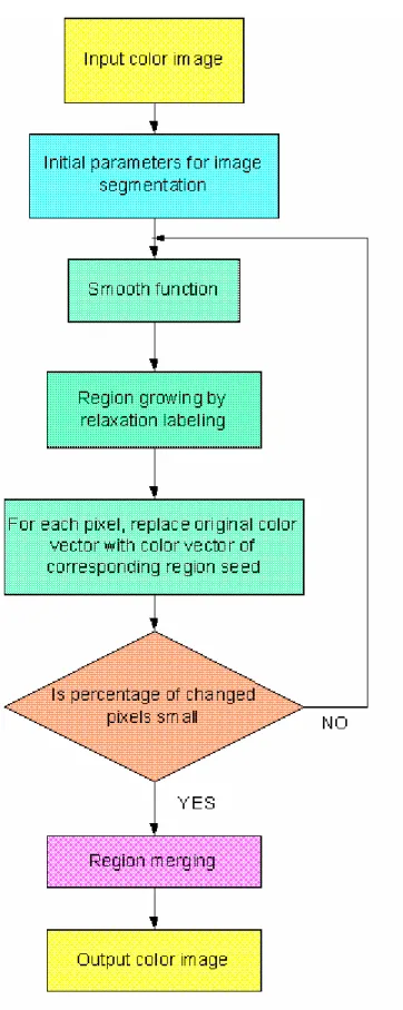
(31) Chapter 3. Proposed System Model for Color Segmentation. Fig. 3.2 Flowchart of the proposed algorithm.. 23.

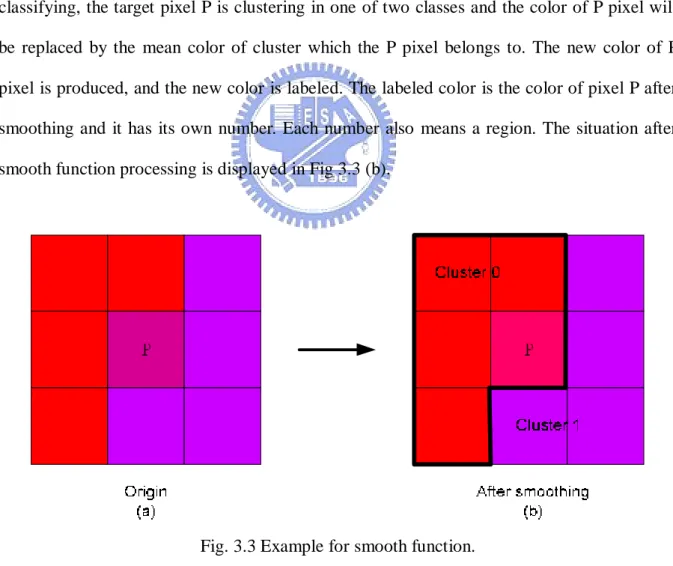
(32) Chapter 3. Proposed System Model for Color Segmentation. 3.3 Smooth and Cluster In this section, the smooth function shown in Fig. 3.2 will be addressed. The smooth function smooth a color image by 3-D clustering. The 3-D color clustering is to remove small objects or noise of a given input color image. The color clustering technique works as a pre-processing stage of a region-based approach. Similar to Mirmehdi and Petrou’s method [8], the proposed method uses a color clustering method for smoothing and relaxation labeling for region assignment of the pixels. In the proposed smooth function, K-means clustering method is used for smoothing color image. The K-means algorithm is similar to Forgy’s algorithm [29]. Besides the data, input to the algorithm consists of k, the number of clusters to be constructed. The K-means algorithm differs from Forgy’s algorithm in that the centroids of the clusters are recomputed as soon as a sample joins a cluster. The K-means algorithm are given below: K-means Algorithm: Step 1. Begin with k clusters, each consisting of one of the first k samples. For each of the remaining n-k samples, find the centroid that nearest to it. Put the sample in the cluster identified with this nearest centroid. After each sample is assigned, recompute the centroid of the altered cluster. Step 2. Go through the data a second time. For each sample, find the centroid that nearest to it. Put the sample in the cluster identified with this nearest centroid. (During this step, do not recompute any centroid.) The smooth function algorithm is shown below: SMOOTH (I,P,N) Algorithm: Step 1. Take the N x N neighborhood mask M of pixel P in a given input image I, where P is the center of mask M. Step 2. Using K-means clustering method to classify the pixels in M into two classes, Class 0 24.

(33) Chapter 3. Proposed System Model for Color Segmentation. (C0) and Class 1 (C1). Step 3. Computes the means C0 ’and C1’ for Class 0 and Class 1 respectively. And the pixel P is clustering belong to which cluster. Step 4. Let Cp' be the new label color of P which is the means of the cluster that the pixel P belongs to. It replaces the origin color of pixel P.. For example, if N=3, it is a 3 x 3 mask. The P is the target pixel in the mask center. It has nine pixels including P and each one has its own color as shown in Fig. 3.3 (a). Then it is going through the K-means algorithm to remove noise and to classify into two classes. After classifying, the target pixel P is clustering in one of two classes and the color of P pixel will be replaced by the mean color of cluster which the P pixel belongs to. The new color of P pixel is produced, and the new color is labeled. The labeled color is the color of pixel P after smoothing and it has its own number. Each number also means a region. The situation after smooth function processing is displayed in Fig 3.3 (b).. Fig. 3.3 Example for smooth function.. Every pixel in the color image will process this smooth function to remove noise and 25.

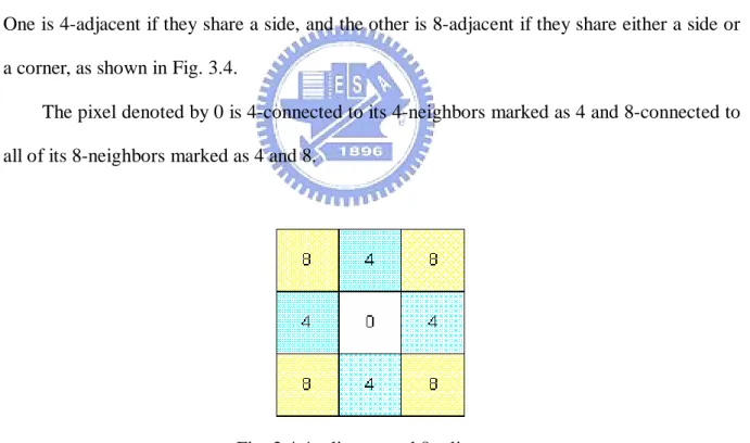
(34) Chapter 3. Proposed System Model for Color Segmentation. find label color information and seed points for region growing. This is an important pre-processing for region growing. The label color and the origin color may be the same or different. There are many ways for color clustering such as fuzzy c-means, principal component analysis [30], and etc.. 3.4 Labeling In order to identify which pixels belong to each specific region, we use labeling. By labeling, we can measure various properties for each individual region such as its size, shape, location, or color for image understanding. Before introducing labeling, the neighborhood which is adjacent to the pixel is defined. There are two ways to determine adjacent or not. One is 4-adjacent if they share a side, and the other is 8-adjacent if they share either a side or a corner, as shown in Fig. 3.4. The pixel denoted by 0 is 4-connected to its 4-neighbors marked as 4 and 8-connected to all of its 8-neighbors marked as 4 and 8.. Fig. 3.4 4-adjacent and 8-adjacent.. In this research, we use 8-adjacent way for labeling. Now we describe a labeling algorithm that replaces each pixel of image by a negative number representing the region to which the pixel belongs are not labeling yet. The algorithm uses a list to keep track of pixels that are unlabeled yet. This list also called a queue which has two operations: insert (m, n) 26.

(35) Chapter 3. Proposed System Model for Color Segmentation. which inserts the pixel (m, n) at the end of the list, and (m, n) ß remove( ) which removes the pixel from the front of the list and saves it for further use as the pixel (m, n). The algorithm begins by scanning the image from left to right, top to bottom. When an unlabeled pixel (x, y) is found, the algorithm will label all the pixels in the 8-connected region to which (x, y) belongs before it labels any pixels from other regions. We first obtain a new label L then label (x, y) as L and add (x, y) to an initially empty list of pixels whose neighbors are to be checked later. Next we remove the pixel (m, n) least recently placed in the list. We next label with L each unlabeled 4-neighbor of (s, t) that has the same character as (m, n) and insert each such 8-neighbor in the list such 8-neighbors belong to the same region as (m, n). We then repeat this process. If the list is not empty, we remove from the list the pixel (m, n) least recently placed in the list. We next label with L each unlabeled 8-neighbor of (m ,n) that has the same character as (m, n) and insert each 8-neighbor in the list. Whenever the list is empty, one entire region has been labeled, at which point this process is terminated and the process is repeated by scanning the image from left to right, top to bottom, looking for another unlabeled pixel. If such a pixel is found, we obtain a new label and restart the labeling process. The labeling algorithm can be expressed as follows: Region-Labeling Algorithm: Step 1. L ß -1 ( Initialize label) Step 2. Scan the image from left to right and top to bottom for all (x, y). If the pixel (x, y) conforms the requirement, then insert (x, y). While list is not empty do (m, n) ß remove() For each 8-neighbor (u, v) of (m, n) do If (u, v) is unlabeled and has same character with (x, y) Insert (u, v) end If end For end While L ß L-1 ( Get new label ) End scan 27.

(36) Chapter 3. Proposed System Model for Color Segmentation. 3.4.1 Relaxation Relaxation is an iterative process. For the specific problem of image thresholding, the thresholds for any given iteration are computed as a function of those in the same neighborhood at the previous iteration. The original scheme that will be followed is shown below [31]: Original Relaxation Method: Step 1. Create an initial guess at segmentation for the image. Provide an estimate of the confidence in that guess at each pixel. Step 2. For each pixel, modify the segmentation and the confidence estimate based on the pixels in the local region; the surrounding eight pixels will do. Step 3. Repeat step 2 until the segmentation is complete. This might be when no further changes are seen in successive steps.. The confidence estimates have the appearance of probabilities, although they may not be accurate in that regard. All that matters is that they are fairly accurate with respect to the other pixels, especially those in the local neighborhood. By applying an iterative scheme the local consistencies adjust to global consistencies in the whole image. There are many types of relaxation, some of them being used in statistical physics, while others are used in image understanding. To provide a better understanding of the idea, the discrete relaxation approach and probabilistic relaxation approach will be introduced.. 3.4.1.1 Discrete Relaxation Discrete relaxation assigns all existing labels to each object and iteratively removes all the labels which may not be assigned to an object violating the constraints. For example, consider the scene shown in Fig. 3.5 down below. Six objects are present in the image, 28.

(37) Chapter 3. Proposed System Model for Color Segmentation. including the background. Let the labels be background (B), window (W), table (T), drawer (D), and phone (P).. Fig. 3.5 Scene labeling example.. And the unary properties of object interpretations are: • A window is rectangular. • A table is rectangular. • A drawer is rectangular. The binary constraints are: • A window is located above a table. • A phone is above a table. • A drawer is inside a table. • Background is adjacent to the image border. Given these constraints, the labeling in Fig 3.6 is inconsistent.. 29.

(38) Chapter 3. Proposed System Model for Color Segmentation. Fig. 3.6 Inconsistent labeling. The possible relaxation sequence is shown below. At the beginning, all labels are assigned to each objects, and for each object all its labels are tested for consistency (Fig. 3.7(a)). Therefore, the label B can immediately be removed as inconsistent with objects 2, 3, 4, 5, and 6. Similarly, object 3 is not rectangular; therefore it violates the unary relation that must hold for T, W, D, etc. The final consistent labeling is given in figure 3.7(c).. (a) Where B (background), D (drawer), P (phone), T (table), and W (window). 30.

(39) Chapter 3. Proposed System Model for Color Segmentation. (b). (c) Fig 3.7 Discrete relaxation: (a) all labels assigned to each object; (b) locally inconsistent labels are removed; (c) final consistent labeling.. The discrete relaxation algorithm can be given below. Discrete Relaxation Algorithm [6]: Step 1. Assign all possible labels to each object, considering the unary constraints. Step 2. Repeat steps 3~5 until global consistency is achieved or is found to be impossible. Step 3. Choose one object to update its labels. Step 4. Modify labels of the chosen object by considering relations with other interacting objects. Step 5.If any object has no label, stop à a consistent labeling was not found.. 31.

(40) Chapter 3. Proposed System Model for Color Segmentation. 3.4.1.2 Probabilistic Relaxation Another kind of relaxation method is probabilistic relaxation. In discrete relaxation, it results in an unambiguous labeling in a majority of real situations. However it represents an oversimplified approach to image data understanding. It can not cope with incomplete or imprecise segmentation. Using semantics and knowledge, image understanding is supposed to solve segmentation problems which cannot be solved by bottom-up interpretation approaches. Probabilistic relaxation may overcome the segmentation problems of missing objects or extra regions in the scene, but it results in an ambiguous image interpretation which is often inconsistent. The probabilistic relaxation is similar to discrete relaxation. The object labeling depends on the object properties and on a measurement of compatibility of the potential object labels with the labeling directly interacting objects. All the image objects may be considered directly interacting and only adjacent objects are usually considered to interact directly. These two relaxation approaches differs in interpretation robustness. Discrete relaxation allows only one label to be assigned to each object in the final labeling. Effort is directed to achieving a consistent labeling all over the image. It always finds either a consistent labeling or detects the impossibility of assigning consistent labels to the image. But if the image is in imperfect segmentation, discrete relaxation fails to find a consistent interpretation even only a small number of local inconsistencies are detected. Probabilistic relaxation allows multiple labels to co-exist in objects. Labels are probabilistically weighted with a label confidence being assigned to each object label. It always gives an interpretation result together with a measure of confidence in the interpretation. Even if the result may be locally inconsistent, it often gives a better image interpretation than a consistent and possibly very unlikely interpretation resulting from a discrete labeling. Note that discrete relaxation may be considered a special case of probabilistic labeling with one label probability always being 1 and all the others being 0 for 32.

(41) Chapter 3. Proposed System Model for Color Segmentation. each object.. 3.4.2 Relaxation Labeling As mentioned before, each pixel of the image will pass through the smooth function to smooth the noise and find the particular seed points. If a pixel P is going to input to smooth.  org. function like figure 3.2, we first record its original color as vector C p . It means the pixel P’s color information, for example, Rorgp, Gorgp, and Borgp in RGB color space. In each color space, it records corresponded color information. After it passing through the smooth function,  lab. the pixel P will has its new color. It is expressed with vector C p . Just like the meaning of  org C p , it records its R, G and B color information in RGB color space. Then we define an attribute d[] as the Euclidean distance which is the difference between the original color information and the label color information of the pixel. So d[p] means the difference between origin color and label color after smooth function of pixel P. It can be computed by:  org  lab d [ p ] = D (C p , C p ) lab 2 org lab 2 org lab 2 = ( R org p − R p ) + (G p − G p ) + ( B p − B p ). ( 3.1). Where the last equation is perform in original color space RGB. We also call it a label-error estimate. To employ the pixel grouping process for region growing by relaxation labeling technique, we first initialize parameters as shown in Fig. 3.2. After initializing the system, the process of relaxation labeling is carried out for each pixel. We define the relaxation labeling operator over each pixel as:.   l a b  C laq b   C p    r n[ p ]  r n[ q ] =   la b  o r g  d [q ]      D ( C p , C q.     ) . 33. ( 3.2).

(42) Chapter 3. Proposed System Model for Color Segmentation. if d [ q ] > d [ p ] + w p , q. ( 3.3). Where p is the main pixel in the center of the mask and q is a neighborhood pixel of pixel p. And rn[ ] is the region number of the pixel, for instance, rn[p] is the region number of pixel p and so on. D(a, b) is the Euclidean distance between two color vector a and b. The weight wp,q means the constraint to avoid merging the pixels p and q. It also indicates if the  org  org pixel q and p belong to the same region. Here, wp,q are set to be D(C p , C q ) . If the condition is satisfied, the information associated to q is changed. The label color of pixel q is been update to label color of pixel p, and the region number of q ( rn[q] ) is changed to the same as the region number of p ( rn[p] ). The label-error estimate of pixel q ( d[q] ) is replaced  lab  org by D(C p , C q ) which is the new label-error estimate of pixel q. The process of relaxation. labeling a neighboring pair pixel (p, q) consists of testing whether we can improve the label-error of q by going through the relaxation labeling operator of p and, if it conforms the condition, updating the data as shown in equation. As shown in Fig. 3.8, a relaxation step may group the pixels p and q together and decrease the value of the label-error estimate d[q]..  lab Cp.  lab Cq. rn[p].  lab  org D (C p , C q ).  org Cp. w p ,q.  org Cq. Fig 3.8 A relaxation labeling step. If d [ q ] > d [ p ] + w p , q , not only the value of d[q] is decreased by replacing the label color of q with that of p but also set the pixel q with the same region label number as pixel p. 34.

(43) Chapter 3. Proposed System Model for Color Segmentation. Pixel p is so called the seed point, and this action is called relaxation labeling. After relaxation labeling operator, the region number and the label color of pixel q is as same as pixel p. Every pixel in the image will do the relaxation labeling operator if the relaxation pixel is determined as a seed point after passing through the smooth function. Note that the value of label-error d[ ] may achieve its lower bound after a few iterations.. 3.5 Region Merging When the image has already been segmented into regions, the regions must satisfy the following conditions：. H ( Ri ) = TRUE. i=1, 2, …, S. H ( Ri ∪ R j ) = FALSE. i≠j , Ri adjacent to Rj. ( 3.4). where S is the total number of regions in an image and H(Ri) is a homogeneity evaluation of the region Ri. Resulting regions of the segmented image must be both homogeneous and maximal. Where ‘maximal’ means that the homogeneity would not be same after region merging with any adjacent region. The general region merging algorithm is given below: Region Merging Algorithm Step 1. Define some starting method like relaxation labeling to segment the image into many small regions satisfying condition ex: Eq. 3.3. Step 2. Define a criterion such as Eq. 3.5 for merging two adjacent regions. Step 3. Merge all adjacent regions satisfying the merging criterion. If no more regions can be merged while maintaining condition Eq. 3.5 is satisfied, then stop. Otherwise go to Step 2.. Among the regions obtained in the previous section, only parts of them are really characteristic, so the other regions need to be merged into them. Here we use specific method 35.

(44) Chapter 3. Proposed System Model for Color Segmentation. differs from the general region merging algorithm in the criterion for merging. The image has already been segmented to several small regions from relaxation labeling shown in last section. We consider that the regions which have smaller values of the spatial color diversity rates. Not only consider the color between the regions but also the space position of each region to determine whether it merges or not. We define the spatial color diversity rate of a region R as:. color _ diveristy ( R ) =. ∑.   D (C p , C q ). ∑. p∈R q∈neighbors ( p ). ∑I. ( 3.5). p∈ R. . . Where neighbors(p) means the set of pixels which are spatially adjoining p and C p , C q are the color vectors of pixels p and q. The denominator of color_diversity rate is the number of pixels which are in the same region R. The numerator of color_diversity rate represents that every pixel which is neighboring upon the pixels in the same region R to calculate each value of color difference defined in Eq. 3.1 and then sum them total. The definition of Eq. 3.5 has considered both color information and spatial information for region merging. It is specifically and predominantly than other region merging algorithms.. 3.6 The Proposed Algorithm The proposed algorithm will be shown in detail including region growing by relaxation labeling and region merging in sequential below. Proposed Algorithm: Step 1. Input a color image and initialize all the parameters like rn[], weighting, ND, and etc. Then the region growing process is beginning. Step 2. If it is the first time of the process, for each pixel p in the image, the SMOOTH function will be executed to compute label color and d[p]. Else go to Step 4. 36.

(45) Chapter 3. Proposed System Model for Color Segmentation. Step 3. For each pixel p, replace original color vector with label color vector if they are different. If the percentage of modified pixels is small, the pixels with the same region number will be grouped together to form initial regions as the preliminary for region merging. Then the region growing process is finished and region merging process is begun. Go to Step 10. Else when the percentage of modified pixels is not small, go to Step 2. Step 4. For each pixel p, the SMOOTH function will be executed to compute label color and add the pixel p to a pixel set Q if d[p] is decreased. If the pixel set Q is empty. Go to Step 3. Step 5. From the pixel set Q, extract a pixel p which has the minimum value d[]. If the pixel p has already assigned a region, it will go on the next step. Else, go to Step 8. Step 6. Find the pixel q which is the nearest neighbor of the pixel p and conform the condition d[p]>d[q]+wp,q. If we do find the pixel q, the next step will be started. Else, go to Step 9. Step 7. If the nearest neighbor pixel q has already been assigned a region. Relax the pair (q,p) by relaxation labeling by Eq.(3.2) and Eq. (3.3) then go to Step 9. Else, go to Step 8. Step 8. Assign pixel p a new region number from the number of RN and increase RN on one then go to the next step. Step 9. For each neighbor pixel q of p, relax pair (p, q) according to equation and add q to the pixel set Q if q is not in Q and d[q] is decreased, and also remove p from Q. Then go to Step 5. Step 10. The region merging process is started. For each region segmented by relaxation labeling Ri, i=1, …, NR, Eq.(3.5) will be used to compute its owned spatial color diversity rate. Step 11. Construct a region queue RQ consisting of all regions in the image by sorting regions according to size of regions. Set threshold t to be an average value of spatial color 37.

(46) Chapter 3. Proposed System Model for Color Segmentation. diversity rate of all regions in the RQ. Step 12. If the region number from region growing NR is equal to the desired region number ND, the region merging process is finished. The final result will be output. Else go to the next step. Step 13. Extract a region Ri with the minimum size from RQ. If the color diversity of region Ri is greater than the threshold t, the region which is less representative spatially will be merged into the region which is nearest to it in colorimetrical. Else, each pixel of the region will be merged into the region which is the nearest to it in colorimetrical and surrounds it spatially. Step 14. A region was been merged so we minus the NR on one. Then go to Step 12.. The proposed algorithm is combined with the region growing process and region merging process shown in Fig.3.9 and Fig 3.10. After region growing by relaxation labeling process, the image will be segmented to many small regions. But most of them are not important or with less information. In order to eliminate these tiny regions, we are going to do region merging to reduce these regions and preserve the regions which are important and have most information of the image. The whole procedure will be completed when the region merging process is accomplished. The image after processing the algorithm will maintain the most color information of the color of the image. So we can use less character to implement the image, it can let the image easy to express and easy to recognize as image understanding. It also can save the transmission cost. For example, if we set the desired region number as 32, than the final image just has 32 colors to implement the image no matter how many color represent the image from the beginning. Basic on this algorithm, the color image with different color spaces will input to the algorithm seeing which color space has the best performance in this algorithm.. 38.

(47) Chapter 3. Proposed System Model for Color Segmentation. Fig 3.9 Flowchart of proposed region growing by relaxation labeling algorithm. 39.

(48) Chapter 3. Proposed System Model for Color Segmentation. Fig. 3.10 Flowchart of region merging algorithm [3]. 40.

(49) Chapter 5. Conclusion and Future Work. Chapter 4. Experimental Results 4.1 Experiment Results The experimental results of the proposed algorithm with different color space will be shown in this section. It will illustrate the effectiveness of the proposed segmentation algorithm and color space in color images. The experimental results presented are obtained by using an Intel Pentium 4 2.4 GHz PC, and the input images size are 512 x 512 BMP form files. All the input images were digitized to 24 bits per pixel and the final desired regions are set to be 64. The proposed algorithm has been coding in Visual C++ Studio.Net.. (a). (b). (c). (d). Fig 4.1 Origin input color image (a) fruit (b) plane (c) pool (d) baboon.. 41.

(50) Chapter 5. Conclusion and Future Work. (a). (b). (c). (d). (e). (f). Fig 4.2 Output resulting fruit image. (a) RGB (b) YIQ (c) I1I2I3 RGB) (e) HSI (f) HVC. (d) nRGB (normalized. (a). (b). (c). (d). (e). (f). Fig 4.3 Output resulting plane image. (a) RGB (b) YIQ (c) I1I2I3 RGB). (e) HSI 42. (f) HVC. (d) nRGB (normalized.

(51) Chapter 5. Conclusion and Future Work. (a). (b). (c). (d). (e). (f). Fig 4.4 Output resulting pool image. (a) RGB (b) YIQ (c) I1I2I3 RGB) (e) HSI (f) HVC. (d) nRGB (normalized. (a). (b). (c). (d). (e). (f). Fig 4.5 Output resulting baboon image. (a) RGB (b) YIQ (c) I1I2I3 (d) nRGB (normalized RGB). (e) HSI 43. (f) HVC.