在無線網路中用馬可夫決策開發多個使用者之間的多樣性以達到有彈性的傳輸

國 立 交 通 大 學

電信工程學系

碩 士 論 文

在無線網路中用馬可夫決策開發多個使用者之

間的多樣性以達到有彈性的傳輸

Multi-user Diversity for Flexible

Communications in Wireless Networks by MDP

研究生：林柔嫚

指導教授：廖維國 博士

在無線網路中用馬可夫決策開發多個使

用者之間的多樣性以達到有彈性的傳輸

Multi-user Diversity for Flexible

Communications in Wireless Networks by MDP

研 究 生︰ 林柔嫚

Student: Jou-Man Lin

指導教授︰ 廖維國 博士

Advisor: Dr. Wei-Kuo Liao

國 立 交 通 大 學

電信工程學系碩士班

碩士論文

A Thesis Submitted to

the Department of Communication Engineering

College of Electrical and Computer Engineering

National Chiao Tung University

in Partial Fulfillment of the Requirements

for the Degree of Master of Science

In

Communication Engineering

Sep 2006

Hsinchu, Taiwan, Republic of China

在無線網路中,基於馬可夫決策,如何開

發多個使用者之間的多樣性

研 究 生︰ 林柔嫚

指導教授︰ 廖維國 博士

國立交通大學電信工程學系碩士班

中文摘要

多個使用者之間的多樣性(Multi-user diversity)，所指的是在一個無線網 路中，因為多個用戶間的頻道狀態不同，造成的多種變化。這種多樣性可經由安 排用戶的傳輸先後次序來增進效能，安排的方式是採用讓擁有較適合傳輸的用戶 來進行傳輸。利用這樣的方法使得系統的傳輸能力隨著用戶數目增加而提高。在 這篇論文當中，我們考慮利用分散式的方法增進多個使用者之間的多樣性。在現 今的多媒體通訊下，封包有重要性的差別，例如語音傳輸的封包有時效性的限 制，損失這樣的封包對於系統的品質可能造成極大的影響，其重要性就比可容忍 長時間延遲的資料封包來的重要。所以我們必須考慮封包遺失對於系統所造成的 影響以及如何增進多個使用者之間的多樣性。為了處理這樣的問題，廖教授與葉 學長提出利用 minimax-Markov-Decision 的方式來處理固定長度的封包，但是在 他們的研究中只採用了 ARQ 的錯誤控制方法。然而，我們要討論的問題是希望能 夠處理長度不固定的封包，所以更為困難。廖教授以及黃學長討論以混合 ARQ 跟 FEC 的錯誤控制方式來處理這樣的問題，我們想要更進一步的研究如何增進多個 使用者之間的多樣性。我們將問題用 Markov Decision Process 來描述，並且我 們針對最糟糕的情況來加以討論。我們觀察因為遺失封包所導致的損失，而且與 另外的兩種方法比較，經由模擬結果可得知，我們所採用的方法造成的損失，的 確比其他方法還要少。

Multi-user Diversity for Flexible

Communications in Wireless Networks by

MDP

tStudent: Jou-Man Lin Advisor: Dr. Wei-Kuo Liao

Department of Communication Engineering

National Chiao Tung University

Abstract

Multi-user diversity refers to a type of diversity across different users in a fading environment. This diversity can be exploited by scheduling transmission so that users transmit when their channel conditions are favorable. Using such an approach leads to a system capacity that increases with the number of users. In this thesis, we consider exploiting multi-user diversity in a centralized way for the flexible communication over wireless channels. Because the importance of packets is different in multi-media communication, loss of the important packet will probably degrade the system performance hugely. We need to consider both the effect of packet loss and the multi-user diversity issue. To handle such a problem, Liao and Yeh propose a minimax-Markov-decision approach which considers fixed-length packet and automatic-repeat-request (ARQ). However, our problem is more difficult due to the various lengths of packets. Liao and Huang consider a hybrid ARQ model to deal with this problem, and we extend their research to multi-user diversity part. We model our problem as a Markov Decision Process and we consider the worst case in our simulation. We evaluate the performance in terms of the cost induced by the packet loss, and observe improvements against traditional fair queuing algorithm and a greedy method which only give transmission chance to the mobile with the best channel condition.

誌謝

首先，感謝指導教授廖維國老師，從大四的專題實驗，到研究所的兩年 時光，老師都給予我許多的指導 ; 也感謝清華大學的金仲達老師，以及交通大 學的張仲儒老師，能夠在百忙之中抽空前來參加口試，並給予我論文上的指導與 建議。 終於完成一篇屬於自己的論文，我內心的雀躍真是筆墨無法形容的 ; 回顧這兩年的研究所生涯， 不論是期末考的挑燈苦讀、還是跟實驗室的大家一 起歡唱 KTV …，都是我的美好回憶。此時此刻，我的內心真可說是百感交集， 一方面正期待完成碩士學業的未來生活，另一方面也對即將離開待了六年的交通 大學感到不捨。 尤其是充滿歡樂的 812b 實驗室，大家給予我這溫暖的友情， 是我一輩子也不會忘記的 ; 學長 TACO 還有小智在我研究遇到瓶頸時，主動提 供我相關的資訊，適時點醒我心中的盲點 ; 毛毛、陳佳甫、林裕翔，陳為凡是 我研究所同甘共苦的好夥伴，一起討論課業，一起打屁嬉鬧 。 從小到大，媽咪跟姐姐在我遭遇挫折的時候，總是給我鼓勵，教導我相 信自己，相信一定能突破困難，使我學會樂觀的看待生活中的不順遂 。 最後，我要感謝子逸，在這六年的日子裡，一路陪伴着我，給我依靠， 不論開心或難過，都想跟你分享。 謝謝大家。 2006 年 9 月

Contents

Chinese Abstract………...……2 English Abstract……….. 3 Acknowledgement………....4 Contents……….………5 List of Tables……….………6 List of Figures……….………. 6 Chapter 1: Introduction………….………. 8 Chapter 2: Background……….……….... 10 2.1 Multi-user Diversity……….………….…….…10

2.2 Start-time Fair Queuing………..11

2.3 MAC Frame Structure……….…….…………..12

2.4 Reed-Solomon Code……….……….12

2.5 Markov Decision Process……….….…….13

I. The Policy-Iteration Method..……….…..………15

II. The Value Determination Operation……..………..……….16

III. The Policy improvement Routine...………….…..………..…….17

IV. A Proof of the Properties of the Policy-Iteration Method…...……..…20

Chapter 3: System Specification…………...…….………...22

3.1 Mobile Model.……….……..………...…..23

3.2 Channel Model………….…..………25

3.3 Base-Station Model…….…..…………..……..……….26

Chapter 4: Problem Formulation Based on MDP ….….……….…….……….….28

4.1 State Definition………...………...30

4.2 Action Space………...30

4.3 State transition probability……….…………...………...…...30

4.4 Packet Cost………...…………...…32

4.5 State Transition Probability…...………..………...…32

4.6 Policy Iteration………..……….33

4.7 Worst Inter-Polling Time………....33

Chapter 5: Simulator Design…….………35

MDP Program and Simulator Setting……….……..35

Chapter 6: Simulator Results..………...………..….39

6.1 Short term Average Cost……….…….………...39

6.2 Long term Average Cost………..………...42

6.3 Packet Loss Performance………...45

Reference……….52

List of Tables

Number Page 1.1 A class of adaptive RS code………...21

4.1 Actions………....29

5.1 Packet error rate in different situation………36

List of Figures

Number Page 2.1 MAC frame structure……….11

2.2 The iteration cycle………..18

3.1 Framework for a wireless link………....22

3.2 Gilbert model………..24

4.1 State Encoding………28

4.2 Transition diagram………..30

4.3 Worst case………...33

5.1 UML state-chart for base-station...……….35

5.2 UML state-chart for mobiles………..………38

6.1 Simulation Results of Unchanged Cost (fair queue and cost compare).39 6.2 Simulation Results of Unchanged Cost (cost compare and channel compare)………...39

6.3 Simulation Results of changed Cost Case 2(cost compare and channel compare)………...39

6.4 Simulation Results of changed Cost Case 3(cost compare and channel compare)…...………41

6.5 Simulation Results of changed Cost Case 2(fair queue and cost compare)………...41

6.6 Simulation Results of changed Cost Case 3(fair queue and cost compare)………...42

6.7 Simulation Results of Unchanged Cost (Long Term)………43

6.8 Simulation Results of Changed Cost Case 3(Long Term)………..43

6.9 Packet Loss of Cost Unchanged……….45

6.10 Packet Loss of Cost Change Case (3)………..46

6.12 Packet Loss of Cost Unchanged and Window =1………..……..47 6.13 Packet Loss of Cost Unchanged and Window =2………..…………..47 6.14 Packet Loss of Cost Unchanged and Window =max=3…………...…48 6.15 Packet Loss of Cost Change Case (3) and Window =0…………..…..49 6.16 Packet Loss of Cost Change Case (3) and Window =1………..……..49 6.17 Packet Loss of Cost Change Case (3) and Window =2…………..…..50 6.18 Packet Loss of Cost Change Case (3) and Window =max=3………...50

Chapter 1

Introduction

Wireless channels suffer from fading effects, due to user’s mobility and the interference from other users. Because of this time-varying situation, the channel condition changes from time to time. When there are many users in the system, different users will experience peaks in their channel quality at different time. The effect has been shown to exploit by scheduling the user with favorable channel conditions.

When combing with the packet loss effect with the channel condition, the situation become complicated. For example, in MPEG, packet is with different significance to the quality and a loss of a packet with higher importance, e.g., the I-frame packet, will bear the higher chance to let user to experience the quality degradation. Therefore tradeoff arises if two connections have the conflicting condition -- one connection has the worse channel condition, i.e., less chance to have successful transmission, but more important packet waiting to be sent. As a result, chances to impact the quality are hard to be compared between these two connections. For this reason, it may not be the best strategy to always grant the transmission to the user with the best channel condition.

To this end, The flexible communication scheme based on TDMA is originally proposed by Liao and Yeh[9], where they define the flexible concept by treating the packets to be correctly transmitted as jobs and wireless bandwidth as resources. Through their research, they consider the fixed-length packet and automatic repeat request (ARQ) and use minimax-Markov-decision approach to develop their transmission strategy. Besides, a way to exploiting the multi-user diversity gain for downlink transmission is also proposed in their research.

The problem becomes more difficult to handle if the packets with various lengths are allowed to be transmitted over the wireless channel. In multimedia traffic, packets are compressed with different compress ratio and thus come with different length. Besides, to resist the transmission error, redundancy code can be selectively equipped with the packet and thus the variation of packet length can be further inflated. To cope with such a problem, Liao and Huang work [10] on hybrid ARQ, ARQ plus forward error correction, for flexible communication are proposed. However, they did not

discuss the topic on exploiting the multi-user diversity gain.

Our research is considered as the extension of Huang’s work on Hybrid ARQ. That is, based on his work, we consider multi-user diversity issue in uplink transmission. The problem under our study is formulated as to minimize the cost induced by packet loss. We solve this problem with a Markov Decision Process. Based on the MDP approach, we find the optimal solution via the policy iteration and the technique so-called “one-step policy improvement.” In downlink transmission, all queued information is in the base-station. Therefore, downlink transmission is a special case of uplink transmission, when the delay of queued information is zero.

The rest of the thesis is organized as follows. In chapter 2 we introduce the background knowledge of our study. The system framework is presented in chapter 3. And the formulation of Markov Decision Process is described in chapter 4. The design in our simulator is illustrated with simulator graphs in chapter 5. Simulation results are reported in chapter 6, followed by conclusion in chapter 7.

Chapter 2

Background knowledge

In this chapter we will introduce the basic concept of RS code and MAC frame structure [1], multi-user diversity issue [2], start-time fair queuing [10], Markov Decision Process [3] with rewards and give formal definition to reward, alternative, expected cost value, and policy. We also introduce the Policy iteration method, which will lead us to find the optimal policy for the system.

2.1 Multi-user Diversity

A fundamental trait of wireless channels is that they exhibit fading effects, due in part to mobility and other user interference. As a result of this time-variation, a user’s channel suffers periods of severe decay, but also periods when the channel gain is stronger than average. When many users are present, different users will experience peaks in their channel quality at different times. This effect has been called multi-user diversity. It can be exploited by scheduling transmissions when a user has favorable channel conditions. The more users that are present, the more likely it is that one user has a very good channel at any time; hence, the total throughput of such a system tends to increase with the number of users. Given the channel gain of each user, it is shown that capacity is maximized by allowing only the user with the best channel to transmit at any time.

2.2 Start-time Fair Queuing

In our communication system, mobiles decide the code rate of packets, and base-station doesn’t know the length of packets unless they arrive. Because a packet length is unavailable a prior, we use start-time fair queuing algorithm in our thesis.

In Start-time Fair Queuing (SFQ) algorithm, two tags, a start tag and a finish tag, are associated with each packet. However, unlike WFQ and SCFQ, packets are scheduled in the increasing order of the start tags of the packets. Furthermore, v t is ( ) defined as the start tag of the packet in service at time t. The complete algorithm is defined as follows:

1. On arrival, a packet p_fj is stamped with start tag S p( _fj), computed as:

1

( _fj) max{ ( ( _fj)), ( _fj )} 1,

S p = v A p F p − j≥ (2.1) where F p( _fj), the finish tag of packet p_fj, is defined as:

( ) ( ) 1, j f j j f f f l F p S p j r = + ≥ (2.2)

where F p( 0_f)=0 and r_f is the weight of flow f

2. Initially, the server virtual time is 0. During a busy period, the server virtual time at time t , ( )v t , is defined to be equal to the start tag of the packet in service at

time t . At the end of a busy period, ( )v t is set to the maximum of finish tag

assigned to any packets that have been serviced by time t .

3. Packets are serviced in increasing order of the start tags; ties are broken arbitrarily.

2.3 MAC Frame Structures

Header User Data CRC

Header Segment Segment Segment

BCH coding redundant bits for

the header

RS coding redundant bits for the data and CRC

Figure 2.1 MAC frame structure.

As [1], for the MAC frame header, we adopt Bose–Chaudhuri–Hocquenghem (BCH) codes. The user data plus CRC is divided into segments, and each segment is encoded by an RS code.

2.4 Reed-Solomon (RS) Codes

For the error control of user data, we adopt (N,K,q) RS codes over GF(q) ,

in which the codeword size N and the number of information symbols K( N< ) .

A q -ary symbol is mapped tobbits, so q=2b. RS codes are known to have the maximum error -correction capability for given redundancy, i.e., a maximum distance separable (MDS) code.

For an (N,K) MDS code, the minimum distance dmin is determined as

1

min = N −K +

d , where the error correction capability t=(d_min −1)/2=(N −k)/2,

i.e., any combination of t symbol errors out of N symbols can be corrected. The

code rate r is defined as c rc =K/N. One can easily see that the more parity

symbols (i.e., larger N − ), the better error-correction capability. RS codes are K

also known to be efficient for handling burst errors. For example, with (N,K,2b)

RS code with the error correction capability t , as many as b t⋅ bit errors can be

corrected in the best case when all of b bits in each of tb-bit symbols are erroneous

one bit in each of tb-bit symbols is erroneous (i.e., non-burst errors).

Originally, the codeword size of (N,K,q) RS code is determined to beq−1.

However, a shorter codeword can be obtained via code shortening. For example,

given an (N,K,q) code, K− information symbols are appended bys s zero

symbols. These K symbols are then encoded to make an N symbol-long codeword.

By deletingsall zero symbols from the codeword, we can obtain(N−s,K −s)code.

For decoding this shortened code, the original(N,K)decoder can still be used by

appending zero symbols between K− information symbols and s N − parity K

symbols. Shortened RS codes are also MDS codes. Code shortening is useful

especially for transmitting information with less thanK symbols.

2.5

Markov Decision Process

Suppose that an N-state Markov process earns rij dollars when it makes a

transition from state i to state j. We call rij the “reward” associated with the transition

from i to j. the set of rewards for the process may be described by a reward matrix R

with elements rij. The rewards need not be in dollars, they could be voltage levels,

units of production, or any other physical quantity relevant to the problem.

The Markov process now generates a sequence of rewards as it makes transitions from state to state. The reward is thus a random variable with a probability distribution governed by the probabilistic relations of the Markov process.

One question we might ask concerning is: What will be the player’s expected winning in the next n transitions if the process is now in state i? To answer this question, let us define vi(n) as the expected total rewards in the next n transitions if the

system is now in state i.

Some reflection on this definition allows us to write the recurrent relation,

1 ( ) [ ( 1)] 1, 2, , 1, 2, 3, , N i ij ij j j v n p r v n i N n = =

∑

+ − = " = " (2.3)

If the system makes a transition from i to j, it will earn the reward rij plus the

amount it expects to earn if it starts in state j with one move fewer remaining. As

shown in Eq. 2.3, these rewards from a transition to j must be weighted by the

probability of such a transition, pij, to obtain the total expected rewards.

Notice that Eq. 2.3 may be written in the form

1 1 ( ) ( 1) 1, 2, , 1, 2, 3, , N N i ij ij ij j j j v n p r p v n i N n = = =

∑

+

∑

− = " = " (2.4)

so that if a quantity q is defined by i

1 1, 2, , . N i ij ij j q p r i N = =

∑

= " (2.5)

Eq. 2.3 takes the form

1 ( ) ( 1) 1, 2, , 1, 2, 3, . N i i ij j j v n q P v n i N n = = +

∑

− = " = " (2.6)

The quantity qi may be interpreted as the reward to be expected in the next

transition out of state i; it will be called the expected immediate reward for state i.

Rewriting Eq. (2.3) as Eq. (2.6) shows us that it is not necessary to specify both a P matrix and an R matrix in order to determine the expected earnings of the system. All

that is needed is a P matrix and a q column vector with N components qi. The

reduction in data storage is significant when large problems are to be solved on a digital computer. In vector form, Eq. (2.6) may be written as

( )n = + (n−1) n=1, 2, 3, ,

v q Pv " (2.7)

where v(n) is a column vector with N components vi(n), called the total-value

vector.

Consider a completely ergodic N-state Markov process described by a

transition-probability matrix P and a reward matrix R. Suppose that the process is allowed to make transitions for a very, very long time and that we are interested in the earnings of the process. The total expected earnings depend upon the total number of transitions that the system undergoes, so that this quantity grows without limit as the number of transitions increases. A more useful quantity is the average warnings of the process per unit time. This quantity is meaningful if the process is allowed to make many transitions; it was called the gain of the process.

Since the system is completely ergodic, the limiting state probabilities πi are

independent of the starting state, and the gain g of the system is

1 , N i i i g

π

q = =

∑

(2.8) where qi is the expected immediate return state i defined by Eq. (2.5).

I. The policy-Iteration Method

The policy-iteration method that will be described will find the optimal policy in a small number of iterations. It is composed of two parts, the value-determination operation and the policy-improvement routine. We shall first discuss the value-determination operation.

II. The Value-Determination Operation

Suppose that we are operating the system under a given policy so that we have specified a given Markov process with rewards. If this process were to be allowed to

operate for n stages or transitions, we could define vi(n) as the total expected reward

that the system will earn in n moves if it starts from state i under the given policy.

The quantity vi(n) must obey the recurrence relation Eq. (2.7). There is no need

for a superscript k to appear in this equation because the establishment of a policy has

defined the probability and reward matrices that describe the system.

For completely ergodic Markov processes vi(n) had the asymptotic form:

v ni( )=ng+vi i = 1, 2, ... , N for large n. (2.9)

1 1 1 1 1 [( 1) ] i = 1, 2, ... , N ( 1)

Since 1, these equations become

1, 2,..., N i i ij j j N N i i ij ij j j j N ij j N i i ij j j ng v q p n g v ng v q n g p p v p g v q p v i N = = = = = + = + − + + = + − + = + = + =

∑

∑

∑

∑

∑

(2.10)

We have now obtained a set of N linear simultaneous equations that relate the

quantities vi and g to the probability and reward structure of the process. However,

account of unknowns reveals N vi and 1 g to be determined, a total of (N+1)

unknowns. The nature of this difficulty may be understood if we examine the result of adding a constant a to all vi in Eqs. (2.9). These equations become

1 ( ), N i i ij j j g v a q p v a = + + = +

∑

+ or 1 . N i i ij j j g v q p v = + = +

∑

The original equations have been obtained once more, so that the absolute value of the vi cannot be determined by the equations. However, if we set one of the vi equal

to zero, perhaps vN, then only N unknowns are present, and the Eq. (2.8) may be

solved for g and the remaining vi. Notice that the vi so obtained will not be those

defined by Eq. (2.7) but will differ from them by a constant amount. The vi produced

by the solution of Eq. (2.8) with vN = 0 will be sufficient for our purposes; they will be

called the relative values of the policy.

We have now shown that for a given policy we can find the gain and relative

values of that policy by solving the N linear simultaneous equations with vN = 0. We

shall now show how the relative values may be used to find a policy that has higher gan than the original policy.

III. The Policy-Improvement Routine

We found that if we had a optimal policy up to stage n, we could find the best alternative in the ith state at stage n+1 by maximizing

1 ( ), N k k i ij j j q p v n = +

∑

(2.11) over all alternatives in the ith state. For large n, we could substitute Eq. (2.9) to obtain

1 ( ), N k k i ij j j q p ng v = +

∑

+ (2.12) as the test quantity to be maximized in each state. Since

1 1, N k ij j p = =

∑

the contribution of ng and any additive constant in the vj becomes a test-quantity

component that is independent of k. Thus, when we are making our decision in state i,

we can maximize 1 , N k k i ij j j q p v = +

∑

(2.13)

with respect to the alternatives in the ith state. Furthermore, we can use the relative

values (as given by Eqs. (2.9)) for the policy that was used up to stage n.

The policy-improvement routine may be summarized as follows: For each state i,

find the alternatives k that maximizes the test quantity

1 , N k k i ij j j q p v = +

∑

using the relative values determined under the old policy. The alternative k now

becomes di, the decision in the ith state. A new policy has been determined when this

procedure has been performed for every state.

We have now, by somewhat heuristic means, described a method for finding a policy that is an improvement over our original policy. We shall soon prove that the new policy will have a higher gain that the old policy. First, however, we shall show how the value-determination operation and the policy-improvement routine are combined in an iteration cycle whose goal is the discovery of the policy that has highest gain among all possible policies.

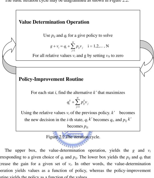
The basic iteration cycle may be diagrammed as shown in Figure 2.2.

Figure 2.2 The iteration cycle.

The upper box, the value-determination operation, yields the g and vi

corresponding to a given choice of qi and pij. The lower box yields the pij and qi that

increase the gain for a given set of vi. In other words, the value-determination

operation yields values as a function of policy, whereas the policy-improvement routine yields the policy as a function of the values.

We may enter the iteration cycle in either box. If the value-determination operation is chosen as the entrance point, an initial policy must be selected. If the cycle is to start in the policy-improvement routine, then a starting set of values is necessary. If there is no a priori reason for selecting a particular initial policy or for choosing a certain starting set of values, then it is often convenient to start the process

in the policy-improvement routine with all vi = 0. In this case, the

policy-improvement routine will select a policy as follows:

For each i, it will find the alternative k’ that maximizes qik and then set di = k’.

Value Determination Operation

Use pij and qi for a give policy to solve

For all relative values vi and g by setting vN to zero

1 i = 1,2,... , N N i i ij j j g v q p v = + = +

∑

Policy-Improvement Routine

For each stat i, find the alternative k’ that maximizes

1 N k k i ij j j q p v = +

∑

Using the relative values vi of the previous policy. k’ becomes

the new decision in the i-th state, qi k’ becomes qi, and pij k’

This starting procedure will consequently cause the policy-improvement routine to select as an initial policy the one that maximizes the expected immediate reward in each state. The iteration will then proceed to the value-determination operation with this policy, and the iteration cycle will begin. The selection of an initial policy that maximizes expected immediate reward is quite satisfactory in the majority of cases.

At this point it would be wise to say a few words about how to stop the iteration cycle once it has done its job. The rule is quite simple: The final robust policy has been reached (g is maximized) when the policies on two successive iterations are identical. In order to prevent the policy-improvement routine from quibbling over equally good alternatives in a particular state, it is only necessary to require that the old di be left unchanged if the test quantity for that di is as large as that of any other

alternative in the new policy determination.

In summary, the policy-iteration method just described has the following properties:

1. The solution of the sequential decision process is reduced to solving sets of linear simultaneous equations and subsequent comparisons.

2. Each succeeding policy found in the iteration cycle has a higher gain than the previous one.

3. The iteration cycle will terminate on the policy that has largest gain attainable within the realm of the problem; it will usually find this policy in a small number of iterations.

IV. A Proof of the Properties of the Policy-Iteration Method

Suppose that we have evaluated a policy A for the operation of the system and

that the policy-improvement routine has produced a policy B that is different from A.

Then if we use superscripts A and B to indicate the quantities relevant to policies A

and B, we seek to prove that gB > gA.

It follows from the definition of the policy-improvement routine that, since B

was chosen over A,

1 1 1, 2,..., . N N B B A A A A i ij j i ij j j j q p v q p v i N = = +

∑

≥ +

∑

= (2.14)

Let 1 1 , N N B B A A A A i i ij j i ij j j j q p v q p v γ = = = +

∑

− −

∑

(2.15)

so that γ_i ≥ . The quantity 0 γ_i is the improvement in the test quantity that the

policy-improvement routine was able to achieve in the ith state. For policies A and B

individually, we have from Eq. (2.10)

1 1, 2,..., , N B B B B B i i ij j j g v q p v i N = + = +

∑

= (2.16) 1 1, 2,..., . N A A A A A i i ij j j g v q p v i N = + = +

∑

= (2.17)

If Eq. (2.17) is subtracted from Eq. (2.16), then the result is

1 1 . N N B A B A B A B B A A i i i i ij j ij j j j g g v v q q p v p v = = − + − = − +

∑

−

∑

(2.17)

If Eq. (2.15) is solved for qiB - qiA and this result is substituted into Eq. (2.17),

then we have 1 1 1 1 , N N N N B A B A B A A A B B A A i i i ij j ij j ij j ij j j j j j g g v v γ p v p v p v p v = = = = − + − = −

∑

+

∑

+

∑

−

∑

or 1 ( ). N B A B A B B A i i i ij j j j g g v v γ p v v = − + − = +

∑

− (2.18) Let g△= gB – gA and vi △

= viB – viA. Then Eq. (2.18) becomes

1 1, 2,..., . N B i i ij j j g v γ p v i N = + = +

∑

= + + + (2.19) Eq. (2.19) are identical in form to Eq. (2.10) except that thy are written in terms

of differences rather than in terms of absolute quantities. Just as the solution for g

which is obtained from Eq. (2.10) is

1 , N i i i g πq = =

∑

so the solution for g△ in Eq. (2.19) is

1 , N B i i i g π γ = =

∑

+ (2.20)

Since all π_iB ≥ and all 0 γ_i ≥ , therefore, 0 g+ ≥0. In particular, gB will be

greater than gA if an improvement in the test quantity can be made in any state that

will be recurrent under policy B. We see from Eq. (2.20) that the increases in gain caused by improvements in each recurrent state of the new policy are additive. Even if we performed our policy improvement on only one state and left other decisions unchanged, the gain of the system would increase if this state is recurrent under the new policy.

We shall now show that it is impossible for a better policy to exist and not be found at some time by the policy-improvement routine. Assume that, for two policies

A and B, gB > gA, but the policy-improvement routine has converged on policy A.

Then in all states, γ_i ≤ , where 0 γ_i is defined by Eq. (2.15). Since π_iB ≥ for all i, 0 Eq. (2.20) holds that gB −gA≤ . But g0 B > gA by assumption, so that a contradiction has been reached. It is thus impossible for a superior policy to remain undiscovered.

Chapter 3

System Specification

To analyze the cost induced by packet loss over wireless links, we consider an uplink model where a group of mobiles are all communication to a single base-station. There are three major parts in the model: Base-station, Channel, Mobile, respectively.

In wireless networks, providing a broadband wireless infrastructure that can support emerging multimedia services along with traditional data service is current trend. In such a multi-service wireless environment, quality-of-service (QoS) guarantees are critical to real-time voice and video. However, due to a lack of bandwidth and timing constraints, transmitter must compute a policy which decides how many packets should be drop at the head-of-line for its buffer and the code rate for the packet to be sent.

Depending on the policy the sending end uses, different packet loss will be caused. Since we can not avoid packet loss, which results in cost, our goal is to minimize the cost in the system.

We assume that there are 18 symbols in a MAC frame, which includes Header, user data, and CRC code, and there are 10 bits in a symbol. The MAC frame is encoded by an RS code. In this paper, we consider three RS codes for adaptation, see Table 3.1. N 20 40 60 K 18 q ₁₀₂₄ c r 0.9 0.45 0.3 t 1 11 21

We adopt a hybrid of FEC and ARQ [4], i.e., the receiver attempts to correct errors

first and, if the errors are uncorrectable, retransmission of the packet is requested.

When errors are successfully corrected, an acknowledgment (ACK) is transmitted to the sender and when errors are detected but not correctable, a negative acknowledgment (NAK) is sent. We use stop-and-wait (SW) in this thesis.

3.1 Mobile Model

To analyze the cost over a wireless link, we consider the framework show in Figure 3.1[5].

Figure 3.1 Framework for a wireless link.

In our system, we make several assumptions: (1) Finite buffer size (size=M packets)

(2) Truncate Poisson arrival (3) Different packet importance (4) Periodic packet pattern

When the buffer is full, new arrival packet will push out the head-of-line packet. Here, we assume that the packet is pushed for exceeding its deadline. The packet arrival process is truncate Poisson distribution, and the probability of one packet arrival during polling interval is Parrival (Parrival <1), and (1- Parrival) for no packet

There are several kinds of packet. Each packet is assumed to be marked according to its importance, and the importance of a packet depends on its content. For instance, I-frame is more important than B-frame in MPEG video transmission.

We suppose that the order of packet arrival is fixed. If there are M kinds of

packets in our system and now the tail packet in the buffer is the 3rd kind, the next

arrival packet must be the 4th kind of packet.

We suppose at the end of the n transmission, the mobile which polled at the th

th

n round receives the ACK/NAK message from the base-station. The message also

contains the channel status information, and the mobile uses the information to update its own state. After updating, the mobile waits for next polling message. Later, in the

beginning of the (n+1)th transmission, a mobile is polled by the base-station. Once

this mobile receives the polling, it computes the best policy to reduce its cost. The policy decides the number of early dropping packets and the code rate for the packet to be sent. The sending packet encrypts the state and the action of the mobile, and the action within will effect the transmission time of the packet, and further effect the fair queuing algorithm.

The method to choose the policy is based on the state of the polled mobile, which includes:

(1) Prior channel state information (2) Number of successive lost packets (3) The kind of head packet in the buffer

(4) Current number of packets in the mobile buffer

In order to resist bad channel, we might decide to transmit packet with low code rate. The lower code rate we use, the more redundancies we have to transmit. We might observe that we will waste bandwidth for transmitting too many redundancies, and that will cause the mobile to push the next packet.

For example, we consider only using fair queue algorithm. We assume that there are only two mobiles in the system, which are mobile 1 and mobile 2, respectively, and we let Fi denote the time when the mobile finishes transmitting packet. Based on the fair queue algorithm, base-station decides which mobile has the right to use channel by comparing Fi in each mobile. The next packet to transmit is always the packet that has the lowest Fi. While base-station selects mobile 1 and mobile 1 chooses to transmit packet with many redundancies, we will update a bigger Fi of the

mobile 1. Therefore, mobile 1 might wait for a long time, which is called “inter-polling time”, until the next time base-station choose it.

Dropping a valuable packet may increase the cost a lot. When the dropping movement is inevitable, dropping the packets which make less effect is better.

3.2 Channel Model

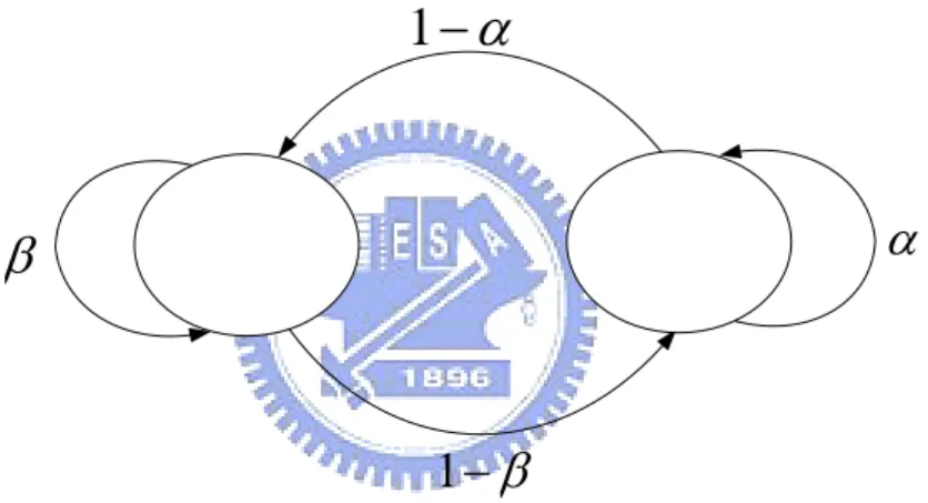
In our thesis, we assume that each mobile has its own channel. Figure 3.2 shows a state diagram for a 2-state Markov model. This model was first used by Gilbert [6] to characterize the error sequences generated by data transmission channels. In the Good state (G) errors occurs with low probability while in the Bad state (B) they occur with high probability.

β

β

−

1

α

−

1

α

Figure 3.2 Gilbert model.

The state transitions are shown in Figure 3.2 and summarized by its transition probability matrix P 1 , 1 P β β α α − ⎡ ⎤ = ⎢ ₋ ⎥ ⎣ ⎦ (3.1) The steady state probabilities of being in states G and B are

β α α τ − + − − = 1 1 1 G and β α β τ − + − − = 1 1 1 B , respectively.

The channel state is either good or bad and can change on packet boundaries, that is, the channel condition stays in a state during one packet duration.

There are some problems here because our channel is “partially observable”. Although the mobile gets the channel state by the return message, it cannot do any action until receiving the next poll from the base station. It must be different for the channel in the time of receiving return message and receiving next poll. That’s the reason why we call the channel “partial observable”.

3.3 Base-station Model

The base-station has two major functions, one is to choose which mobile has the right to transmit at next round, and the other is to be a receiver end.

In the base-station, we assume that for each mobile (ith), there are two attributes

Fi (i=1,2,…N) and tokeni (i=1,2,…N). Fi represents the time when the ith mobile

finishes transmitting packet, and tokeni stands for how many times the ith mobile is

willing to release its transmission right.

A transmission begins from the base-station, the base-station finds the smallest Fi

value, for example Fj, from F1~FN. Then, the base-station checks the value of the

tokenj to see if the value is larger than zero or not. If the value is larger than zero, it

means the mobile is willing to give up its transmission chance at this time. The base-station keep running the cost calculation function to decide which mobile should be polled. On the contrary, if the value is equal to zero, it means the mobile is unwilling to release its chance to transmit. The base-station sends a polling message

to jth mobile and wait for its packet. Combining the results of fair queuing algorithm

with cost calculation function, the base-station decides which mobile can use the channel.

After receiving the packet, it will be passed through a FEC decoder followed by a CRC decoder. We assume a very strong CRC code, with close to 100% error detection capacity. When there are no errors or errors are successfully corrected, an acknowledgement (ACK) is sent back to the sending mobile, and when one or more bit errors are detected by the CRC decoder, and then the base-station returns a negative acknowledgement (NAK) instead of an acknowledgement (ACK). We assume that ACK/NAK messages are highly reliable and take little time that can be negligible.

Assuming that packet errors during a given channel state are independent, the probability that a received packet contains a non-correctable when the channel is in the Good state is given by [5]:

, , , 1 ( ) (1 ) , N i N i T g s g s g i t N p p p i − = + =

∑

− (3.1) , 1 (1 , ) , b s g b g p = − −p (3.2) where p_s,g is symbol error when the channel is in the Good state, and p_b,g is bit error when the channel is in good state.

In the other hand, p_s,b is symbol error when the channel is in the bad state, and

b b

Chapter 4

Problem Formulation Based on MDP

In this section, we formulate our problem to Markov Decision Process. Using the iterative cycle illustrated in Figure 2.3, we can find the optimal policy. The optimal policy is the policy minimizes the total cost, the sum of dropping cost and pushing cost. There are ten kinds of policies, and each of them will make the mobile drop different number of packets before sending packet and transmit packet with different code rate.

We consider the worst case in our work. In the system we assume that the channel is modeled by 2-state time-homogeneous Markov chain and the channel condition does not change during one packet duration.

4.1 State definition

In the previous chapter, we refer to four factors for the method of choosing the policy. So we encode them into one state variable. They are

(5) Prior channel state information (6) Number of successive lost packets (7) The kind of head packet in the buffer

(8) Current number of packets in the mobile buffer

First, the channel information represents the channel condition at last transmission. This information is known through an ACK/NAK message from the base-station. We denote a good condition as 0, and a bad condition as 1

Second, we mention to the number of loss window. If a transmission is successful, the window size will be reset to zero. Else, the window increases because of packet loss or packet error. Packet loss includes the number of dropping packets and the number of pushing packets. We assume that the maximum value of the window is three, so we get four possible states, and they are 0,1,2,3.

Next, we assume that there are four kinds of packets in our system, and the third position represents which kind of packet is going to be sent. The value could be 0,1,2,3.

Last, we suppose the buffer size is finite, and the value is three. Hence, when the buffer size is three, it means the buffer is full. There could be 0,1,2,3 in this position.

Some information only has two possible values, thus it could be indicated using one bit. Some has for possible values, so it takes two bits to represent it. Using these rules, we encode the information into one state as follow:

Figure 4.1 State encoding.

In math equation:

channel+ ×2 window+ ×8 importance+32×buffer=state. (4.1)

By the figure above, we know that we need 7 bits to encoding. Therefore, there are 128 kinds of possible state. Using this scheme, if we want to see the changes of four factors, we simply need to divide the state by the corresponding coefficient.

4.2 Action space

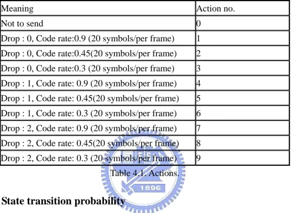
We have ten actions in our action space. Each action is a combination of different code rate and different numbers of early dropping packets. Among all actions, action 0 is a special one, it means we don’t transmit any packet. The possible actions are illustrated in Table 4.1.

Meaning Action no.

Not to send 0

Drop : 0, Code rate:0.9 (20 symbols/per frame) 1

Drop : 0, Code rate:0.45(20 symbols/per frame) 2

Drop : 0, Code rate:0.3 (20 symbols/per frame) 3

Drop : 1, Code rate: 0.9 (20 symbols/per frame) 4

Drop : 1, Code rate: 0.45(20 symbols/per frame) 5

Drop : 1, Code rate: 0.3 (20 symbols/per frame) 6

Drop : 2, Code rate: 0.9 (20 symbols/per frame) 7

Drop : 2, Code rate: 0.45(20 symbols/per frame) 8

Drop : 2, Code rate: 0.3 (20 symbols/per frame) 9

Table 4.1. Actions.

4.3 State transition probability

There are four elements in our state, but not every element affects the transition probability. The pattern of arrival is fixed as 0,1,2,3. As long as we know the importance of current packet, we must know the importance of next packet. Because the pattern is invariable, it doesn’t have any probability distribution. This factor will not influence the state transition probability. On the other hand, the changes of other factors will have effect upon the transition probability.

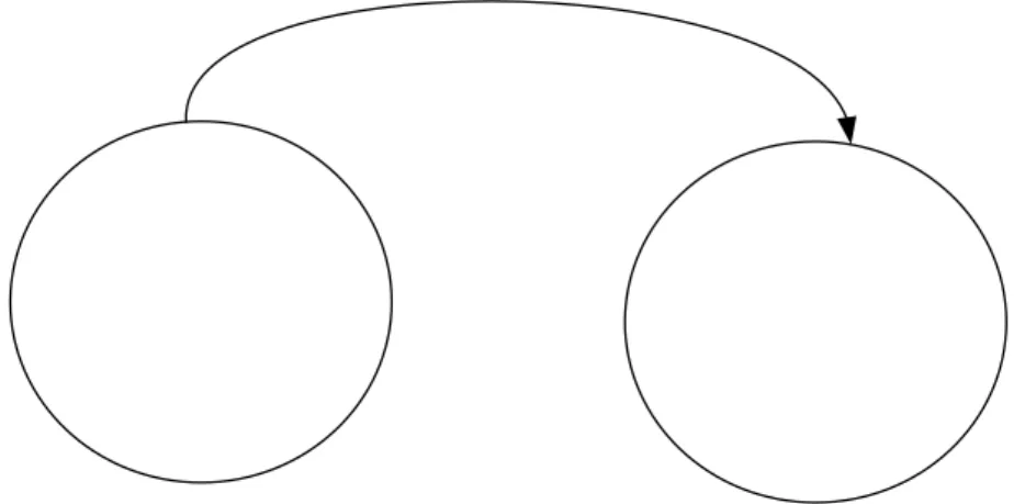
We give an example to specify the effect in the following figure:

Figure 4.2 Transition diagram,

where ptrans(i,j,k) represents the probability of a transition to state j given that the system now occupies state i and takes action k.

The channel status changes from good to bad. Suppose the channel transition probability isprobchannel.

After the mobile took the1 action, next buffer status and the importance of st

packet don’t make any difference but the window value increase. From all these information, we can know what happened at last transmission. The mobile chose the

st

1 action, the action indicates no dropping packets and the code rate of the sending packet is 0.9. Some errors occur in this transmission so the window size increases. Furthermore, there is no arrival during the transmission time thus the buffer length

remains the same. The probability of errors denotesprob_failed and the probability of

no arrival denotesprob_{no arrival_} .

Summarizing above news, we know the state transition probability is calculated by Eq. (4.2):

In some cases, the transmission will be successful, and there will be one arrival

during a transmission time. We replace the term prob_failed with prob_success, and

_ no arrival

prob with prob_{one arrival_} .

If the mobile chooses the 0 action, the mobile will not transmit any packet. th

We only calculate the probability of arrival and probability of channel transition as the following equation:

ptrans(i, j,0) = prob

channel

×

prob

no arrival or one arrival_ ( _ )

.

(4.3)

4.4 Packet cost

Here we only consider the cost due to packet loss. The calculation method relates to the loss window and the importance of the loss packet. Loss of important packets will make huge effects to us. Therefore, even the channel status is bad, we still prefer to transmit the important packet with larger code rate. The equation used to calculate the cost of loss packets is illustrated below:

loss_cost window importance

(

,

)

=

window importance 1

+

+

.

(4.4)

4.5

Cost comparison function

In our system, the base-station has two jobs to do. One is to receive packets from the polled mobile, and the other is to choose which mobile could have the rights to transmit packets.

By [7], we realize the use of additional cost function helping us to minimize the cost of lost calls. We adopt this method in our work. The base-station adopts the fair queuing algorithm first, and then uses this cost comparison function later.

The cost comparison function concerns about the immediate cost and the long term average cost. Within the policy iteration, we call the average loss per transition the “gain”. The immediate cost is defined by the latest action, and the long term

average cost is denoted by the gain obtained from the policy iteration as in chapter 2. We suppose the cost comparison function be a convex combination of the immediate cost and the gain as following equation:

cost(average_cost, gain)=0.5 average cost× _ _{up to now- -} +0.5 gain× (4.5)

4.6 Policy iteration

When finishing the above work, we start to find our optimal policy with the policy iteration described in chapter 2.

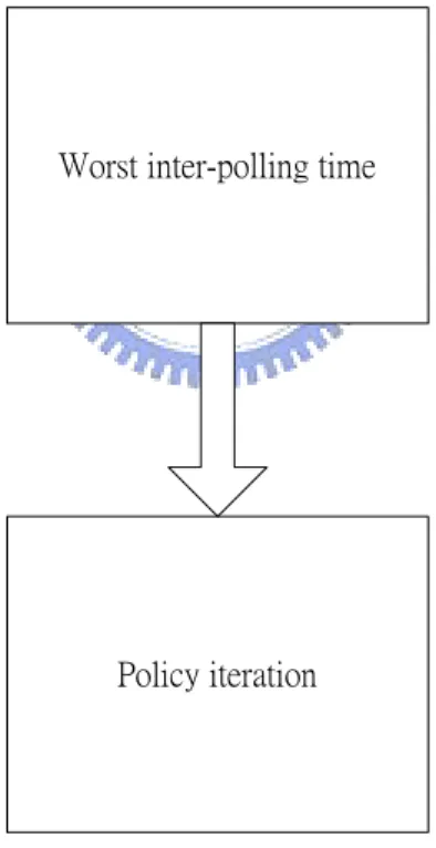
4.7 Worst inter-polling time

Besides the policy iteration, we add another important idea which is the worst polling time into our analysis. In our system, there are 2 mobiles, and they compete for the chance of transmission. At the end of an inter-polling period, the mobile accept a polling message from the base-station, but the length of a inter-polling time is unknown.

We suppose that the channels of two mobiles are independent, the bandwidth for each channel is one symbol per micro-second.

By [8], we can get the inter-polling time in worst case as the following equation:

D

_max

+ b

_max

(np)

,

(4.6)

where Dmax denotes the effective transmission time when the code rate of the

sending packet is maximized, and bmax(np) denotes the maximum transmission time

In Start-Time Fair Queuing algorithm (SFQ), the departure of packet p_fj at the

server, denoted byL_SFQ(p_fj), is given by:

max ( ) ( ) ( , ) . j f j j j n SFQ f f f n Q n f l l C L p EAT p r C C C δ ∈ ∧ ≠ ≤ +

∑

+ + (4.7)

Before the policy iteration we introduced in chapter 2, we calculate the inter-polling time in the worst case. We do the policy iteration within the worst inter-polling time.

Before the policy iteration we introduced in chapter 2, we calculate the inter-polling time in the worst case. We do the policy iteration within the worst inter-polling time.

Worst inter-polling time

Policy iteration

Figure 4.3 Worst case.

Chapter 5

Simulator Design

In this thesis, we will illustrate the parameter and the model setting in our simulation in detail. We suppose that there are 2 mobiles in our simulation.

When each mobile establish the connection with the base station, it will register to the base-station. The mobile runs a MDP algorithm to find an optimal policy before starting transmission. The mobile will choose actions according to the optimal policy.

Here, we assume that the propagation delay is relatively small, so that the ACK/NAK message for a packet is received at the sender end before the next transmission period.

MDP Program and Simulator Setting

The cost is induced by packet loss. We suppose the importance of packets is different, and loss of the most important packet causes most damage. We set cost function as following:

(

,

)

.

loss_cost window importance

=

window importance 1

+

+

(4.4)

The channel of each mobile is independent and has different characteristic. There are two channel states: good and bad. The transition probability matrix is:

0.99

0.01

.1

0.02

0.98

0.98 0.02

.2

0.01 0.99

mobile no

mobile no

⎡

⎤

⎢

⎥

⎣

⎦

⎡

⎤

⎢

⎥

⎣

⎦

A micro-second is a measure of slots. The channel of mobile no.1 becomes bad from good after one slot is 0.01, and it becomes good from bad after one slot is 0.02. In mobile no. 2, the channel becomes bad from good after one slot is 0.02, and it

becomes good from bad after one slot is 0.01, respectively.

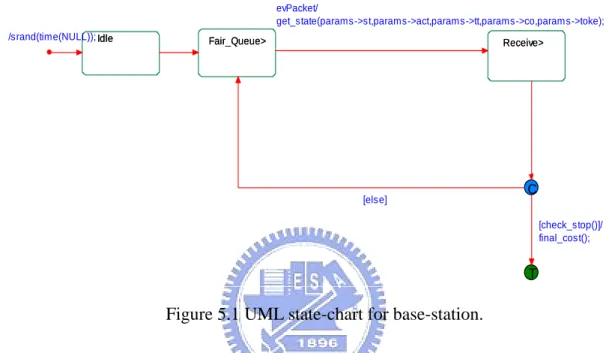
In our simulation, the main part is the base-station, so we introduce its diagram first. The base-station not only plays a role of being a receiver, but also makes a decision to poll a mobile. We describe the state chart of the base-station as the below figure. Fair_Queue> Receive> Idle C T Fair_Queue> Receive> Idle [check_stop()]/ final_cost(); evPacket/ get_state(params->st,params->act,params->tt,params->co,params->toke); /srand(time(NULL)); [else]

Figure 5.1 UML state-chart for base-station.

In “Fair_Queue” block, the base-station performs the fair queuing algorithm. If the token of the chosen mobile is larger than zero, it keeps performing the “compare cost” algorithm to decide which mobile should be polled. After choosing one of the mobiles to transmit packet, the base-station sends the chosen mobile a polling message, then waits the packet arrival. If the base-station gets a packet from the mobile, it checks if the packet data is correct. Depends on correct or not, it feedback an ACK/NAK message.

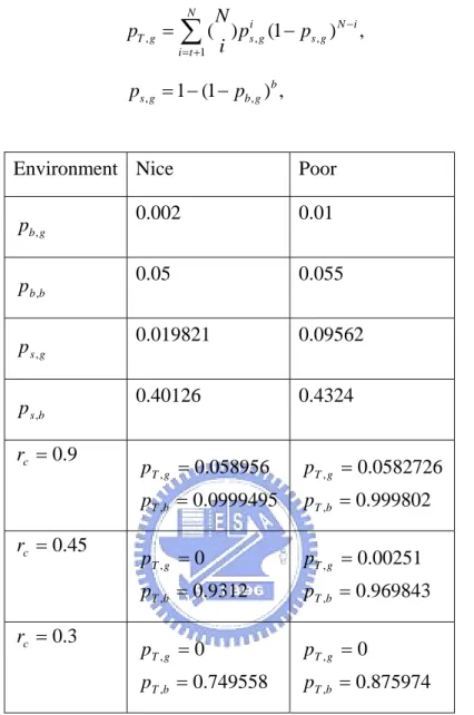
We model our channel as a two-state Markov chain as [5]. Therefore, we can set the bit error probability as it. As chapter 3, the bit error probability in good

environment is denoted byp_b,g , the symbol error probability in good environment is

denoted byp_s,g, and the probability that a received packet contains a non-correctable

when the channel is in the Good state is p_T,g .Using Eq. (3.1) and Eq.(3.2), we

, , , 1 ( ) (1 ) , N i N i T g s g s g i t N p p p i − = + =

∑

− (3.1) , 1 (1 , ) , b s g b g p = − − p (3.2)

Environment Nice Poor

g b p _, 0.002 0.01 b b p , 0.05 0.055 g s p _, 0.019821 0.09562 b s p _, 0.40126 0.4324 9 . 0 = c r 0999495 . 0 058956 . 0 , , = = b T g T p p 999802 . 0 0582726 . 0 , , = = b T g T p p 45 . 0 = c r 9312 . 0 0 , , = = b T g T p p 969843 . 0 00251 . 0 , , = = b T g T p p 3 . 0 = c r 749558 . 0 0 , , = = b T g T p p 875974 . 0 0 , , = = b T g T p p

Table 5.1 Packet error rate in different situation.

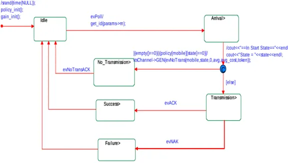
The mobile is on the transmission side, and it chooses action according to the policy from the MDP program. We illustrate its diagram as following figure.

Transmission> Success> Failure> Idle Arrival> No_Transmission> C Transmission> Success> Failure> Idle Arrival> No_Transmission> [(empty()==0)||(policy[mobile][state]==0)]/ itsChannel->GEN(evNoTrans(mobile,state,0,avg,avg_cost,token)); [else]

/cout<<"==In Start State=="<<endl; cout<<"State = "<<state<<endl; evACK /srand(time(NULL)); policy_init(); gain_init(); evNAK evPoll/ get_id(params->m); evNoTransACK

Figure 5.2 UML state-chart for mobiles.

During a inter-polling time, there is either one arrival or no arrival in our simulation. Once it accepts a polling message, it decides the corresponding action. If the buffer is empty or the corresponding action is not to transmit, it follows the “No_Transmission” line. Otherwise, it transmits packets as the code rate which the action decides. Due to the interference over the wireless channel, the packet might be corrupted. If the receiver end can correct the errors or there is no transmission error, then the mobile receives an ACK. Else it receives an NAK instead.

Chapter 6

Simulation results

In this chapter, we illustrate several outcomes from our simulation. Let total transmission rounds be 50 at first, and increase the rounds gradually. We record the total cost at the round end, and the average cost. The total cost is divided by the transmission round to get the average cost. Our goal is to minimize the total cost.

In order to compare the results, we introduce another method called “compare channel”. We use the method we recommend to contrast with this method. Further, we change the calculation functions of cost in two mobiles, and we can see our method is better clearly.

Simulation Results:

We compare the results of the fair queuing algorithm and the method we introduce. From the simulation, we know our method is better. Furthermore, we consider the multi-user diversity issue. We make a contrast with our method and the compare channel method. The compare channel method in the base-station is to choose the mobile with better channel status. In such a case, the performance of our method is also better than the compare channel method.

6.1 Short term Average Cost

In this part, we compare the short term average cost between two methods. One is that the base-station uses the fair queuing algorithm only. The other is it combines the fair queuing algorithm with the compare cost function. The compare cost function is used to choose the mobile with less cost, and the calculation equation is illustrated in chapter 4. The difference between using the fair queuing algorithm only and using additional the compare cost function is clear, but not a very big gap. We can see the difference in the figure below.

Simulation Result of Cost Unchanged 0 0.2 0.4 0.6 0.8 1 1.2 1.4 50 100 150 200 250 300 350 400 450 500 550 600 650 700 750 800 850 900 950 1000 Number of Transmission Av er ag e Co st p er Tr an smi ss io n

fair only cost add

Figure 6.1 Simulation Results of Unchanged Cost (fair queue and cost compare).

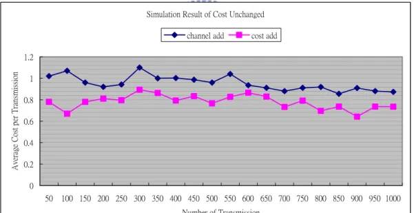
Simulation Result of Cost Unchanged

0 0.2 0.4 0.6 0.8 1 1.2 50 100 150 200 250 300 350 400 450 500 550 600 650 700 750 800 850 900 950 1000 Number of Transmission Av er ag e Co st p er Tr an smi ss io n

channel add cost add

Figure 6.2 Simulation Results of Unchanged Cost (cost compare and channel compare).

In Figure 6.2, we compare the method of compare cost function and the method of compare channel function. Although the later method is always larger than our method, the difference is small. Thus we let the cost function which is used to calculate the cost of packet loss be different in two mobiles. We emphasize the packet cost to see if our method improves the cost of system more than the compare channel function.

We change the cost function in mobile no.2 into the following equation.

(

,

)

(

, )

.

loss_cost window importance

=

window

+

pow importance 2

+

1

(6.1)

And the cost function in the other mobile remains the same as:

(

,

)

.

loss_cost window importance

=

window importance 1

+

+

(4.4)

Simulation Result of Cost Change Case (2)

0 0.2 0.4 0.6 0.8 1 1.2 1.4 1.6 50 100 150 200 250 300 350 400 450 500 550 600 650 700 750 800 850 900 950 1000 Number of Transmission Av er ag e Co st p er Tr an smi ss io n

channel add cost add

Figure 6.3 Simulation Results of Changed Cost Case 2(cost compare and channel compare).

When the cost functions are different in the mobiles, we observe the gap between two methods. The distance is larger than Figure 6.2.

In the next section, we make the loss of the important packet bigger. The gap will become larger. As the previous case, we only change the cost function in one mobile.

The power of the cost function in mobile no.2 increases as Eq. (6.2).

(

,

)

(

, )

.

Simulation Result of Cost Change Case (3) 0 0.5 1 1.5 2 2.5 3 50 _{100 150 200 250 300 350 400 450 500 55}0 ₆₀0 _{650 700 750 800 850 900 950 100}0 Number of Transmission A ver ag e C os t per T ran sm is si on

channel add cost add

Figure 6.4 Simulation Results of Changed Cost Case 3(cost compare and channel compare).

The difference is much clear than the previous one. This tells us when the cost functions are different the effect of using the compare cost function is obvious.

In these cases, we can also get better performances when we use the compare cost function rather than the fair queuing algorithm.

In the case such as only mobile no.2 changes its cost function as Eq. (6.1). We plot Figure 6.5.

Simulation Result of Cost Change Case (2)

0 0.2 0.4 0.6 0.8 1 1.2 1.4 1.6 1.8 2 50 _{100 150 200 250 30}0 ₃₅0 ₄₀0 _{450 500 550 600 650 700 750 800 850 900 950 10}00 Number of Transmission A ver ag e C os t pe r T ran sm is si o

fair only cost add

Simulation Result of Cost Change Case (3) 0 0.5 1 1.5 2 2.5 3 50 _{100 15}0 ₂₀0 ₂₅0 _{300 350 400 450 500 550 600 65}0 ₇₀0 ₇₅0 _{800 850 900} 950 1000 Number of Transmission A ver ag e C os t pe r T ran sm is si on

fair only cost add

Figure 6.6 Simulation Results of Changed Cost Case 3(fair queue and cost compare).

Figure 6.6 is the case we change the cost function in mobile no.2 as Eq. (6.2). In these figure, the distance between two curves becomes larger than Figure 6.1. Difference of the cost function in mobiles not only make the gap between the compare cost method and the compare channel method larger, but also make the discrimination between the fair queuing algorithm and the compare cost function easier.

Long term

In the above figures, the curves don’t seem to be smooth. We want to see the steady state in these cases. We show the average cost in different cases in a long period. The value of the average cost per transmission becomes stable when the number of transmission grows.

6.2 Long term Average Cost

We illustrate the long term average cost in the cases of unchanged cost function and cost function changed as Eq. (6.2).

Simulation Result of Cost Unchanged in Long Period 0 0.2 0.4 0.6 0.8 1 1.2 500 1000 1500 2000 2500 3000 3500 4000 4500 5000 Number of Transmission A ver ag e C os t pe r T ra ns m is si o

fair only channel add cost add

Figure 6.7 Simulation Results of Unchanged Cost (Long Term).

Simulation Result of Cost Change Case (3) in Long Period

0 0.5 1 1.5 2 2.5 500 1000 1500 2000 2500 3000 3500 4000 4500 5000 Number of Transmission Av er ag e Co st p er Tr an smi ss io n

fair only channel add cost add

Figure 6.8 Simulation Results of Changed Cost Case 3 (Long Term).

In Figure 6.7 and Figure 6.8, our method both performs the best. The average cost of the packet loss is much smaller than the other method. And the curves are smooth as the turns of transmitting packets grow.

6.3 Packet Loss Performance

In this section, we discuss the impact of packet loss due to different cost function among mobiles. We keep the cost function unchanged, and observe the outcomes in Figure 6.9. Using our method, packet loss of lower priority is a little higher than other methods. But in the case of higher priority, packet loss is less.

Packet Loss of Cost Unchanged

0.541094 0.28636 0.111699_0.097976 0.558969 0.288606 0.060846 0.570786 0.29659 0.056624 0.087765 0.043985 0 0.1 0.2 0.3 0.4 0.5 0.6 0 1 2 3

Packet Priority (3: Most Important) only fair channel add cost add Normalized Packet Loss

R

Figure 6.9 Packet Loss of Cost Unchanged.

In Figure 6.10, we change the cost function in mobile no.2 as Eq.(6.2). We can get a similar conclusion as above. Moreover, there is one thing to notice. When the cost term affects the cost functions more, higher priority’s packet loss by using the compare channel method increases.