在異質網路上用以改善傳輸控制協定之封包遺失分類演算法

國

立

交

通

大

學

多媒體工程研究所

碩

士

論

文

在異質網路上用以改善傳輸控制協定之封

包

遺

失

分

類

演

算

法

A packet loss classification algorithm to improve TCP

over heterogeneous networks

研 究 生：范竣琇

指導教授：蕭旭峰 教授

在異質網路上用以改善傳輸控制協定之封包遺失分類演算法

學生：范竣琇 指導教授：蕭旭峰

國立交通大學資訊學院

多媒體工程研究所

摘要

A Packet Loss Classification Algorithm to Improve TCP over

Heterogeneous Networks

Student: Jyun-Siou Fan

Advisors：Dr.

Hsu-Feng Hsiao

Institute of Multimedia Engineering

College of Computer Science

National Chiao Tung University

Abstract 

Transmission Control protocol (TCP) is the most widely used transport layer protocol on Internet. As the popularity of wireless communication is on rise over the last few years, TCP is being extended to wireless network. However TCP is not suitable to be used on heterogeneous networks because its congestion control algorithm uses packet loss event as an indicator of network congestion. In a wired/wireless network, there are two classes of packet losses, wireless loss and congestion loss. Wireless loss is caused by common channel errors due to multipath fading, shadowing, and attenuation. Congestion loss is caused by network congestion.

If the congestion control algorithm takes the wireless loss as an index of network congestion, it will mistakenly lead to dramatic performance. In this thesis, we propose a packet loss classification algorithm based on relative one-way trip time (ROTT) and use two trend detections to differentiate congestion loss from wireless loss in the ambiguous area of ROTT distribution.

Then we show that our proposed algorithm can improve network performance comparing with other methods.

Content

摘要 ... i 

Abstract ... ii 

Content ... iii 

List of Tables ... v 

List of Figures ... vi 

Chapter 1 Introduction ... 1 

1.1 Motivation and Introduction ... 1 

1.2 Organization of this thesis ... 2 

Chapter 2 Packet Loss Classification Algorithms ... 3 

2.1 Introduction ... 3 

2.2 Related Packet Loss Classification Algorithms ... 4 

2.2.1 Biaz scheme ... 4 

2.2.2 Spike scheme ... 5 

2.2.3 ZigZag scheme ... 7 

2.2.4 Delay trend scheme ... 8 

2.3 Proposed Method ... 10 

2.3.1 Network Congestion, Packet Loss and ROTT... 10 

2.3.2 Our Proposed Packet Loss Classification Algorithm ... 11 

2.3.3 Discrimination Performance ... 13 

2.3.4 Simulation and Results ... 14 

Chapter 3 TCP Congestion Control Algorithms over Heterogeneous Networks ... 20 

3.1 Introduction to TCP Congestion Control Algorithm ... 21 

3.1.1 Basic Congestion Control Algorithm ... 21 

3.1.2 Discussion on Various TCP Versions ... 26 

3.2 Modified in Response to Wireless Loss ... 33 

3.2.1 The Problem Explanation about TCP over Heterogeneous Networks ... 33 

3.2.2 Some studies to improve TCP over heterogeneous networks... 35 

3.2.3 Modified TCP Congestion Control Algorithm for Wireless Losses ... 37 

Chapter 4 Simulations and Results ... 43 

4.1 The Simulation Environment ... 43 

4.1.1 Performance Metrics ... 43 

4.1.2 Network Parameters ... 44 

4.2 Wireless Error Model ... 44 

4.3 Simulations ... 46 

4.3.1 Simulation results according to different wireless error rates ... 46 

4.3.2 Simulation results according to different traffic ... 55 

Chapter 5 Conclusions ... 59  5.1 Summary ... 59  Reference ... 60 

List of Tables 

Table 1 Accuracy A of TCP1, fixed beta ... 15 

Table 2 Accuracy A of TCP1, fixed alpha ... 15 

Table 3 Accuracy A of TCP1, fixed beta, modified TCP NewReno ... 16 

Table 4 Accuracy A of TCP1, fixed alpha, modified TCP NewReno ... 16 

Table 5 Accuracy comparison, threshold 0.5 ... 17 

Table 6 Accuracy comparison, threshold 0.4 ... 17 

Table 7 Accuracy comparison for topology2 ... 19 

Table 8 Performance comparisons over bottleneck link (error rate 0.034) ... 53 

Table 9 Performance comparisons over bottleneck link (error rate 0.06) ... 53 

Table 10 Performance comparisons over bottleneck link (error rate 0.08) ... 53 

Table 11 Performance comparisons over bottleneck link (error rate 0.12) ... 53 

Table 12 Throughput in the receiver side (error rate 0.034) ... 53 

Table 13 Throughput in the receiver side (error rate 0.06) ... 54 

Table 14 Throughput in the receiver side (error rate 0.08) ... 54 

Table 15 Throughput in the receiver side (error rate 0.12) ... 54 

List of Figures

Figure 2.1 Packet loss classes ... 3 

Figure 2.2 Biaz scheme [5] ... 4 

Figure 2.3 Spike train in Time-ROTT graph [4] ... 5 

Figure 2.4 Spike scheme [5] ... 6 

Figure 2.5 ZigZag scheme [5] ... 8 

Figure 2.6 Delay trend packet loss classification ranges [6] ... 9 

Figure 2.7 Flow chart of our proposed method ... 13 

Figure 2.8 Simulation topology1 ... 14 

Figure 2.9 Simulation topology2 ... 18 

Figure 3.1 TCP header format [8] ... 21 

Figure 3.2 Congestion window variation in slow start and congestion avoidance phases ... 23 

Figure 3.3 Congestion window variation in fast retransmit and fast recovery phases ... 26 

Figure 3.4 The version evolution of TCP ... 27 

Figure 3.5 A sent packets pattern ... 31 

Figure 3.6 The operation process of a TCP NewReno example ... 32 

Figure 3.7: Congestion window variation graph for a TCP NewReno example ... 32 

Figure 3.8 Simple simulation topology ... 34 

Figure 3.9: Compare throughputs between no-wireless-error and wireless-error .... 34 

Figure 3.10 Pseudocode of TCP Westwood algorithm [2] ... 36 

Figure 3.11 A simple example in response to a wireless loss ... 38 

Figure 3.12 A flow chart of TCP control ... 39 

Figure 3.13 Process dupack<3 ... 39 

Figure 3.14 Process dupack>=3 ... 40 

Figure 3.15 Partial_ack action ... 41 

Figure 3.16 Process dupack for fast recovery... 42 

Figure 4.1 A two-state Markov model ... 44 

Figure 4.2 Flow chart of wireless error model ... 46 

Figure 4.3 Simulation topology3 ... 47 

Figure 4.4 Throughput comparisons in bottleneck link ... 48 

Figure 4.5 Throughput comparison of two TCP flows in bottleneck (error rate 0.034) ... 49 

Figure 4.6 Throughput comparison of two TCP flows in bottleneck (error rate 0.06) ... 50 

Figure 4.7 Throughput comparison of two TCP flows in bottleneck (error rate 0.08) ... 51  Figure 4.8 Throughput comparison of two TCP flows in bottleneck (error rate 0.12)

... 52  Figure 4.9 Simulation topology4 ... 55  Figure 4.10 Throughput comparisons in bottleneck link of different traffic

simulation ... 56  Figure 4.11 Throughput comparison of TCP1 in bottleneck of different traffic

simulation ... 56  Figure 4.12 Simulation topology5 ... 57  Figure 4.13 Average throughput in bottleneck link ... 57 

Chapter 1 Introduction 

1.1 Motivation and Introduction 

Transmission Control protocol (TCP) provides a reliable, connection-oriented service and is the most widely used transport layer protocol on Internet. As the popularity of wireless communication is on the rise over the last few years, TCP is being extended to wireless network. However, TCP is not appropriate to be used over heterogeneous (mixed with wired and wireless networks) networks because of the mechanisms of its congestion control algorithm. TCP congestion control algorithm uses packet loss event as an indicator of network congestion. However, there are congestion loss and wireless loss over heterogeneous networks. If the congestion control algorithm takes the wireless loss as an index to network congestion, it will mistakenly lead to dramatic performance degradation. In order to solve this problem, some effective congestion control approaches have been suggested. There are three alternative approaches, end-to-end, localized link layer, and split connection. [1][2]

One of these approaches is to use packet loss classification algorithms to differentiate packet loss classes. According to the classification result, the congestion control algorithm can effectively adjust the sending rate based on the congestion loss instead of wireless loss. Biaz[3] suggested using the inter-arrival time between two consecutive packets to differentiate packet loss as congestion loss or wireless loss. Spike-train [4] is observed on a time-ROTT graph and the packet loss classification method that provides two thresholds based on the relative one-way trip time (ROTT) to differentiate packet loss type. ZigZag scheme [5] discriminates congestion loss from wireless loss using different threshold values of the mean and deviation of ROTT based on the different numbers of lost packets. These methods may cause misclassification of packet loss when the ROTT is around the thresholds. Delay trend scheme

[6] proposed a classification algorithm based on the trend of ROTT to assist packet loss classification in the ambiguous area of ROTT distribution.

In this thesis, we propose a new packet loss classification algorithm. In the ambiguous region of ROTT distribution we also use trend detection method to assist packet loss classification. We implement the decreasing trend detection and also the increasing trend detection for packets in the gray region. Further, with the assistance of this proposed packet loss classification algorithm, we modify TCP congestion control algorithm so that it would perform better over heterogeneous networks.

1.2 Organization of this thesis 

In chapter 2 we review packet loss classification algorithms proposed in last few years in the literature, and propose a new packet loss classification algorithm based on the trend detection of relative one-way trip time. In chapter 3, we describe TCP congestion control algorithm and some variant versions of TCP. We also modify the TCP congestion control algorithm in response to the wireless loss resulting from the packet loss classification algorithm described in the same chapter. In chapter 4, we evaluate the performance of our proposed algorithm and the competing algorithms in the literature, followed by the conclusions in chapter 5.

Chapter 2 Packet Loss Classification 

Algorithms 

2.1 Introduction 

Transmission Control protocol (TCP) is the most widely used transport layer protocol on Internet. As the popularity of wireless communication is on the rise over the last few years, TCP is being extended to wireless network. However TCP was designed to optimize its performance on wired networks, and it is not quite appropriate to be used on either wireless networks or heterogeneous networks. The reason is that TCP congestion control algorithm treats packet loss event as an indicator of network congestion. However in wireless network or heterogeneous networks, there are two classes of packet loss: one is congestion loss, and the other is wireless loss, as shown in Figure 2.1.

Packet losses due to network congestion are called congestion loss. Other kind of packet loss due to shadowing, or signal attenuation over wireless networks is called wireless loss. The intersection of wireless loss and congestion loss in Figure 2.1 means that network suffers from both network congestion and wireless fading.

If the wireless loss is taken as an indicator of network congestion by TCP congestion control algorithm, it will degrade the performance because of the incorrect reduction of the congestion window. The packet loss classification algorithm is introduced to solve this problem. TCP congestion control algorithm only reduces the congestion window in corresponds to the congestion loss differentiated by the packet loss classification algorithm.

In the next section, we review some proposed packet loss classification algorithms in the literature.

2.2 Related Packet Loss Classification Algorithms 

Some packet loss classification algorithms have been proposed recently. In this section we review four packet loss classification methods.

2.2.1 Biaz scheme 

Biaz scheme [3] uses packet inter-arrival time to differentiate congestion loss from wireless loss at the receiver side. Biaz assumes that only the last link along the path is wireless. The wireless link is the bottleneck and the sender performs a bulk data transfer. In this condition the inter-arrival time between two consecutive packets is approximately equal to the time required to transmit a packet on the wireless link. Biaz scheme classifies the packet loss according to the temporal range shown in Figure 2.2.

Figure 2.2 Biaz scheme [5]

Ti denotes the time between the arrivals of the last in-sequence packet and the first

out-of-order packet received after the loss. Tmin denotes the minimum inter-arrival time

(n+2)Tmin, the lost packets are assumed to be lost due to wireless transmission error.

Otherwise the loss event is determined as congestion loss. If the first out-of-order packet arrived around the time that it should be received, we think that the lost packet was transmitted but lost due to wireless channel error. If the first out-of-order packet arrived much earlier than that it should, some packets prior to it are possible to be dropped at the buffer. If it arrives much later than it should, we think that the queuing time at buffers increases. In [3], the accuracy of the classification is determined by the ratio of wired bandwidth and wireless bandwidth, as well as the overall loss rate (congestion loss rate and wireless loss rate). This scheme works best when the last link is wireless link and also the bottleneck link, and it is not shared by other competing traffic. [3][5]

2.2.2 Spike scheme 

In [4], they observed on a time-ROTT graph that relative one-way trip time (ROTT) has an increasing trend, which is called spike-trains as shown in Figure 2.3. They find that congestion-related losses are strongly correlated to the spike-train. Consequently, they use spike-trains instead of packet losses to detect congestion.

Figure 2.3 Spike train in Time-ROTT graph [4]

Spike scheme that classifies packet loss classes can be derived from the phenomenon mentioned above, and it differentiates packet loss type based on relative one-way trip time (ROTT). The ROTT is the time a packet travels from the sender to the

receiver. Since the sender and the receiver might have different clocks, the absolute value of one-way trip time is difficult to calculate, and consequently the relative one-way trip time is used.

Spike scheme defines a state of the connection as spike state according to the ROTT and current state. The spike state is determined as shown in Figure 2.4. The solid line means that the connection is in spike state and the dash line indicates that the connection is not in spike state. If the connection is not in spike state and the ROTT of the packet currently received is larger than the threshold Bspikestart, the connection enters the spike

state. In opposition, if the connection is currently in spike state and the ROTT of the packet received is less than the threshold Bspikeend, the connection leaves the spike state.

Then when the receiver detects a packet loss from a gap in the sequence numbers of received packets, it classifies this packet loss based on the current state of the connection. If the connection is the spike state, the packet loss is classified congestion loss. Otherwise, the packet loss is differentiated as wireless loss.

Figure 2.4 Spike scheme [5]

We calculate the thresholds Bspikestart andBspikeend as shown in equation (2.1) and

(2.2), respectively.

Bspikestart = ROTTmin + α(ROTTmax- ROTTmin) (2.1)

Bspikeend = ROTTmin + β(ROTTmax - ROTTmin) (2.2)

where ROTTmax and ROTTmin are the maximum and minimum relative one-way trip time

The distance between α and β determines the stability of the spike state and non-spike state. The choices of α and β affect the preference of classified congestion loss or wireless loss. For example, if α≧1, congestion loss misclassification rate is 100% while wireless loss misclassification rate is 0%. When α is equal to 1/2 and β is equal to 1/3, this algorithm results in good tradeoff of low congestion loss misclassification and reasonable wireless loss misclassification in the wireless last hop topology mentioned in [5].

2.2.3 ZigZag scheme 

The main idea of ZigZag scheme is that more severe loss is associated with higher congestion and higher ROTT. For this reason, ZigZag increases the classification threshold with the number of losses encountered, as shown in Figure 2.5. That is to say, a loss event that contains four or more lost packets is classified as congestion loss when relative large ROTT is observed. [5]

ZigZag [5] uses different threshold values based on the difference between the mean and deviation of ROTT for different number of lost packets. The mean of ROTT rottmean

and its deviation rottdev are computed by using the equations (2.3) and (2.4) respectively.

The classification boundary of ZigZag scheme is shown in Figure 2.5.

rottmean =(1- α)*rottmean+ α*rott (2.3)

rottdev=(1- 2α)*rottdev+2α*∣rott-rottmean∣ (2.4)

Figure 2.5 ZigZag scheme [5]

A packet loss is differentiated as wireless loss if one of the conditions below is satisfied:

(n=1 AND rotti <rottmean-rottdev)

(n=2 AND rotti < rottmean- rottdev /2)

(n=3 AND rotti < rottmean)

(n>3 AND rotti < rottmean + rottdev /2)

Otherwise, the packet loss is differentiated as congestion loss, as the white portion shown in Figure 2.5.

2.2.4 Delay trend scheme 

A drawback of using threshold on either inter-arrival time or packet ROTT mentioned above is that it is difficult to differentiate congestion loss from wireless loss when either the measured inter-arrival time or measured ROTT is around the distinct boundary, or called as threshold. In the delay trend scheme, an algorithm based on the trend of ROTT to assist packet loss classification in the ambiguous area of ROTT distribution is proposed.

Figure 2.6 Delay trend packet loss classification ranges [6]

When the ROTT of the packet received after a loss occurred is relatively large or relatively small, delay trend scheme could explicitly classify this packet loss as congestion loss or wireless loss respectively. If the ROTT of the packet falls in an ambiguous region, delay trend scheme classifies the packet loss according the variation of ROTT. This ambiguous region in Figure 2.6 is denoted as gray zone to be the interval between TGup and TGlow.

TGup denotes the upper bound of gray zone and TGlow denotes the lower bound of gray zone. TGup and TGlow are computed as equation (2.5) and (2.6) respectively.

TGup = ROTTmin + α(ROTTmax- ROTTmin) (2.5)

TGlow= ROTTmin + β(ROTTmax - ROTTmin) (2.6)

where ROTTmax and ROTTmin are the maximum and minimum of ROTT measured,

respectively. α andβ are the values between 0 and 1, and can control the range of the gray zone.

When the ROTT of the packet received after the packet loss is greater than TGup, the packet loss is classified as congestion; while the ROTT of the received packet is smaller than TGlow, the packet loss is differentiated as wireless loss. If the ROTT of the received packet is in the gray zone, a trend detection process is used to classify packet loss classes.

calculated as shown in equation (2.7).

Sf =(1-γ)* Sf +γ*I(Di>Di-1) (2.7)

where I(X) is defined as 1 if X is valid, and 0 otherwise; Di is the ROTT of the ith packet

andγ is the smoothing factor of Sf.

Sf is the value between 0 and 1. If the ROTT has a strong increasing trend, Sf will

approach 1. Set the threshold of dealy trend Sf,th. If Sf >Sf,th , then the packet is classified

as congestion loss, and as wireless loss otherwise. In [6], delay trend scheme chooses a conservative value Sf,th =0.4.

2.3 Proposed Method 

In this section we propose a new packet loss classification algorithm extended from delay trend scheme. We also exploit the ROTT of received packets to assist packet loss classification, and use trend detection method in the ambiguous region. We add a decreasing trend detection besides the increasing trend detection. Before explaining this new method, we describe the chosen packet loss classification index, ROTT.

2.3.1 Network Congestion, Packet Loss and ROTT 

The relative one-way trip time (ROTT) is defined as the time difference between the sending time and the receiving time, the same as mentioned above. We measure ROTT as the time difference between the receiving time and the packet sending timestamp recorded in packet header plus a fixed bias.

The end-to-end packet delay can be modeled as the summation of propagation delay, queuing delay, transmission delay and router processing delay, as shown in equation (2.8). Propagation delay is the time for the electromagnetic waves to traverse all the link media along the path, and router processing delay is required for the router to multiplex, reassemble, and forward packets. Transmission delay is the time required to send packet

into the link. They are usually constant for a given end-to-end path and the same packet length. The remainder, queuing delay, is the main reason of congestion and leads to packet loss. Therefore we know that packet delay information infers network congestion and packet loss due to network congestion.

T ∑ T _, ∑ P

C ∑ T ,   (2.8)

where Td is the packet delay, Tq,i is the queuing delay of link i, Tp,i is the router

processing delay. Ps is the packet size, and Ci is the capacity of linke i, and this fraction is

transmission delay. The final term is propagation delay and d is the length of physical link and s is the propagation speed in medium.

2.3.2 Our Proposed Packet Loss Classification Algorithm

We use two thresholds TGup and TGlow (defined as equation 2.5 and 2.6) to segment three regions. When ROTT is larger than TGup, it means that ROTT is larger than the time that is required when buffer is filled at level α, we classify the packet loss as congestion loss. Besides, when ROTT is smaller than TGlow, we classify the packet loss as wireless loss. Until this step, the method is the same as the delay trend scheme.

When the measured ROTT falls in the gray zone between TGup and TGlow, we use the trend detection method, “full search”. “Full search” method is used to calculate the trends as shown in equation (2.9) and (2.10).

incr

∑ ∑ I (2.9)

decr

∑ ∑ I (2.10) where I(X) is defined as 1 if X is valid, and 0 otherwise; Di is the ROTT of the ith

packet and w is the search range.

For example, w=5 and the measured ROTT vector = (5 3 5 6 6). The last value ‘6’ means the ROTT of current received packet. If there is an increasing variation from these

two chosen values, then we add one to numerator of the increasing trend. From this example, the first ‘5’ compares with other four values, we could find that there are two increasing variation. The second ‘3’ compares with three values behind it, we could get numerator as 2+3=5. The third ‘5’ compares with two values after it, we could get two increasing variation, and the numerator becomes 2+3+2=7. Adopt the action the same as above, we could get the final numerator as 2+3+2+0=7. The denominator is the number of times we can choose two ROTTs of different lost packets, which is 10 in this case. Then we obtain the increasing trend =0.7. The same as mentioned above, we could also get decreasing trend by detecting the decreasing variation between the arbitrarily two values of w ROTT values. For the last example, we could get the decreasing trend =1/10.

Now we have two trend values: increasing trend (denote as incr_trend) and decreasing trend (denote as decr_trend). Define a threshold as 0.5.

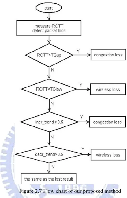
When the ROTT of current received packet falls in the ambiguous area, we compare the increasing trend and decreasing trend with the thresholds. If the increasing trend value is larger than the threshold, we know that ROTTs have an increasing trend and we classify the packet loss as congestion loss. In addition, if decreasing trend is larger than the threshold, we classify the packet loss as wireless loss. Otherwise, ROTT is neither increasing nor decreasing, so we classify the packet loss to be the same as the last packet loss classification result. The flow chart of the proposed method is shown in Figure 2.7.

Figure 2.7 Flow chart of our proposed method

In the next chapter, we will describe TCP congestion control algorithms and how to modify the congestion control algorithm in response to the wireless loss.

2.3.3 Discrimination Performance 

In this section, we use NS-2 to simulate our proposed algorithm and other packet loss classification algorithms, and compare the results between these algorithms. The metrics to evaluate the performance are the accuracy of congestion loss discrimination (Ac), the accuracy of wireless loss discrimination (Aw), and the accuracy of overall discrimination (A). Ac is defined as the ration of the number of congestion losses correctly classified over the total number of congestion losses. Aw is defined as the ration

of the number of wireless losses correctly classified over the total number of wireless losses. A is defined as the ration of the number of total packet losses correctly classified over the number of total packet losses

2.3.4 Simulation and Results 

Our simulation topology is shown in Figure 2.8. Some variables settings, such as link delay and link capacity, are indicated in the figure.

Figure 2.8 Simulation topology1

There are one UDP flow and two TCP flows in our simulation. The UDP flow is from node S0 to node D1 and is attached by a CBR traffic that has 1 Mb sending rate during the time 40 seconds to the time 100 seconds. One of the TCP flows between node S1 and node D1 (denoted TCP1) exists from the time 0 seconds to the time 100 seconds, and the other flow between node S2 and node D2 (denoted TCP2) exists between the time 20 seconds and 100 seconds. Both two TCP flows are FTP. The total simulation time is 100 seconds. The error model of the wireless links, simulated by two-state Markov chain, is turned on at the time 60 seconds and its average error rate is equal to 0.22. More details about this wireless error model will be described in Chap. 4.

A. Effect of different upper bound and lower bound of gray zone

In this simulation, we want to verify the effect of different upper bounds and lower bounds of gray zone on our packet loss classification algorithm. The upper bound and the

lower bound of the gray zone is determined by αand β, as shown in Eq. 2-5 and Eq. 2-6. When β is fixed as 0.1, we change α from 0.99 to 0.7. The sender uses TCP NewReno to control the data sending rate when network is congested.

The required parameters as described in the above sections are listed below: --- Search window: 16

--- The threshold of decrease trend thinc: 0.5

--- The threshold of decrease trend thdec: 0.5

The delay trend scheme is used to be compared with our proposed method and its parameters are set as below.

---γ: 1/16

--- The threshold of delay trend th: 0.5

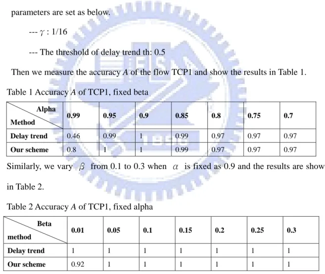
Then we measure the accuracy A of the flow TCP1 and show the results in Table 1. Table 1 Accuracy A of TCP1, fixed beta

Alpha

Method 0.99 0.95 0.9 0.85 0.8 0.75 0.7

Delay trend 0.46 0.99 1 0.99 0.97 0.97 0.97

Our scheme 0.8 1 1 0.99 0.97 0.97 0.97

Similarly, we vary β from 0.1 to 0.3 when α is fixed as 0.9 and the results are shown in Table 2.

Table 2 Accuracy A of TCP1, fixed alpha

Beta

method 0.01 0.05 0.1 0.15 0.2 0.25 0.3

Delay trend 1 1 1 1 1 1 1

Our scheme 0.92 1 1 1 1 1 1

In Table 1, our method shows better accuracies when α is 0.99 or 0.95 and the accuracies form the delay trend scheme and our method get the same results when α is equal to or less than 0.9. Our method gets high accuracy regardless of the very high value of α. When β is larger than 0.05, our scheme and delay trend scheme get stable

accuracies in Table 2. It means that β effects the accuracy of the packet loss classification slightly.

We modify the actions of TCP NewReno in response to the wireless loss and the details about the modification will be described in Chap. 3. The simulation results using the modified TCP NewReno are given in Table 3 and Table 4.

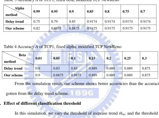
Table 3 Accuracy A of TCP1, fixed beta, modified TCP NewReno

Alpha

method 0.99 0.95 0.9 0.85 0.8 0.75 0.7

Delay trend 0.75 0.79 0.85 0.9174 0.9174 0.9174 0.9174

Our scheme 0.82 0.8875 0.8875 0.9175 0.9175 0.9175 0.9175

Table 4 Accuracy A of TCP1, fixed alpha, modified TCP NewReno

Beta

method 0.01 0.05 0.1 0.15 0.2 0.25 0.3

Delay trend 0.9 0.83 0.85 0.889 0.889 0.889 0.875

Our scheme 0.9 0.8875 0.8875 0.889 0.889 0.889 0.875 From the simulation result, our scheme shows better accuracies than the accuracies gotten from the delay trend scheme.

B. Effect of different classification threshold

In this simulation, we vary the threshold of increase trend thinc and the threshold of

delay trend th from 0.5 to 0.4. According to the simulation results above, we set the parameter α to be 0.8 and the parameter β to be 0.2. Other parameters are the same as above. The modified TCP NewReno is used to control the network congestion.

The simulation results according to different classification thresholds are shown in Table 5 and Table 6.

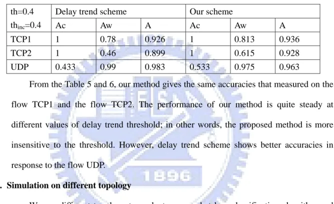
Table 5 Accuracy comparison, threshold 0.5 th=0.5

thinc=0.5

Delay trend scheme Our scheme

Ac Aw A Ac Aw A

TCP1 1 0.831 0.907 1 0.813 0.936

TCP2 1 0.813 0.90 1 0.615 0.928

UDP 0.433 0.996 0.980 0.5 0.979 0.965

Table 6 Accuracy comparison, threshold 0.4 th=0.4

thinc=0.4

Delay trend scheme Our scheme

Ac Aw A Ac Aw A

TCP1 1 0.78 0.926 1 0.813 0.936

TCP2 1 0.46 0.899 1 0.615 0.928

UDP 0.433 0.99 0.983 0.533 0.975 0.963 From the Table 5 and 6, our method gives the same accuracies that measured on the flow TCP1 and the flow TCP2. The performance of our method is quite steady at different values of delay trend threshold; in other words, the proposed method is more insensitive to the threshold. However, delay trend scheme shows better accuracies in response to the flow UDP.

C. Simulation on different topology

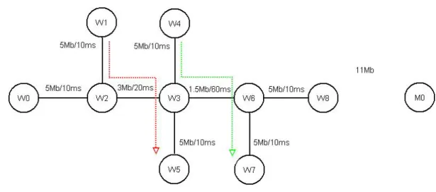
We use different topology to evaluate our packet loss classification algorithm and the delay trend scheme. The new topology is shown in Figure 2.9. The link delay and link capacity are labeled above the link. The wireless link is between node W8 and node M0.

Figure 2.9 Simulation topology2

There are three TCP flows and all of them are FTP. The traffic is setting as following. ---flow TCP1: from node W0 to node M0, 0~100 seconds

---flow TCP2: from node W1 to node W5, 20~60 seconds ---flow TCP3: from node W4 to node W7, 40~80 seconds

The total simulation time is 100 seconds. The error model of the wireless links is turned on at the time 60 seconds and its average error rate is equal to 0.034.

The required parameters about our method and the delay trend scheme are listed below: ---α=0.8

---β=0.2

--- Search window: 16

--- The threshold of decrease trend thinc: 0.5

--- The threshold of decrease trend thdec: 0.5

---γ: 1/16

--- The threshold of delay trend th: 0.5

Table 7 Accuracy comparison for topology2

Ac Aw A

Delay trend scheme 0.58 0.8 0.68 Our method 0.75 0.75 0.75

Our packet loss classification algorithm shows better accuracies and consequently our method is better than the delay trend scheme in this situation.

In the next chapter, we illustrate TCP congestion control algorithm and how we modify the congestion control algorithm in response to the wireless loss.

Chapter 3 TCP Congestion Control 

Algorithms over Heterogeneous 

Networks 

Transmission Control Protocol (TCP) is a transport-layer protocol underneath the application layer. TCP provides a reliable, connection-oriented service to the invoking application. The most fundamental responsibility of TCP is to extend IP’s delivery service between two hosts to a delivery service between two processes running on the host, called transport-layer multiplexing and demultiplexing. TCP also provides error checking by including error-detection field in TCP headers, as the Checksum field shown in Figure 3.1. TCP also provides some other services, such as reliable data transfer and congestion control. TCP ensures that data delivery is successful from the sending process to the receiving process by using the sequence number included in their headers, acknowledgments, and timers. The acknowledgment number field in Fig. 3.1 is also used for providing a reliable data transfer service. The source port and destination port numbers are used for multiplexing and demultiplexing to upper-layer applications. The window field is used for flow control and it indicates the number of bytes that a receiver can accept. The data offset field indicates where the data begins. The reserved field is reserved for future use, and we will use it later. The flag field contains six bits. The RST, SYN, and FIN bits are used for connection setup and teardown. The PSH bit indicates that a receiver should pass the data to the upper layer immediately. The URG bit indicates that there is data in this segment that the sending-side upper-layer entity has marked as ‘urgent’. The urgent point field points to the sequence number of the octet following the urgent data. We describe the basic TCP congestion control

algorithm below. [7]

Figure 3.1 TCP header format [8]

3.1 Introduction to TCP Congestion Control Algorithm 

From RFC2581 [10], there are four phases in the TCP congestion control algorithm: slow start, congestion avoidance, fast retransmit, and fast recovery.

Before describing the congestion control algorithm, we define some variables. The congestion window (cwnd) is a sender-side limit on the amount of data the sender can transmit into the network before receiving an acknowledgment, and the receiver’s advertised window (rwnd) is a receiver-side limit on the amount of outstanding data. The slow start threshold (ssthresh) is used to determine whether the slow start or congestion avoidance phase is used to control data transmission. Furthermore the definitions of some terms that will be used are listed below:

We define a segment as a TCP/IP data packet or an acknowledgment packet. FlightSize: The amount of data that has been sent but not yet acknowledged [10].

Maximum segment size (MSS): The size of the largest segment that the sender can transmit [10].

3.1.1 Basic Congestion Control Algorithm 

In order to avoid congesting the network with an inappropriately large burst of data, the slow start phase is used at the beginning of a transfer, or after repairing loss detected by the retransmission timer.

During the slow start phase, a TCP increments cwnd by a segment for each acknowledgment received that acknowledges new data. Therefore cwnd varies exponentially, for example send one segment, then two, then four, and so on. The slow start phase ends when cwnd reaches ssthresh or when congestion is detected.

2. Congestion avoidance

When cwnd reaches or exceeds ssthresh, the control algorithm will enter the congestion avoidance phase. During congestion avoidance, cwnd is at most incremented by a segment size per round-trip time (RTT). One formula used to update cwnd is given in equation 3.1. [10]

cwnd=cwnd+MSS *MSS/cwnd (3.1) These two phases are implemented together in practice.

From RFC2001 [9], slow start and congestion avoidance combined algorithm operates as follows:

Step1. Initialization for a given connection sets cwnd to one segment and ssthresh to 65535 bytes.

Step2. The TCP output routine never sends more than the minimum of cwnd and the receiver’s advertised window.

Step3. When congestion occurs, one-half of the current window size (the minimum of cwnd and the receiver’s advertised window, but at least two segments) is saved in ssthresh. Additionally, if the congestion is indicated by a timeout, cwnd is set to one segment.

Step4. When new data is acknowledged by the receiver side, increase cwnd, but the way it increases depends on whether TCP is performing slow start or

congestion avoidance.

The slow start phase is used when cwnd is less than or equal to ssthresh. On the other hand, TCP performs congestion avoidance algorithm when cwnd is larger than ssthresh.

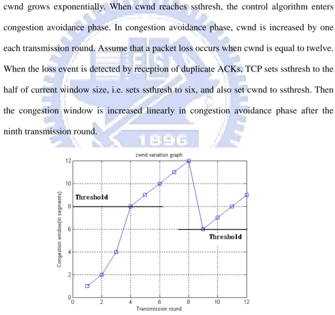
A simple example about congestion window variation in slow start and congestion avoidance phases is given in Figure 3.2. The vertical axis is congestion window and the horizontal axis is the transmission round. Assume ssthresh is eight. First, in slow start phase the congestion window is increased by one each ACK arrived, and consequently cwnd grows exponentially. When cwnd reaches ssthresh, the control algorithm enters congestion avoidance phase. In congestion avoidance phase, cwnd is increased by one each transmission round. Assume that a packet loss occurs when cwnd is equal to twelve. When the loss event is detected by reception of duplicate ACKs, TCP sets ssthresh to the half of current window size, i.e. sets ssthresh to six, and also set cwnd to ssthresh. Then the congestion window is increased linearly in congestion avoidance phase after the ninth transmission round.

3. Fast Retransmit

A TCP receiver should send an immediate duplicate ACK when an out-of-order segment arrives. The purpose of this ACK is to inform the sender that a segment was received out-of-order and which sequence number is expected. [10]

If three or more duplicate ACKs are received by the sender, it is a strong indication that a packet has been lost. So TCP performs a retransmission of the lost packet without waiting for the retransmission timer to expire.

4. Fast Recovery

After fast retransmit phase sends the missing packet, the fast recovery phase is performed to control the congestion window until a non-duplicate ACK arrives. When duplicate ACKs are received, it means not only that a packet loss occurs, but also that packets are mostly leaving the network and received by the receiver. The fast recovery phase is an improvement that allows high throughput under moderate congestion, especially for large windows.

From RFC2581 [10], the fast retransmit and fast recovery algorithms are implemented together as follows:

Step1. When the third duplicate ACK is received, set ssthresh to no more than the value given in equation 3.2.

ssthresh = max (FlightSize/ 2, 2*MSS) (3.2)

Step2. Retransmit the lost segment and set cwnd to ssthresh plus 3*MSS. This artificially "inflates" the congestion window by the number of segments that have left the network and which the receiver has buffered.

Step3. For each additional duplicate ACK received, increment cwnd by MSS. This artificially inflates the congestion window in order to reflect the additional segment that has left the network.

advertised window.

Step5. When the next ACK arrives that acknowledges new data, set cwnd to ssthresh (the value set in step 1). This is termed "deflating" the window.

We describe a simple example in order to understand the operations of fast retransmit and fast recovery. We assume a sent packet pattern whose cwnd is equal to twelve, and the first packet in this window is dropped. According to fast retransmit and fast recovery, we could get the congestion window variation like Figure 3.3. When the third duplicate ACK is received, TCP enters fast retransmit phase, retransmits the lost packet and set cwnd=(12/2)+3=9. Then another packets transmitted in the same window will generate additional duplicate ACKs, so the congestion window is increased in response to these duplicate ACKs. Finally, when the retransmitted packet is received by the receiver, it acknowledges total window of data that is before entering fast retransmit phase. The sender ends the fast recovery phase and sets the congestion window to be equal to six that is half of the congestion window when the packet loss occurs. Then congestion avoidance phase will be used to control congestion window, this operation is the same as the ninth transmission round in Figure 3.2. Namely this cwnd variation in Figure 3.3 occurs in the eighth transmission round of Figure 3.2. When the retransmitted lost packet is received, the eighth round exits, and the ninth round starts.

1 2 3 4 5 6 7 8 9 10 11 12 6 7 8 9 10 11 12 13 14 15 16 17 cwnd variation graph Conges ti on w in dow (i n s egm e nt s )

received packet number

Figure 3.3 Congestion window variation in fast retransmit and fast recovery phases

3.1.2 Discussion on Various TCP Versions   

The two most common reference implementations for TCP are TCP Tahoe, and TCP Reno. In the last section we describe basic TCP congestion control algorithm that refers to TCP Reno. An early version of TCP, TCP Tahoe, unconditionally reduces its congestion window to one segment and enters slow start phase after either type of loss event.( retransmission timer timeout or the receipt of duplicate acknowledges). However TCP Reno, as a modification of TCP Tahoe, enters congestion avoidance phase after the packet loss event indicated by the reception of duplicate ACKs, known as fast recovery. In other words, TCP Tahoe contains slow start, congestion avoidance, and fast retransmit phase, but TCP Reno retains slow start, congestion avoidance, and modifies fast retransmit operation to include fast recovery. [9][13] Since the receiver could only generate the duplicate ACK when another segment is received, it means that there are still data flowing between the sender and the receiver, and consequently TCP doesn’t need to reduce congestion window to one segment. Therefore TCP Reno could get better

performance than TCP Tahoe when packet loss rate is small. However TCP Reno will perform like Tahoe when packet losses are severe; that is to say, it is highly possible that there are multiple packet losses in a single transmission window. [15] The reason for this is as follows. In the last section, we describe that TCP Reno exits fast recovery while the next ACK that acknowledges new data. Even if this ACK just acknowledges some but not all of packets transmitted before the fast retransmit, we would still exit fast recovery and reset congestion window. In this condition it is possible that congestion window is reduced twice for packet losses which occur in a single window, or that if the window is very small when loss occurs then no other additional new packet could be transmitted and we must wait for a timer timeout, and then we retransmit the lost packet and set congestion window to one segment in response to the timeout. This process will cause dramatically performance degradation. [15]

In order to solve this problem, there are some different versions of TCP that has been proposed for TCP/IP protocols, including TCP NewReno, TCP Vegas, and SACK. The version evolution of TCP is drawn in Figure 3.4.

Figure 3.4 The version evolution of TCP

The graph (Figure 3.4) means that TCP New-Reno, TCP Vegas, and TCP SACK are modified versions from TCP Reno.

First, we introduce TCP SACK briefly. TCP with ‘Selective Acknowledgments’ (TCP SACK) is a conservative extension of TCP Reno. It could detect multiple packet

losses of a single window, and retransmit more than one lost packets per round-trip time. This is because that TCP SACK includes a SACK option which permits receiver to inform sender which period of data is not received during transmitting Duplicate ACK. According to the information, TCP SACK sender can know which packet was received and which packet should be retransmitted. [17]

TCP SACK does not change the basic underlying congestion control algorithm. Namely it retains the slow start and congestion avoidance the same as TCP Reno. The main difference between TCP SACK and TCP Reno is in the behavior when multiple packet losses occur in one window. Comparing with TCP Reno, SACK adds a new variable called ‘pipe’ that saves the estimated number of packets outstanding in the path. Using of the ‘pipe’ variable decouples the decision of when to send a packet from which packet to send. [14]

Whenever the sender enters fast recovery, it initializes the variable ‘pipe’. When the sender sends a new packet or retransmits a lost packet, the variable ‘pipe’ is increased by one; pipe is decreased by one each time it receives a ACK with a SACK option reporting that new data has been received by the receiver. When the variable ‘pipe’ is less than the congestion window, it checks the list of packets inferred to be missing at the receiver and retransmits the next packet from the list. If there are no such packets, the sender sends a new packet. Thus more than one lost packet could be sent in one round-trip time. [14] [15]

TCP Vegas not only depend on packet loss as a sign of congestion, but also adopts the difference between expected and actual flow rates to estimate the available bandwidth in the network. Expected flow rate and actual flow rate are defined in equation 3.3 and equation 3.4 respectively. When the network is not congested, the actual flow rate approaches to the expected flow rate. Otherwise, the actual flow rate will be smaller than the expected flow rate. TCP Vegas uses the difference between two flow

rates to estimate network congestion level and varies the congestion window accordingly. [9]

Expected flow rate =

BaseRTT CWND

(3.3) where CWND is the current window size and BaseRTT is the minimum round trip time.

Actual flow rate =

RTT Window

(3.4)

where window means the bytes transmitted between the time that the segment is sent and its ACK is received and RTT is the actual round trip time of a segment.

Especially the variable ‘diff’ is defined in equation 3.5.

diff= (Expected flow rate – Actual flow rate)*BaseRTT (3.5)

TCP Vegas defines two thresholds α and β. If diff is larger than β, Vegas decrease the cwnd linearly during the next RTT, and the sender increase the cwnd linearly when diff is less than α. However if diff is between α and β, Vegas does not change the cwnd.

TCP Vegas tries to keep at least α packets but no more than β packets in the queues. TCP Vegas attempts to utilize the extra bandwidth when it becomes available without congesting the network. However TCP Reno aggressively utilizes available bandwidth.

Before illustrating TCP NewReno, we introduce ‘partial acknowledgment’. When there are multiple packet losses from a single window of data, the retransmitted packet will acknowledge some but not all of the packets before fast retransmit. This acknowledgment is a partial acknowledgment.

TCP NewReno is a modification to the fast recovery algorithm of TCP Reno that incorporates a response to partial acknowledgments received. TCP NewReno defines a “fast recovery procedure” that begins when three duplicate ACKs are received and ends when either a retransmission timeout occurs or an ACK arrives that acknowledges all of

the data up to and including the data that was outstanding at the start of fast recovery procedure. [11]

From RFC2582 [11], TCP NewReno operation is given below.

When the third duplicate ACK is received and the sender is not already in the fast recovery procedure, set ssthresh to be the value given in equation 3.2 and record the highest sequence number transmitted in the variable “recover”.

Step 1.Retransmit the lost segment and set cwnd=ssthresh +3.

Step 2.For each additional duplicate ACK received, increment cwnd by MSS. Step 3.Transmit a segment, if permitted by the new value of cwnd and rwnd. Step 4.When an ACK that acknowledges new data arrives, there are two cases:

Case 1.If it acknowledges all of the data up to and including “recover”, then NewReno exits fast recovery procedure and sets cwnd to ssthresh. Then the congestion avoidance phase is performed.

Case 2.If this ACK is partial acknowledgment, NewReno retransmits the unacknowledged segment. Then reduce the congestion window by the amount of new data acknowledged, add back one segment, and transmit new segment if permitted by the new value of cwnd.

Do not exit the fast recovery procedure. If any duplicate ACKs subsequently arrive, execute step 2 and step 3.

To implement TCP SACK, each acknowledgement is needed to add new blocks that record which segments have been received in the header of acknowledgement. It means that the receiver needs to support the selective acknowledgement. So we don’t take account of using TCP SACK in our simulations.

For TCP Vegas, it is penalized when competing with TCP Reno. When the buffer size increases, TCP Reno throughput increases at the cost of a decrease in TCP Vegas throughput. [16] Namely TCP Vegas is inappropriate to coexist with other versions of

TCP in network.

Because of these reasons above, we finally choose TCP NewReno as TCP version in our simulations.

We illustrate an example below in order to understand TCP NewReno operation in more details. A sent packets pattern is shown in Figure 3.5.

Figure 3.5 A sent packets pattern

Assume the initial congestion window is eight and the receiver’s advertised window is sufficiently large. The first row in Figure 3.5 is packet id. In the second row the symbol ‘O’ means that packet is transferred successfully, and the symbol ‘X’ indicates that packet is dropped. We use TCP NewReno congestion control algorithm to process the packet loss, and to vary the congestion window. The operation process is shown in Figure 3.6.

The node ‘S’ means sender and the node ‘D’ is the destination node. At the third round, the sender receives three duplicate ACKs, and then the congestion control algorithm sets ssthresh=cwnd/2, sets cwnd=ssthreh+3, and retransmit the lost packet.

At the fourth round, it increases the congestion window by the duplicate ACKs number (i.e. cwnd=7+3=10) when the sender receives three additional duplicate ACKs, and transmits two new packets due to the new congestion window. At the fifth round the sender receives a partial ACK, so deflates the congestion window by the amount of new data acknowledged, then add back one. In other words, set cwnd= 10- (4-1)+ 1= 8. At the seventh round the sender receives an acknowledgment which covers the total packets before entering fast recovery, so exit the fast recovery phase, and set cwnd=ssthresh.

Therefore we could get the congestion window variation each time packet is received in Figure 3.7. The horizontal axis is the number of received packets and the

vertical axis is the congestion window.

Figure 3.6 The operation process of a TCP NewReno example

1 2 3 4 5 6 7 8 9 10 4 5 6 7 8 9 10 cwnd variation graph C onges ti on w indow (i n s egm ent s )

received packet number

3.2 Modified in Response to Wireless Loss 

3.2.1 The Problem Explanation about TCP over Heterogeneous 

Networks 

In section 3.1 we describe TCP congestion control algorithm, and learn that TCP congestion control algorithm uses packet losses as an indication of network congestion. Therefore TCP congestion control algorithm limits the sending rate by reducing congestion windows when the sender side detects the packet losses. In RFC 2001 the congestion control algorithm is assumed that packet loss caused by damage is very small, so the loss of packet signals congestion somewhere in the network. This assumption is tenable when the networks are total wired channels, but it is false in heterogeneous networks. The heterogeneous networks mean that the networks contain wired channels and wireless channels. In wireless channel, there are some errors due to shadowing and attenuation that will cause the packet losses. In heterogeneous networks there are two classes of packet losses, one class is caused by network congestion, called congestion loss, and the other class is caused by wireless channel error, called wireless loss.

TCP congestion control algorithm reduces the congestion window regardless of the congestion loss or the wireless loss. This reduction could mistakenly lead to performance degradation.

We simulate a simple example in NS2 environment to verify the statement above. Simulation topology and some parameter setting are shown in Figure 3.8. Node N2 is the base station and the path between node N2, node D1 and node D2 is the wireless link.

Figure 3.8 Simple simulation topology

The simulation has two connections, one is a UDP flow from S1 to D1, and the other connection is a TCP flow between S2 and D2. The UDP flow generates CBR traffic at 1 Mb. We get the throughput results marked as the solid line in Figure 3.8 when no wireless error model is added to the wireless link. Then we add a two-state Markov chain as the wireless error model with average loss rate 22% to the wireless link, and the result is shown as the dash line in Figure 3.9.

0 20 40 60 80 100 120 0 100 200 300 400 500 600 throughput comparison time thr oug hp ut (k b ps ) no error with error

Figure 3.9: Compare throughputs between no-wireless-error and wireless-error

We could find that TCP throughput is dramatically degraded when there are wireless errors in the network, and proof that illustration above.

In order to solve this problem, we use our proposed packet loss classification algorithm to classify the packet loss class, and then modify the TCP congestion control

algorithm in response to the packet losses caused by wireless errors to avoid unnecessarily performance degradation.

3.2.2 Some studies to improve TCP over heterogeneous networks 

TCP is not suitable in heterogeneous networks because of its congestion control algorithm that mentioned above. In order to solve this problem, some effective congestion control approaches for wireless networks have been suggested. There are three alternative approaches, end-to-end, localized link layer, and split connection. The best performing approach is shown to be a localized link layer solution that is applied directly to the wireless links. [13] For example, the protocol called “Snoop” is an approach of link layer solutions. Snoop caches copies of TCP data packets at the base station, and monitor the ACKs from the receiver to the sender. If a packet loss is detected, the cached copy is used for local retransmission across the wireless link, and any packet carrying feedback information back to the TCP sender is extracted to avoid redundant retransmission at the TCP sender. Therefore this protocol could reduce end-to-end retransmission and prevent the associated reduction in congestion window size. However Snoop requires additional supports from base station, and end-to-end methods are promising since significant gains can be achieved without extensive support at the network layer in routers and base stations. [18]

TCP Westwood (TCPW for short) obeys the end-to-end design principle. TCP Westwood is a modified version of TCP Reno. A TCPW sender performs an end-to-end estimate of the available bandwidth along the connection by measuring and averaging the rate of returning acknowledgments. When a packet loss event is observed, that is, a timeout occurs or three duplicate acknowledgments are received, TCPW uses the bandwidth estimate BWE to set the congestion window and the slow start threshold. This procedure is called faster recovery, and the pseudocode of the algorithm is shown in

Figure 3.10. [2] After n duplicate packets are received, the sender modifies the slow start threshold by the measured bandwidth and the minimum relative trip time instead of the half of the congestion window. If the current congestion window is larger than the new threshold, set the congestion window to be the new threshold. If a timeout occurs, set the slow start threshold to be two. The congestion window variations during slow start and congestion avoidance are the same as TCP Reno, that is to say, they increase exponentially and linearly, respectively.

In [2], it shows that TCPW has better throughput than TCP Reno. And TCPW is very effective in handling wireless loss. This is because TCPW uses the current estimated rate as reference to reset the congestion window, but TCP Reno simply halves the congestion window.

Figure 3.10 Pseudocode of TCP Westwood algorithm [2]

Besides TCP Westwood, another aspect of end-to-end approaches is to perform packet loss classification so that the congestion control algorithm can effectively adjust the sending rate based on congestion loss instead of from wireless loss.

In the next section, we illustrate how to modify TCP Reno congestion control algorithm in response to the wireless loss events that are classified by our proposed packet loss classification algorithm. Later we will compare the results of the modified congestion control algorithm using PLC algorithm and TCP Westwood method in chapter 4.

3.2.3 Modified TCP Congestion Control Algorithm for Wireless Losses 

We need to modify the TCP congestion control algorithm in response to the wireless loss. If the receiver detects and classifies a packet loss as the wireless loss by using our proposed packet loss classification algorithm, it sets a flag and records packet loss number in the header of acknowledgment packet in order to inform the sender that wireless losses occur. The number of lost packets is the difference between the discontinuous sequence numbers divided by average packet size.

The flag and packet loss number could be recorded in the reserved field of TCP header (Figure 3.1) in realization. The first bit of the reserved field is used to record the flag. If the flag is set to be 1, it means that the packet loss is a wireless loss; otherwise, the flag is set to be 0. The remainder of the reserved field records the number of the lost packets.

According to the flag and the packet loss number, the sender knows that wireless losses occur and how many packets are dropped, and then use modified congestion control algorithm to vary the congestion window.

In response to wireless losses, we don’t modify the retransmit policy. That is to say, the sender still retransmits the lost packet when three duplicate ACKs are received or timeout of the retransmission timer occurs. However we increase the congestion window as if receiving a new ACK.

For example, assume initial cwnd is equal to six in the slow start phase, and the first packet is lost due to wireless channel error. Then acknowledgment generated due to the second packet in the window could inform the sender that a wireless loss occurs. Then we set new congestion window to eight, i.e. increment like the first packet is received that cwnd is set to seven. A simple chart is shown in Figure 3.11.

Figure 3.11 A simple example in response to a wireless loss

Then we think some complex cases including multiple packet losses in a single window. A flow chart of TCP control is shown in Figure 3.12. In Figure 3.12, the variable “seqno” means the sequence number of the next packet requested by the receiver. In other words, “seqno” is the acknowledgement number in Figure 3.1. The variable “last_ack_” is defined as the acknowledgement number of the last received acknowledgement. The initial value of the variable “recover_” is set to zero. After receiving the third duplicate acknowledgment, the variable “recover_” is recorded as the highest sequence number transmitted, and enter fast recovery phase. The fast recovery phase means that one packet loss has occurred and takes different actions to recovery the successive packet losses in one window.

When the sender receives a packet, it checks whether this packet is a new acknowledgement by comparing “seqno” with “last_ack_”. If “seqno” is larger than “last_ack_”, the control algorithm compares “seqno” with “recover_”. According to the comparison, the control algorithm calls the function “partial_ack action” or the function “recv new ack”. If “seqno” is equal to “last_ack_”, the acknowledgement is a duplicate ack. Then call the function “process dupack for fast recovery” if the control algorithm is in fast recovery phase.

Otherwise, the congestion control algorithm calls the function “process dupack<3” and the function “process dupack>=3” according to the number of the duplicate acknowledgments. The flow in Figure 3.12 is the same as the main flow of TCP NewReno and our modified portion is shown in the following function blocks.

Figure 3.12 A flow chart of TCP control

The flow charts of function “process dupack <3” and function “process dupack >=3” are shown in Figure 3.13 and Figure 3.14. Function “dupack <3” processes the variation of the congestion window when the number of duplicate acknowledgement is smaller than three. The variable “loss_num” is defined as the number of lost packets at the lost event and it is recorded in the acknowledgement header.

If the loss is classified as the wireless loss, cwnd is set to the sum of cwnd, loss_num and one. Otherwise, cwnd is invariable and this action is the same as the control in TCP NewReno.

Figure 3.14 Process dupack>=3

Function “process dupack>=3” process the variation of the congestion window when the number of duplicate acknowledgements is more than or equal to three. The flags “wireless_start”, “c_w” and “w_c” are used to process multiple packet losses in a window.

When the sender receives three duplicate acknowledgements, the control algorithm records the variable “recover_” and enter fast recovery phase. Then check whether the lost packet is a wireless loss or not. If the first lost packet is a wireless loss, “wireless_start” is set to be 1 and set cwnd to be the sum of cwnd, loss_num and one. Otherwise, the control algorithm sets ssthresh to be the half of the current congestion window and sets cwnd to be the sum of ssthresh and 3. A flag in the acknowledgment header is set to be 1 if the loss is a wireless loss or the flag is set to be 0 if the loss is a congestion loss. This flag is maintained for the packets that have the same acknowledgement number until the next packet loss event occurs. According to the variation of the flag, the flags “c_w” and “w_c” are set. When the first loss in a window is a congestion loss and the second loss is a wireless loss, the flag “c_w” is set to be 1.

Similarly, the flag “w_c” is set to be 1 when the first loss in a window is a wireless loss and next loss is a congestion loss. Each time the sender receives a duplicate acknowledgement, the control algorithm updates the flags “w_c” and “c_w”. If the flag “wireless_start” is equal to 1, it means that the first loss in the window is a wireless loss and check whether “w_c” is 1 or not. When “w_c” is equal to 1, a congestion loss occurs after the first wireless loss. Therefore the control algorithm sets cwnd to be increased by one instead of increased by loss_num and records one new variable “newpack”. “newpack” counts the number of the duplicate acknowledgements between the partial ack and the packet after the congestion loss occurs. We use this variable to set new cwnd when the partial ack is received.

If “w_c” is equal to 0, there is no congestion loss and cwnd is set to be the sum of cwnd, loss_num and one.

Figure 3.15 Partial_ack action

If “seqno” is smaller than “recover”, it means that this acknowledgement is a partial ack. The function “partial_ack action” takes actions as shown in Figure 3.15.

If the flag “wireless_start” is equal to 0, the control algorithm takes actions the same as the actions in TCP NewReno. Otherwise, the control algorithm checks the flag “w_c”. When the flag “w_c” is equl to 0, it means there is no congestion loss and cwnd

increases exponentially or linearly according to the relationship between currently cwnd and ssthresh. This action limits the increasing rate of the congestion window and avoids the algorithm occupying excessive bandwidth. If the flag “w_c” is equal to 1, set cwnd to be (cwnd+newpack)/2. The value of the congestion window is (cwnd-newpack) when the congestion loss occurs. So we reset the congestion window to be (cwnd-newpack)/2 in response to the congestion loss. However, the new congestion widow may cause the transmission timer timeout to occur because of the small congestion window. We increase (cwnd-newpack)/2 by “newpack”. Finally, the congestion window is (cwnd+newpack)/2.

Figure 3.16 Process dupack for fast recovery

When the acknowledgement is a duplicate ack and also the TCP congestion control is in fast recovery phase, the function “process dupack for fast recovery” is called. If the acknowledgement is not a wireless loss, the control algorithm increases cwnd by one. Otherwise, cwnd is increased by the sum of “loss_num” and one, in response to the wireless loss.

In the next chapter, the modified TCP congestion control algorithm attached with proposed packet loss classification algorithm is simulated and we compare the simulation results of proposed TCP congestion control with TCP Newreno and TCP Westwood to evaluate the performance of our method.

Chapter 4 Simulations and Results 

4.1 The Simulation Environment 

In this chapter, we use ns-2 as the simulation environment to evaluate the performance of our proposed algorithm, and compare the proposed method with original TCP Newreno and TCP Westwood. In the last chapter we mention TCP Westwood and know that it is also an approach to improve TCP congestion control algorithm. The implementation of TCP Westwood is the modification of TCP Newreno [24].

We choose TCP NewReno as the version of TCP in our simulation and modify it as mentioned in chapter 3. NewReno TCP agent has been implemented in NS-2.

4.1.1 Performance Metrics 

In this section, we describe the performance metrics that we use in this thesis.

Throughput: The important idea of our proposed method is to improve the

throughput degradation from the incorrect control actions when TCP congestion control algorithm is over heterogeneous networks. So the first performance metric is throughput measured in receiver side, and it is defined as the sum of the received packet size in application layer divided by the total simulation time. Beside the throughput in receiver side, we also use other two metrics.

Utility: The second concern is utility of the bottleneck link, and is defined as the

used bandwidth divided by the capacity of the bottleneck link.

Fairness: The last one is fairness between the competing flows and it is defined in

(4.1). [21] (4.1) ) ( ) ( 2 2

∑

∑

Assume that there are n flows, and xi is the resource allocation of flow i.

If all the xi is the same, then fairness is equal to 1.

4.1.2 Network Parameters 

In the simulation all TCP flows are FTP traffic, which corresponds to bulk data transfer. The packet size is fixed at 1,000 bytes. The receiver advised window is large enough so no packet will be dropped at the receiver.

Some packet loss classification related parameters are listed as below: -α: 0.8

-β: 0.2

-Full search window: 16

-Threshold of increase trend: 0.5 -Threshold of decrease trend: 0.5

4.2 Wireless Error Model 

We implement a wireless error model in wireless physical layer of NS2. We choose Gilbert/Elliot’s two-state Markov chain model as the wireless error model in our simulations because Zorzi et al. investigated the error characteristics in a wireless channel, and indicated that two-state Markov model is a good approximation of wireless channel.[23] A state diagram for a two-state Markov model of Gilbert-Elliott channel is illustrated in Figure 4.1.