由電影配樂中探勘音樂情緒之研究 (I)

行政院國家科學委員會專題研究計畫 成果報告

由電影配樂中探勘音樂情緒之研究(第 2 年)

研究成果報告(完整版)

中 華 民 國 97 年 12 月 15 日

行政院國家科學委員會補助專題研究計畫成果報告

由電影配樂中探勘音樂情緒之研究

計畫類別：

;

個別型計畫 □ 整合型計畫

計畫編號：NSC 95－2221－E－004－009-MY2

執行期間：95 年 08 月 01 日至 97 年 07 月 31 日

計畫主持人：沈錳坤

共同主持人：

計畫參與人員：廖家慧、黃詰仁、闕伯丞、邱士銓

成果報告類型(依經費核定清單規定繳交)：□ 精簡報告 ;完整報告

本成果報告包括以下應繳交之附件：

□赴國外出差或研習心得報告一份

□赴大陸地區出差或研習心得報告一份

;出席國際學術會議心得報告

□國際合作研究計畫國外研究報告書一份

處理方式：除產學合作研究計畫、提升產業技術及人才培育研究計畫、列管計

畫及下列情形者外，得立即公開查詢

;涉及專利或其他智慧財產權，□一年;二年後可公開查詢

執行單位：政治大學資訊科學系

由電影配樂中探勘音樂情緒之研究

ABSTRACT

Movies play an important role in our life nowadays. How to analyze the emotional content of the movies becomes one of the major issues. Based on film grammar, there are many audiovisual cues in movies helpful for detecting emotions of scenes. In this research, we investigate the discovery of the relationship between audiovisual cues and emotions of scenes and automatic annotation of the emotion of the scene is achieved. First, the training scenes are labeled with the emotions manually. Second, six classes of audiovisual features are extracted from all scenes. These classes of features consist of color, light, tempo, close-up, audio, and subtitle. Finally, the graph-based approach, Mixed Media Graph approach is modified to mine the association between audiovisual features and emotions of scenes. The experiments show that the accuracy is up to 70%.

1. Introduction

With the development of content digitalization, the increase of computer storage capacity and the raise of network bandwidth, digital video collections grow rapidly in recent years. Instead of time-consuming and tedious manual search for video clips, various techniques for content-based analysis have been developed to automatically analyze and index multimedia data [12][14][16][20].

The purpose of content-based video analysis is to obtain a structured organization of the original video content or to realize its semantics meaning. Content-based video indexing is the task of tagging semantic video units obtained from content analysis to achieve convenient and efficient content retrieval. The techniques for content-based analysis so far enable us to easily access the events, people, objects, and scenes captured by the camera. For example, we can retrieve the most exciting parts of a sport game [12], or to efficiently generate abstracts or summaries of movies or sports game. In addition, multimedia semantic retrieval is getting popular recently. Today, movies play an important role in our life. How to analyze the emotional content of the movies becomes one of major issues.

A film was composed of many elements. Some important aspects in film production are the color composition in the mise-en-scene, lighting, sound, editing, and narrative et al. The relationships

among these elements are a set of informal rules known as film grammar defined in [3] - “the product of experimentation, an accumulation of solutions found by everyday practice of the craft, and results from the fact that films are composed, shaped and built to convey a certain story.” In other words, film grammar embodies film production knowledge that is found more in history of use. It explains the relationships between many cinematic techniques and their semantic meanings delivering to viewer.

From the book – Understanding Movies [10] – every shot and scene in the movies was arranged painstakingly by the director. The director delivers the emotion of the scene to viewer by the way of using different shots, color distribution, lighting, shot cut rate, and sound effect et al. For example, the excitement of a scene increases as the shot length decreases. Other examples include rules about screen movements, cutting on action, colors and variation of lighting effects etc. By exploiting the constraints afforded by the film grammar, high-level affective meaning can emerge from low-level features such as shot length directly. Thus, it offers computable approach in bridging the difficult transition to high-level semantics such as emotions.

As mentioned above, there are many audiovisual cues in movies helpful for detecting emotions of scenes. In this way, we wish to discover the relationship between audiovisual cues and emotions of scenes and then achieve automatic annotation of the emotion of the scene.

Once all scenes are labeled with emotions, users can retrieve the scenes based on its’ prevailing emotion. For instance, users will be able to search for the funniest or the most exciting parts of a movie. In this way, user can save his (her) time to browse this movie. Besides, one application of this research is automatic music accompaniment for scenes. After the emotion of the scene is determined, the emotion is used as the intermediate to find out the related music delivering the same emotion.

In this report, we develop a system grounded upon film grammar to discover the emotions of scenes in film. The Mixed Media Graph algorithm is employed to classify the scenes.

This report is organized as follows. We introduce the related works of affective classification in Section 2. Section 3 describes the audiovisual features used for affective classification. The scene affinity graph used in this research for emotion discovery is elaborated upon Section 4. Experiments and results are presented in Section 5, followed by the conclusion in Section 6.

Nowadays, many approached have been proposed to analyze affective content [11][12][14][15][16][27]. Hanjalic and Xu [11][12][13] exploit motion activity, cut density and sound energy to form the so-called affect curve, which maps to the two-dimensional (Arousal-Valence) emotion model. The affect curve on the two-dimensional model will show us the emotion distribution.

A number of works on affective classification of films have been done. Kang [16] proposed a new technique for detecting affective events such as Fear, Sadness, and Joy using Hidden Markov Models (HMM). He performed empirical study on the relationship between emotional events and low-level features of video content. These low level features consisting of color, motion and shot cut rate were computed for each shot. The feature vector of each shot was transformed to observation vector sequences using vector quantization. He introduced two HMM topologies to detect emotional events. The experiments on six thirty-minute video for emotional event classification show about 70.2% and 78.73 separately.

Based on film theories and psychological models, Wei et al. [39] proposed a color content-based system to analyze the color distribution and related feelings brought to viewers. This system uses a set of color features for color-mood analysis and subgenre discrimination. They introduced two color representations for scenes and full films for extracting the essential moods from the films – Movie Palette Histogram and Mood Dynamic Histogram. Movie Palette Histogram is a global measure for the color palette while Mood Dynamic Histogram is a distinguishing measure for the transitions of the moods in the movie. The dominant color ratio and the pace of the movie are also captured for classification. They exploit eight mood types that are defined by psychologist Plutchik - Anger, Fear, Joy, Sorrow, Acceptance, Rejection, Surprise, and Expectancy. In this paper, emotion and mood are regarded as different concepts. Many emotion terms associated with the eight mood types are selected to describe the eight mood types. Each window consist of six video shots is mapped into a mood type according to the emotions of the six shots. c-SVC Support Vector Machine (SVM) [4] is adopted for mood classification. Their experiments on fifteen full-length films for mood type classification of the window (group of six shots) level show about 80% accuracy.

Wang and Cheong [14] proposed an affective scene classification system that is a complementary approach grounded in the fields of cinematography and psychology. This system exploits a number of effective audiovisual cues and an appropriate set of affective categories that are identified for scene classification. For each scene, the audio and the visual signal were processed separately. The visual signal was segmented into shots (represented as key-frames) to computing visual cues. The audio

signal was separated according to audio type (music, speech, environ or silence). The audio segments then were sent into a support vector machine (SVM) based probabilistic inference machine to obtain high-level audio cues at the scene level. The visual and audio cues were finally concatenated to form the scene vectors, which were sent into the same inference machine to acquire probabilistic vectors. The output of every testing scene is expressed probabilistically and each testing scene was classified into one of the output categories. The overall correct classification rate is 74.69%.

3. Feature Extraction

3.1 Introduction

Critics and scholars categorize movies into three main styles: realism, classicism, and formalism. Rather than separate categories, these three styles might be regarded as a continuous spectrum of possibilities. Realism and formalism are general terms used to describe the movies falling into the two styles’ extremes, while classicism can be viewed as an intermediate style that avoids the extremes of realism and formalism. In other words, few films are exclusively formalist or realist in style [10].

Realistic movies are unapparent in style. What realism directors concern is how to reproduce the surface of reality with little distortion and make their films seems unmanipulated. Such filmmakers use the camera, as a recording mechanism, to describe the subject matters with as little commentary as possible. They care “what is being shown” rather than “how it is manipulated.” Some realists aim for rough look in their movies. Simplicity, spontaneity, and directness are the highest rules.

Formalistic films, on the other hand, are relatively flamboyant in style. Formalism directors are referred to expressionists because their self-expression is at least as important as the subject matter itself. They prefer to express subjective experience of reality. The camera is used to comment on the subject matter, and emphasize its essential rather than its objective nature.

Nowadays, few films are absolutely realistic in style. Most directors use the camera to comment on the subject matter. Even is the famous documentary “Let It Be”, the key reason of people are toughed is how the director present the protagonist’s character.

As we have stated in Section 1, film grammar explains the relationships between many cinematic techniques and their semantic meanings delivering to viewer. A director’s expression is conveyed

In film, the basic film grammar is defined as follows. A film is composed of many scenes, and a scene consists of many shots. A scene is defined as a meaningful story unit while a shot is defined as a stream of many frames continuously recorded by a single camera. Based on how many subject matters or human figures are included within the frame of the screen (not the distance between the camera and the object photographed), most shots can be designed and subsumed under the six basic categories: (1) the extreme long shot, (2) the long shot, (3) the full shot, (4) the medium shot, (5) the close-up, and (6) the extreme close-up. As showed in Table 3.1 [10]. Figure 3.1 shows the examples of shots.

Table 3.1 Six basic categories of shots in cinema [10]

Shot Description

Extreme Long Shot

The extreme long shot is taken from a great distance, sometimes as far as a quarter of a mile away. It is also called “establishing shots” because of being taken at the exterior space, and serve as spatial frames of reference for the closer shots.

Long Shot

Usually, the distance of long shot is between the audience and the stage in the live theater. The closest distance in long shot is equal to full shot that just includes human body in full, with the head near the top of the frame and the feet near the bottom.

Full Shot The distance of full shot is between medium shot and long shot. A full

shot contains over three figures.

Medium Shot

The medium shot contains a figure from the knees or waist up. It is also called “functional shot”, useful for shooting exposition scenes and for dialogue.

Close-Up

The close-up emphasizes little on the background or external location, but on a relatively small object - the human face, for example. The close-up shot enhances the importance of things, often suggesting a symbolic significance by enlarge the size of an object.

Extreme Close-Up

The extreme close-up is a variation of close-up. Therefore, the extreme close-up might show only a person’s eyes or mouth instead of a face.

Figure 3.1 Examples of six kinds of shots in cinema

3.2 Emotion Discovery from Scenes

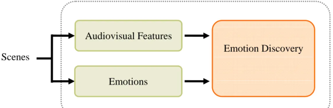
Based on the film grammar, some audiovisual features extracted from films is helpful for the emotion discovery. The relationship between audiovisual features and emotions is close in films. To automatically label the emotion for the query scene, the association between audiovisual features and emotions in films is discovered from training data (scenes). Training data has been labeled of emotions manually. Audiovisual features are extracted from training data. By using these extracted audiovisual features and labeled emotions from training data, the association between audiovisual features and emotions is discovered (Figure 3.2). The discovered association is therefore utilized to label the emotion for the query scene automatically.

Figure 3.2 Association discovery of scenes

close-up medium shot

full shot long shot extreme long shot

extreme close-up

Scenes Emotion Discovery

Audiovisual Features

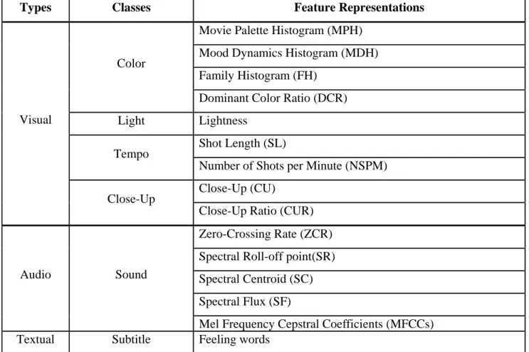
The audiovisual features we adopted consist of several classes of visual features (color, light, tempo, and close-up), one class of audio feature (sound), and one class of textual feature (subtitles). Each class of feature may have more than one feature representation. In total, there are fifteen feature representations which are shown in Table 3.2.

3.3 Visual Features

Visual features include four classes of features – color, light, tempo, and close-up.

Color Class

People are often influenced by color in the subconscious. Psychologists have discovered that most people actively try to interpret the lines of a composition, but they accept color passively, permitting it to suggest moods rather than objects.

Table 3.2 Audiovisual features in our work

Types Classes Feature Representations

Movie Palette Histogram (MPH) Mood Dynamics Histogram (MDH) Family Histogram (FH)

Color

Dominant Color Ratio (DCR) Light Lightness

Shot Length (SL) Tempo

Number of Shots per Minute (NSPM) Close-Up (CU)

Visual

Close-Up

Close-Up Ratio (CUR) Zero-Crossing Rate (ZCR) Spectral Roll-off point(SR) Spectral Centroid (SC) Spectral Flux (SF) Audio Sound

Mel Frequency Cepstral Coefficients (MFCCs)

Visual artists have used color for symbolic purposes for a long time. Though Color symbolism is dependent on cultural, in general, cool colors (blue, green, violet) tend to suggest tranquility, aloofness, and serenity. Warm colors (red, yellow, orange) suggest aggressiveness, violence, and stimulation [10]. “Life is beautiful”, for example, the movie starts from funny scenes, the color is bright and warm, but when the massacre begin, the color of movie starts receding from images.

In the color feature, we adopt four color representations used in [23] - Family Histogram (FH), Movie Palette Histogram (MPH), Mood Dynamics Histogram (MDH), and Dominant Color Ratio (DCR). We modify them as follows,

y Family Histogram: It is a shot level feature, defined as the color histogram of a shot’s key-frame. One key-frame is used to represent one shot.

­ Family Histogram H of the shot k: k

∑

where Pix(x, y) is the pixel value of position (x, y) in the key frame of the shot k ; i is a bin number in CIELUV color space, i = 1 ~ 264;

y Movie Palette Histogram: MPH is a scene level feature in the scene view. It is defined as the color histogram of twelve reference colors in one scene. Main colors of a scene can be captured from MPH.

1) Before computing MPH, we first compute Dominant Color Palette : ) ( k DCP of the shot k, ] , , [ ) ( 1 2 3 k k k P P P k

DCP = , for k = 1 ~ N. N is the number of shots in the scene.

where P1k, k

P2 , k

P3 are the three bin numbers of corresponding top three dominant colors in

histogram H . k } ] ) ( [ max { arg 264 ~ 1 1 H i P k i i k = = ⎪⎩ ⎪ ⎨ ⎧ > × = otherwise Th P H P H if P P k k k k k k , 0 ] ) ( [ ) ( , _{2 1} 2 2

⎪⎩ ⎪ ⎨ ⎧ > × = otherwise Th P H P H if P P k k k k k k , 0 ] ) ( [ ) ( , _{3 2} 3 3

where Th : 0~1, a fixed threshold.

2) After computing Dominant Color Palette, we can get dominant color bin counts :

) ( ₁ 1 k k k P H D = ⎪⎩ ⎪ ⎨ ⎧ > × = otherwise Th P H P H if P H D k k k k k k k , 0 ] ) ( [ ) ( , ) ( 2 2 1 2 ⎪⎩ ⎪ ⎨ ⎧ > × = otherwise Th P H P H if P H D k k k k k k k , 0 ] ) ( [ ) ( , ) ( 3 3 2 3

where Th : 0~1, a fixed threshold.

3) Based on dominant color, Representative Dominant Color Sequence for the shot k , RDCS( k), is defined as:

∑

4) Next, we get Movie Palette (MP):

}

]

)

)

(

,

)

(

(

[

min

{

arg

)

(

m

R

k

RDCS

dis

k

MP

=

)

(m

R

*)

(*,

dis

5) Finally, MPH is derived from MP:

∑

y Mood Dynamics Histogram: MDH is a scene level feature. Color transitions between shots may lead to mood dynamics [23]. We acquire MDH from the statistics of color transitions in movie palette.

­ MDH((m1−1)×12+m2)= ∑ = ⎪ ⎪ ⎩ ⎪ ⎪ ⎨ ⎧ ≠ = = − = = = − N k otherwise m m m R k MP m R k MP if m m m R k MP m R k MP if N 2 1 2 1 2 2 1 2 1 , 0 ] [ & ] ) ( ) ( [ & ] ) ( ) 1 ( [ , 1 ] [ & ] ) ( ) ( [ & ] ) ( ) 1 ( [ , 1

for m1 = 1 ~ 12, m2= 1 ~ 12, where N is the number of shots in the scene.

y Dominant Color Ratio: Dominant color ratio is a shot level feature. While MPH signifies main

colors, DCR indicates the degree of influence of main colors in a shot. In other words, the higher DCR the shot has, the more representative the main colors are in this shot.

­ Dominant Color Ratio :

| | | | P P DCR= d

where P is the set of dominant color pixels, and P is the set of all pixels in a frame. d

Light Class

Light and dark have had symbolic meanings from the dawn of humanity. Light suggests security, justice, and joy. Dark, however, is borrowed to suggest fear, evil, and the unknown. There are various styles of lightings according to different themes and moods of films. In general, comedies tend to be lit in “high key” with bright and little shadows. Mysteries and thrillers are generally in “low key”, with diffused shadows and atmospheric light. Tragedies are usually lit in “high contrast” with harsh shafts of lights and dramatic streaks of blackness.

y Lightness: Lightness is the only representation of the light feature. Lightness is defined as the average luminance of the shot’s key-frame.

Tempo Class

From the cinematographic perspective, the pace is manipulated to great effect by editing effects like cuts. As each shot conveys an event, the filmmaker can intensify a scene by increasing the event density via rapid shot changes [40]. To the viewer, rapid shot changes capturing the main action from different angles certainly convey the dynamic and breathtaking excitement far more effectively than a long duration shot [33] [2].

The tempo feature consist of two representation, Shot Length (SL) and Number of Shots Per Minute (NSPM), defined as follows,

y Shot Length: Shot length is defined as the number of frames in the shot.

y Number of Shots Per Minute: NSPM is a scene level feature, defined as the number of shots per

minute in the scene. The more shots one scene has in a minute, the more excited the audiences feel.

Close-up Class

It is essential for a filmmaker to concern what kind of shot to use to convey the action of a scene. When we see a close-up of the character, it implies that the filmmaker forces us to care about him or her and to identify with his or her feelings. If the character is a villain, the close-up shot can make an emotional revulsion in us. For example, when a threatening character is so close to us, he seems to encroach on our space.

Generally speaking, the greater the distance between the objects and the camera, the more emotionally neutral we remains. One of Chaplin’s most famous pronouncements is “Long shot for comedy, close-up for tragedy”. This principle appears to make sense for when an action “a person is slipping on a banana peel” is close to us, it’s hardly funny because the person’s safety will become our first concern. But if we see this event from a greater distance, it seems to be a comical act to us.

The close-up feature comprises Close-Up and Close-Up Ratio (CUR) representations.

y Close-Up: it describes whether the shot is a close-up. Close-Up for shot k:

­ ⎩ ⎨ ⎧ − − = − . , 0 . , 1 ) ( up close a not is shot the if up close a is shot the if k Up Close

y Close-Up Ratio: CUR is a scene level feature. Because the audience have an inclination toward

identification with the character in a close-up, close-up ratio may be helpful in determining emotion of the scene. CUR is defined as follow:

­ scene the in shots of number Total scene the in up close of number The Ratio Up Close− = −

3.4 Audio Features

Sound plays a very essential role in films. In sound, sound effect and music are the most influential on the audience emotion. Famous director Akira Kurosawa had said “Cinematic sound is that which does not simply add to, but multiplies, two or three times, the effect of the image.” Although the emotion of audience is usually governed by sounds in films, they are often not aware of it.

Sound Effect

Sound effects can be precise source of meaning in film. The pitch, tempo, and volume of sound effects strongly arouse various emotions of the audience. As high-pitched sounds are usually strident and create a sense of tension, they are often employed in suspense scenes especially just before and during the climax. Low-frequency sounds, on the other hand, are usually used to emphasize the grandeur or solemnity of a scene as their heaviness and fullness. In addition, low-pitched sounds can also suggest anxiety and mystery. For example, usually, a suspense sequence usually borrows the low-pitched sounds first, and gradually turns the sounds to be high-pitched as the scene moves toward its climax.

This is not absolute principle though for silence can be powerful sometimes. In sound movies, complete silence for few minutes or even few seconds can suspend the audience and draw their considerable attention. Moreover, as we tend to fear what we can’t see, the filmmakers sometimes prompt a sense of terror in the audience by using off-screen sound effects in horror or suspense films.

Music

In general, music with lyrics is pretty influential since music itself and words convey meanings. However, accompanied with film images, music, no matter with or without lyrics, can be more specific. The theme of a film is usually implied from the cinematic music in the opening. If the filmmaker does not provide the audience with a scene for the dramatic climax, music serves as a foreshadowing. Such hint as Hitchcock, following anxious music, can be one of the warnings to the audience to be prepared. Directors sometimes mislead the audience deliberately by using false musical warnings. Similarly, we can tell actors’ internal emotion by music when actors are required to assume neutral expressions.

We exploit five audio feature representations that are widely used for audio classification and speech recognition.

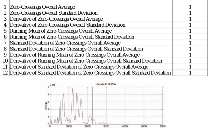
y Zero-Crossing Rate: ZCR is a basic acoustic feature that is defined as the number of times the signal value crosses the zero axis in time domain within a frame [36]. ZCR is proved to be useful in characterizing distinct audio signals. It has been popularly used in speech/music classification algorithms [22]. As shown in Figure 3-3, periodical sound tends to have a smaller value of ZCR, while noisy sound tends to have a higher value. Table 3.3 shows the twelve statistics of ZCR in our work.

Figure 3.3 Zero-crossing rate during voiced speech region (top, ZCR = 432) and unvoiced speech region (button, ZCR = 7150) [31]

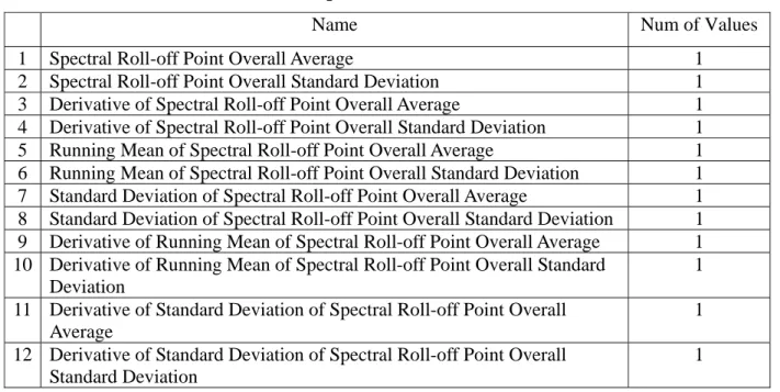
y Spectral Roll-off point: spectral roll-off point is the frequency below which 95th percentile of the power in the spectrum resides [37]. This is a measure of the "skewness" of the spectral shape - the value is higher for right-skewed distributions [37]. SR can tells voiced speech from unvoiced speech as unvoiced speech has a high proportion of energy contained in the high-frequency range of the spectrum, while most of the energy for unvoiced speech and music is contained in lower bands of spectrum. Table 3.4 shows the twelve statistics of SR in our work. Figure 3.4 shows the energy spectrum (cumulative energy) along frequency with 95% spectral roll-off frequency. The spectral roll-off value for a frame is computed as follows:

­

∑

∑

=

=

f

E

f

E

where

K

SR

,

[

]

0

.

95

[

]

E[f] is the energy of the signal at the frequency f.

fMAX is the maximal frequency in the spectrum.

Table 3.3 Zero-Crossing Rate statistics

Name Num. of values

1 Zero-Crossings Overall Average 1

2 Zero-Crossings Overall Standard Deviation 1

3 Derivative of Zero-Crossings Overall Average 1

4 Derivative of Zero-Crossings Overall Standard Deviation 1

5 Running Mean of Zero-Crossings Overall Average 1

6 Running Mean of Zero-Crossings Overall Standard Deviation 1

7 Standard Deviation of Zero-Crossings Overall Average 1

8 Standard Deviation of Zero-Crossings Overall Standard Deviation 1

9 Derivative of Running Mean of Zero-Crossings Overall Average 1

10 Derivative of Running Mean of Zero-Crossings Overall Standard Deviation 1

11 Derivative of Standard Deviation of Zero-Crossings Overall Average 1

12 Derivative of Standard Deviation of Zero-Crossings Overall Standard Deviation 1

Figure 3.4 [Top] Energy spectrum along frequency with 95% spectral roll-off frequency (vertical red line) [bottom] cumulative energy along frequency with 95% spectral roll-off frequency

Table 3.4 Spectral Roll-off point statistics

Name Num of Values

1 Spectral Roll-off Point Overall Average 1

2 Spectral Roll-off Point Overall Standard Deviation 1

3 Derivative of Spectral Roll-off Point Overall Average 1

4 Derivative of Spectral Roll-off Point Overall Standard Deviation 1

5 Running Mean of Spectral Roll-off Point Overall Average 1

6 Running Mean of Spectral Roll-off Point Overall Standard Deviation 1

7 Standard Deviation of Spectral Roll-off Point Overall Average 1

8 Standard Deviation of Spectral Roll-off Point Overall Standard Deviation 1

9 Derivative of Running Mean of Spectral Roll-off Point Overall Average 1

10 Derivative of Running Mean of Spectral Roll-off Point Overall Standard Deviation

1

11 Derivative of Standard Deviation of Spectral Roll-off Point Overall Average 1

12 Derivative of Standard Deviation of Spectral Roll-off Point Overall Standard Deviation

1

y Spectral Centroid: the “balancing point” of the spectral power distribution. Many types of music involve percussive sounds which push the spectral mean higher by including high-frequency noise [37]. The spectral centroid for a frame is computed as follows:

­ ∑ ∑ ⋅ = k k k X k X k SC ] [ ] [

Where: k is an index corresponding to a frequency, or small band of frequencies within the overall measured spectrum, and X[k] is the power of the signal at the corresponding frequency band. Table 3.5 shows the twelve statistics of SC in our work.

y Spectral Flux statistic: the average variation value of spectrum between the adjacent two frames in one second window [21]. Table 3.6 shows the twelve statistics of SF in our work.

­

where X means the magnitude of FFT coefficients.

N is the number of frames in one window.

δ is a little value to avoid log zero.

Table 3.5 Spectral Centroid statistics

Name Num of Values

1 Spectral Roll-off Point Overall Average 1

2 Spectral Roll-off Point Overall Standard Deviation 1

3 Derivative of Spectral Roll-off Point Overall Average 1

4 Derivative of Spectral Roll-off Point Overall Standard Deviation 1

5 Running Mean of Spectral Roll-off Point Overall Average 1

6 Running Mean of Spectral Roll-off Point Overall Standard Deviation 1

7 Standard Deviation of Spectral Roll-off Point Overall Average 1

8 Standard Deviation of Spectral Roll-off Point Overall Standard Deviation 1

9 Derivative of Running Mean of Spectral Roll-off Point Overall Average 1

10 Derivative of Running Mean of Spectral Roll-off Point Overall Standard Deviation

1 11 Derivative of Standard Deviation of Spectral Roll-off Point Overall

Average

1 12 Derivative of Standard Deviation of Spectral Roll-off Point Overall

Standard Deviation

1

Table 3.6 Spectral Flux statistics

Name Num of Values

1 Spectral Flux Overall Average 1

2 Spectral Flux Overall Standard Deviation 1

3 Derivative of Spectral Flux Overall Average 1

4 Derivative of Spectral Flux Overall Standard Deviation 1

5 Running Mean of Spectral Flux Overall Average 1

6 Running Mean of Spectral Flux Overall Standard Deviation 1

7 Standard Deviation of Spectral Flux Overall Average 1

8 Standard Deviation of Spectral Flux Overall Standard Deviation 1

9 Derivative of Running Mean of Spectral Flux Overall Average 1

10 Derivative of Running Mean of Spectral Flux Overall Standard Deviation 1

11 Derivative of Standard Deviation of Spectral Flux Overall Average 1

12 Derivative of Standard Deviation of Spectral Flux Overall Standard Deviation

1

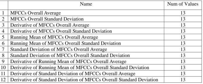
y Mel Frequency Cepstral Coefficients (MFCCs): MFCCs is the feature popularly used for speech

recognition and audio classification due to it's effectiveness in representing the spectral variations of audio. The MFCCs stands for the shape of the spectrum with few coefficients. The cepstrum is the Fourier Transform (or Discrete Cosine Transform DCT) of the logarithm of the spectrum. Instead of the Fourier spectrum, the Mel-cepstrum is the cepstrum computed on the Mel-bands. By using of the

coefficients of the Mel cepstrum. MFCCs are commonly derived as follows: 1. Take the Fourier Transform of (a windowed excerpt of) a signal.

2. Map the log amplitudes of the spectrum obtained above onto the mel scale, using triangular overlapping windows.

3. Take the Discrete Cosine Transform of the list of mel log-amplitudes, as if it were a signal. 4. The MFCCs are the amplitudes of the resulting spectrum.

Table 3.7 shows the twelve statistics of MFCCs in our work.

Table 3.7 MFCCs statistics

Name Num of Values

1 MFCCs Overall Average 13

2 MFCCs Overall Standard Deviation 13

3 Derivative of MFCCs Overall Average 13

4 Derivative of MFCCs Overall Standard Deviation 13

5 Running Mean of MFCCs Overall Average 13

6 Running Mean of MFCCs Overall Standard Deviation 13

7 Standard Deviation of MFCCs Overall Average 13

8 Standard Deviation of MFCCs Overall Standard Deviation 13

9 Derivative of Running Mean of MFCCs Overall Average 13

10 Derivative of Running Mean of MFCCs Overall Standard Deviation 13

11 Derivative of Standard Deviation of MFCCs Overall Average 13

12 Derivative of Standard Deviation of MFCCs Overall Standard Deviation 13

3.5 Textual Feature

Monologue and dialogue are two types of spoken languages in films. Monologue happens when the character talks to self or the off-screen person narrates the background story to facilitate our understanding about the scene or the film. Dialogue can be the conversation among more than two actors.

The textual feature for each scene is defined as a set of the feeling words appearing in the caption stream of the scene. The feeling word list we used for textual feature extraction is collected by Hein [42]. There are over 3000 words in total. We divided these feeling words into two classes – positive and negative feelings for similarity measure. Each feeling word belongs to one class.

In this section, we will introduce the output emotion categories we used in this report, the graph-based algorithm – Mixed Media Graph (MMG) and two topologies revised from MMG will also be introduced.

4.1 Emotion Taxonomy

Affective perception includes emotion, feeling, and mood. Emotion and feeling are different responses. Emotion is directed outwards whereas feeling is inward [6]. Also, emotion and mood are different concepts. Emotion is aroused by some events or objects and usually lasts for a few minutes, while mood is an emotional state and lasts for a longer period of time compared with emotion [17].

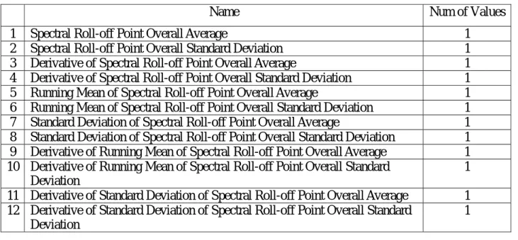
Many emotion models were proposed in psychology. For dimensional approach to describe emotions, VAD is the most popular model proposed by Osgood et al. [26] and also Russell and Mehrabian [34]. The VAD comprises three basic dimensions: Valence, Arousal, and Dominance. Valence is characterized as a continuous range of affective responses or states ranging from pleasant to unpleasant, while Arousal is characterized by affective states ranging on a continuous scale from excited to calm. We can also say that Arousal stands for the “intensity” of emotion, while Valence stands for the “type” of emotion. The third dimension – Dominance – is useful to distinguish between emotional states with similar Arousal and Valence (e.g., “grief” and “rage”) and ranges from “no control” to “full control”. Therefore, the entire scope of human emotions can be represented as a set of points in the three-dimensional VAD coordinate space, as shown in Figure 4.1. The influence of Dominance, however, is truly small so that the control dimension can be ignored. Consequently, the emotion space is reduced to the projection of three-dimensional surface onto the arousal-valence plane as shown in Figure 4.2.

Figure 4.2 Illustration of the 2-D emotion space (from Dietz and Lang [7])

Thayer [38] adapted Russell's model to divide music mood into four classes based on a two-dimensional Energy-Stress mood model. The Energy dimension corresponds to the arousal, while Stress corresponds to valence in Russell’s model. As shown in Figure 4.3, Contentment refers to happy and calm music, such as Bach’s “Jesus, Joy of Man’s Desiring”; Depression refers to tired and tense music, such as the opening of Stravinsky’s “Firebird”; Exuberance refers to happy and energetic music such as Rossini’s “William Tell Overture”; and Anxious/Frantic refers to tense and energetic music, such as Berg’s “Lulu”.

Figure 4.3 Illustration of Thayer’s two-dimensional mood model [38]

Based on human facial expressions of emotion, Ekman [9] identified the six basic emotions: Happy,

Ortony et al. [25] proposed an emotion model based on the assumption that an emotion is a reaction to events (pleased versus displeased), agents (approving versus disapproving) or objects (liking versus disliking). There are twenty-two emotions in this model: Happy-for, Resentment, Gloating, Pity, Hope,

Fear, Satisfaction, Fears-Confirmed, Relief, Disappointment, Joy, Distress, Pride, Shame, Admiration,

Reproach, Gratification, Remorse, Gratitude, Anger, Love, and Hate.

In our work, we mainly use the emotion categories proposed by Wang and Cheong [14]. In order to fit emotion categories for film domain application, Wang et al modified Ekman’s six basic emotions as follows:

1. Disgust is dropped due to the lack of scenes that seek to evoke “pure” Disgust. In addition, scenes that evoke Disgust often contain a strong element of Fear.

2. Add a Neutral emotion category to emotion list because many scenes in films are emotionally neutral. 3. Partition Happy emotion category into Joyous and Tender Affections. Happy includes many sub-families of positive feelings because these sub-families don’t have their own unique facial expression besides smiling expression. Therefore, it is useful and cinematically relevant to partition

Happy.

Therefore, the emotion categories are Joyous, Tender Affections (abbreviated as TA), Anger, Sad,

Fear, Surprise, and Neutral. This set obeys the following four criteria and is appropriate for

scene-level content in film:

1) Universality: Each emotion can be universally realized and experienced. 2) Distinctiveness: Each emotion is clearly discriminated from the other. 3) Utility: Each emotion should have significant relevance in the film context.

4) Comprehensiveness: This emotion set should be adequate to describe almost all emotions in films.

4.2 Mixed Media Graph (MMG)

After extracting audiovisual features, we use Mixed Media Graph [29] to discover the emotion for the query scene. MMG is a graph-based approach used to find correlations across the media in a collection of multimedia objects. Through MMG, the association between audiovisual features and emotions in scenes can be discovered.

The problem and assumption of MMG are defined as follows:

PROBLEM 4.1: Given a set S of n multimedia objects S = {O1, O2, … , On}, each with m multimedia

DEFINITION 4.1: The domain Di of (set-valued) attribute i is the collection of atomic values that

attribute i can choose from. The values of domain Di will be referred to as the domain tokens of Di.

Di can consist of categorical values, numerical values, or numerical vectors.

ASSUMPTION 4.1: For each domain Di (i = 1, ... , m), we are given a similarity function si(*, *) which

assigns a score to each pair of domain tokens.

As shown in Figure 4.4, there are two types of vertices in MMG: object nodes and attribute value nodes. Object nodes stand for multimedia object (e.g. O1, O2, O3), and attribute value nodes represent

associated attribute values of object nodes. For example, there are two types of attributes value node: ri

(i = 1, 2, … , 8) and ej (j = 1, 2, 3, 4). It is permitted that object nodes have missing attribute value

nodes. For object nodes with m types of attributes, MMG will be an (m+1)-layer graph with m types of nodes and one more type of nodes for the objects.

Figure 4.4 Mixed Media Graph with two attribute type: r and e

The edges in MMG are treated as un-directional. There are two types of links in MMG:

object-attribute-value link (OAV-link), and nearest neighbor link (NN-link). OAV-link is the link between an object node and an attribute value node, represented by solid arc. NN-link is the link between two similar attribute value nodes that are in the same type, represented by dashed arc. Each attribute value node has k NN-link linking to k most similar attribute value nodes. Note that some attribute value nodes have degree greater than k because the edges are un-directional and nearest neighbor relationship is not symmetric.

After constructing MMG, the “random work with restart” mechanism is used for estimating the affinity of attribute value node to the query node. In detail, take Figure 4.4 for example, to compute

O1 O2 O3

r3 r4 r5 r7

e1 e2 e3 e4

r2 r6 r8

the affinity of attribute node e2 with respect to query node O3 - AO3(e2) - consider a random walker

starting from node O3 selects randomly among the available edges every time, except returning to O3

with probability c. AO3(e2) is the steady-state probability that the random walker will reach e2 from O3.

In this way, the affinities of ej (j = 1, 2, 3, 4) with respect to O3 can be computed. The attribute

nodes of e type having higher affinity can be regard as the attribute value nodes of O3.

4.3 Scene Affinity Graph

In this report, we exploit MMG as our classification algorithm and denote our graph as Scene Affinity Graph (SAG). The SAG represents the relationship between audiovisual features and emotions of scenes. We propose two topologies for the Scene Affinity Graph and modify MMG as weighted graph according to different types of attribute. In the MMG, the “random work with restart” mechanism is used to evaluate the affinity of attribute value node to the query node. A random walker randomly chooses one edge of the available edges to move to the next node. But in the Scene Affinity Graph, each type of attributes can be given a weight to characterize its influence.

The two topologies are SAG with seven-attribute and SAG with four-attribute. There are seven type of attribute value node in SAG with seven-attribute - color, light, tempo, close-up, audio, text, and

emotion. SAG with four-attribute is revised from SAG with seven-attribute by combining the color,

light, tempo and close-up attributes into vision attribute.

4.3.1 Scene Affinity Graph with seven-attribute

The problem and assumption of the SAG with seven- attribute are defined as follows:

PROBLEM 4.2: Given a set S of n scene objects S = {SE1, SE2, …, SEn, Q}, each with seven

attributes – color, light, tempo, close-up, audio, text, and emotion features, to find the association among the query scene object (Q ) and emotion attribute.

DEFINITION 4.2: The domain Dcolor (Dlight, Dtempo, Dclose-up, Daudio) of attribute color (light, tempo,

close-up, audio) is the collection of atomic values that attribute color (light, tempo, close-up, audio) can choose from. The values of domain Dcolor (Dlight, Dtempo, Dclose-up, Daudio) will be referred to as the

domain tokens of Dcolor (Dlight, Dtempo, Dclose-up, Daudio). Dcolor (Dlight, Dtempo, Dclose-up, Daudio) consist of

numerical vectors.

DEFINITION 4.3: The domain Dtext (Demotion) of attribute text (emotion) is the collection of atomic

ASSUMPTION 4.2: For each domain Di (i = color, light, tempo, close-up, audio, text and emotion), we

are given a similarity function si(*, *) (i = color, light, tempo, close-up, audio, text and emotion) which

assigns a score to each pair of domain tokens.

Graph Construction

1. Object-Attribute-Value link

In scene affinity graph, each object node stands for one scene (video clip). For each object node in SAG with seven-attribute, there are seven types of attribute value nodes – color, light, tempo,

close-up, audio, text and emotion. Given one object node (i.e. one scene), the number of attribute value nodes in each attribute is given as follows:

- For emotion attribute: because each scene belongs to one emotion, the object node has one

emotion attribute value node.

- For color (light, tempo, close-up) attribute: the number of color (light, tempo, close-up) attribute value nodes depends on the number of shots in the scene.

- For audio attribute: the number of audio attribute value nodes is based on the number of shots that is no less than one second in the scene.

- For textual attribute: the number of textual attribute value nodes is based on the number of feeling words in the scene. One textual attribute value node stands for one feeling word and the number of feeling words in a scene could be zero.

2. Nearest Neighbor link

- For emotion attribute: the edge between two emotion attribute value nodes are linked only when they are of the same emotion.

- For color (light, tempo, close-up, audio) attribute: the edge between two color (light, tempo,

close-up, audio) attribute value nodes are constructed based on k-nearest neighbors.

- For textual attribute: the edge between two textual attribute value nodes is linked when these two nodes belong to the same class (positive or negative feeling).

3. Similarity measure for seven attributes

- color attribute: the similarity of two nodes is the average of the four features’ similarity –FH, MPH, MDH and DCR. The similarity measure for the four features is defined as follows,

y FH, MPH and MDH: the similarities measures for the three features are the same. It is

defined as bin-wise histogram intersection [8]:

∑

=

i

H

i

H

i

H

i

H

y

x

sim

max

(

(

),

(

))

))

(

),

(

(

min

)

,

(

where i is the bin number, and B is the total number of color bins.

⎪⎩ ⎪ ⎨ ⎧ = MDH. is histogram color when , 144 MPH. is histogram color when , 12 FM. is histogram color when , 264 B

y DCR: the ratio of smaller value over larger value.

- For two node x, y in color attribute with DCRx, DCRy

)

,

(

max

)

,

(

min

)

,

(

DCR

DCR

DCR

DCR

y

x

sim

=

- light attribute: the ratio of smaller value over larger value.

- For two node x, y in color attribute with lightnessx, lightnessy

)

,

(

max

)

,

(

min

)

,

(

lightness

lightness

lightness

lightness

y

x

sim

=

- tempo attribute: the similarity is defined as the average of similarities for SL and NSPM features.

y SL: the ratio of smaller value over larger value.

- For two node x, y in tempo attribute with SLx, SLy

)

,

(

max

)

,

(

min

)

,

(

SL

SL

SL

SL

y

x

sim

=

y NSPM: the ratio of smaller value over larger value.

- For two node x, y in tempo attribute with NSPMx, NSPMys

)

,

(

max

)

,

(

min

)

,

(

NSPM

NSPM

NSPM

NSPM

y

x

sim

=

- close-up attribute: the similarity is defined as the average of similarities for CU and CUR features.

y CU: the ratio of smaller value over larger value.

- For two node x, y in close-up attribute with NSPMx, NSPMys

)

,

(

max

)

,

(

min

)

,

(

CU

CU

CU

CU

y

x

sim

=

y CUR: the ratio of smaller value over larger value.

- For two node x, y in close-up attribute with CURx, CURys

)

,

(

max

)

,

(

min

)

,

(

CUR

CUR

CUR

CUR

y

x

sim

=

- audio attribute: the similarity of two nodes of audio attribute is defined as the average of five audio features’ similarities. The similarities of audio features are defined as Euclidian Distance. - textual attribute: for two nodes t1, t2 in textual attribute (i.e. two feeling words):

⎪⎩ ⎪ ⎨ ⎧ = . , 0 . , 8 . 0 . , 1 ) , (_{1 2} otherwise category same the to belong but different are y and x if same the are y and x if t t sim_T

- emotion attribute: for two node e1, e2 in emotion attribute (i.e. two emotion words):

⎩ ⎨ ⎧ = . , , 0 . , , 1 ) , ( _{1 2} different are y x if same the are y x if e e sim_E

For example, Figure 4.5 illustrates the constructed SAG with seven-attribute with respect to the query scene object Q, in which there are two training scene object nodes - {SE1, SE2}. Scene SE1 has

two shots and both are more than one second. Scene SE2 has two shots and only one shot is more than

one second. There are one and two feeling words in SE1 and SE2 respectively. For scene Q, it has two

shots and both are more than one second. There is one feeling word in Q. In this case,

- SE1 has color attribute nodes - {cr11, cr12}, light attribute nodes - {lt11, lt12}, tempo attribute

nodes - {tp11, tp12}, close-up attribute nodes - {cp11, cp12}, audio attribute nodes - {a11, a12},

textual attribute nodes - {t11, t12}, and emotion attribute node - e11

- SE2 has color attribute nodes - {cr21, cr22}, light attribute nodes - {lt21, lt22}, tempo attribute

nodes - {tp21, tp22}, close-up attribute nodes - {cp21, cp22}, audio attribute node - {a21}, textual

attribute node - {t21, t22}, and emotion attribute node - e21.

- The query scene object Q has color attribute nodes - {crq1, crq2}, light attribute nodes - {ltq1, ltq2},

tempo attribute nodes - {tpq1, tpq2}, close-up attribute nodes - {cpq1, cpq2}, audio attribute node -

{aq1, aq2}, and textual attribute nodes - {tq1}. In Figure 5.2, the number of nearest-neighbors, k,

Figure 4.5 Scene Affinity Graph with seven-attribute (k = 1)

4.3.2 Scene Affinity Graph with four-feature

The problem and assumption of the SAG with four-attribute are similar with those of SAG with seven-attribute. Color, light, tempo, and close-up attributes in SAG with seven-attribute are combined into the vision attribute in SAG with four- attribute.

PROBLEM 5.3: Given a set S of n scene objects S = {SE1, SE2, …, SEn, Q}, each with four attributes –

vision, audio, textual, and emotion features, to find the association among the query scene object (Q )

and emotion attribute.

DEFINITION 5.4: The domain Dvision (Daudio) of attribute vision (audio) is the collection of atomic

values that attribute vision (audio) can choose from. The values of domain Dvision (Daudio) will be

referred to as the domain tokens of Dvision (Daudio). Dvision (Daudio) consist of numerical vectors.

DEFINITION 5.5: The domain Dtextual (Demotion) of attribute textual (emotion) is the collection of atomic

values that attribute textual (emotion) can choose from. The values of domain Dtextual (Demotion) will be

referred to as the domain tokens of Dtextual (Demotion). Dtextual (Demotion) consist of categorical values.

Graph Construction

1. Object-Attribute-Value link

In scene affinity graph, each object node stands for one scene (video clip). For each object node in SAG with four-attribute, there are four types of attribute value nodes – vision, audio, textual and

emotion. Each vision attribute value node is composed of color, light, tempo, and close-up features.

Given one object node (one scene), the number of attribute value nodes in each attribute is:

- For emotion attribute: because each scene belongs to one emotion, the object node has one

emotion attribute value node.

- For vision attribute: the number of vision attribute value nodes depends on the number of shots in the scene.

- For audio attribute: the number of audio attribute value nodes is based on the number of shots that are more than or equal to one second in the scene.

- For textual attribute: the number of textual attribute value nodes is based on the number of feeling words in the scene. One textual attribute value node stands for one feeling word and feeling words in a scene could be more than or equal to zero.

2. Nearest Neighbor link

- For emotion attribute: the edge between two emotion attribute value nodes are linked only when they are the same emotion.

- For vision attribute: the edge between two vision attribute value nodes are constructed based on

k-nearest neighbors.

- For textual attribute: the edge between two textual attribute value nodes is linked when they belong to the same class (positive/negative).

3. Similarity measure for four attributes

The similarity measure for all attributes in SAG with four-attribute is the same with above except

vision attribute. Vision attribute consists of nine features, so the similarity is defined as the average of

the nine features’ similarity defined above.

Take Figure 4.6 for example, Figure 4.6 illustrates the constructed SAG with four-attribute with respect to the query scene object Q revised from Figure 4.5, in which there are two training scene object nodes - {SE1, SE2} and one testing scene Q the same as Figure 4.5. In this case,

- SE1 has vision attribute nodes - {v11, v12}, audio attribute nodes - {a11, a12}, textual attribute

- SE2 has vision attribute nodes - {v21, v22}, audio attribute node - {a21}, textual attribute node -

{t21, t22}, and emotion attribute node - e21.

- The query scene object Q has vision attribute nodes - {vq1, vq2}, audio attribute node - {aq1, aq2},

and textual attribute nodes - {tq1}. In Figure 4.6, the number of nearest-neighbors, k, is set to

one.

Figure 4.6 Scene Affinity Graph with four-attribute (k = 1)

5. Experiments and Results

5.1 Implementation

Our data consists of ninety scenes which come from twelve movies as shown in Table 5.1. The scenes that were segmented manually according to the criteria adopted in [20]. Fifteen scenes are selected for each emotion category. Every testing scene is classified into one of the six emotions.

To establish the ground truth, the emotions of each scene were manually labeled by two people according to Table 5.2. We took five-fold cross-validation in our experiments. In each test, the Scene Affinity Graph was constructed from the training set and one of the testing scenes.

The steps for scene classification are as below:

Step 1: First, the emotions of the training scenes are labeled manually according to Table 5.2. Each scene has one emotion.

SE2 O e1 SE1 tq1 aq2 aq1 vq2 vq1 t22 a21 v22 v21 e2 t21 t12 a11 t11 v12 v11 a12

segmented into shots.

Step 3: The visual, audio and caption streams are used to compute fifteen features stated in Section 3. Step 4: After feature extraction, the output features of all scenes and the emotions of the training scenes

are used to construct SAG to output the emotion of the testing scene.

Table 5.1 Twelve movies used in our system

Genre movies Minority Report Action The Patriot Titanic In Her Shoes Life Is beautiful The Departed

The Pursuit of Happyness Drama

The Sixth Sense Must Love Dogs Romance

Bruce Almighty House Of Wax Horror

I Know What You Did Last Summer

Table 5.2 Emotion Categories vs. Viewer’s feeling [14]

Emotion Categories Viewer’s Feeling

Joyous exuberance, joyous, enjoyment, happy

Tender Affection heart-warming, tender, sentimental, relaxed

Sad depressed sad, bad, hopeless

Fear scary, fearful, terrified

Anger exciting, dangerous, aggressive, angry

Surprise surprised, tense, anticipation

5.1.1 Preprocessing

The visual, audio and caption stream of each scene are processed separately. The visual stream is segmented into shots according to frame difference, and for each shot, one key-frame is extracted to represent the visual detail of the shot. The audio stream is also segmented according to shot boundaries while segments less than one second are being dropped. For caption stream, all words belong to this scene were picked up for later process.

5.1.2 Visual Feature Extraction

All shots (represented as key-frames), audio segments, and words of each scene are extracted respective features that are defined in Section 4.2.

For each key-frame, we transformed RGB color space into CIELUV space [30]. The CIELUV color space has the advantage of perceptual uniformity, i.e. the same distance between two different points makes equal perceived color difference. The CIELUV color space is divided uniformly into 264 color bins in total. The color feature (FM, MPH, MDH and DCR) and light feature (lightness) are computed by the color histogram of 264 color bins. The tempo and close-up features are also calculated. We exploited the face detection function in Open Source Computer Vision Library (OpenCV) [41] to detect the position and the region of a face in a frame. Close-ups are determined by the proportion of detected face size to the frame size. Therefore, totally nine features are extracted to represent each shot. It is noted that MPH, MDH, NSPM, and CUR are features at scene-level, the values of the four features are the same in every shot of one scene. Table 5.3 shows the number of values for each feature in vision type. In SAG with four-attribute, each node in vision attribute is represented as a vector of 426 dimensions, while in SAG with seven attribute, each node in color(light,

tempo, close-up) attribute is represented as a vector of 204 (1, 2, 2) dimensions.

Table 5.3 Number of values in vision type.

Type Classes Feature Representations Num of values

Family Histogram 264

Movie Palette Histogram 12

Mood Dynamics Histogram 144

Color

Dominant Color Ratio 1

Light Lightness 1

Shot Length 1

Tempo

Number of Shots Per Minute 1

Close-Up 1 Vision

Close-up

The audio segments that are more than one second are reserved for feature extraction. Each audio segment is 48kHz sample rate, mono channel and 16bit per sample. In audio feature extraction, five features are extracted from each audio segment. Each audio segment is stands for one audio attribute node in SAG. Therefore, each audio attribute node in SAG is represented as a vector of 204 dimensions, as shown in Table 5.4.

Table 5.4 Number of values in audio type.

Type Feature Representations Num of values

Zero Crossing Rate 12

Spectral Roll Off 12

Spectral Centroid 12

Spectral Flux 12

Audio

Mel Frequency Cepstral Coefficients 156

5.1.4 Textual Feature Extraction

After preprocessing step, the subtitles belong to one scene are collected. In textual feature extraction, these subtitles are compared with the reference feeling word list [42]. If the word (in subtitles) is found in the reference list, it will be picked up from the subtitles of the scene. The reference feeling word list is over 3,000 words. Owing to the limitation of space, we only show the feeling words appearing in our training movies, as shown in Table 5.5. We classified the feeling words of all training scenes into two categories – positive and negative for the similarity measure of two nodes in SAG’s textual attribute.

5.1.5 Emotion Discovery

The emotion discovery is performed by the Scene Affinity Graph (SAG) mentioned in section 4.3 - SAG with seven-attribute and SAG with four-attribute. In average, the SAG with seven-attribute contains 18300 nodes, and the SAG with four-attribute contains 7400 nodes.

The output emotion of the testing scene is determined by two criteria. The first criterion is the

emotion node with the maximal probability in SAG, the other is the emotion category with the maximal

cumulative probability.

Based on the two proposed topologies, we present two experiments - SAG with seven-attribute and SAG with four-attribute.

Table 5.5 Feeling words appear in out work

A buried dear fired hollow

afraid busy decent firm honest

against C defensive Fit honored

alarmed calm delivered Flip hopeless

alert careful depressed flush horny

alive caught desperate forced hot

almighty charming dire forgiven hurt

alone cheap dirty foul I

amazing chicken disgruntled frank inappropriate

angry clean distant freaked incorrigible

appealing clear divorced free incredible

ardent clear down fresh innocent

ashamed close dropped fruitful insane awake closed drunk fulfilled intelligent

aware cold dull fun J

awesome comfortable E funny jealous

awful comfy embarrassed G just

awkward concerned engaged gentle K

afraid confident enlightened giving kind

B considered erased glad L

bad cool evil good legitimate

beat correct excellent gorgeous light

beautiful crap excited grand liked

beloved crossed F grave lonely

better cruel fair great lost black crushed faithful grief love

bliss cut fake H loved

blue cute false happy lovely

bored D fantastic hate loving

brave damaged fast heavy lucky

bright dangerous fear helped M

brilliant dark filthy helpful mad

Table 5.5 Feeling words appear in out work (cont.)

mature poor sad Sunny unlucky

mean positive safe Super upset

mediocre powerful sane Sure V

messy precious satisfied Surly violent mighty pretty scared Sweet vital

moping professional screwed T vivid

N promiscuous secure talented voluptuous

naked promised serious Tender vulnerable nasty proper sharp Tense W

natural protected shocked Terrible wacky negative proud sick Terrific wanting

nervous psychotic simple terrified warm nice punished smart thankful wasted

normal pure smooth Thrilled weak

nuts R soft Tired weird

O ready solid Torn welcome

okay real sorrow Tough willing

open reasonable sorry true wise

P regret stranded trusting wonderful

pain reliable strange typical worried

panic rich strong U worse

panicked ridiculous stubborn uncomfortable worthy

passionate right stuck uncovered wrong

perfect romantic stunning undesirable

pissed rough stupid unfair plain rude subtle unfit

pleasure S suffering unique

5.2 Experiment on SAG with seven-attribute

This experiment results show that the weights for color, light, tempo, close-up, audio, textual, and

emotion in SAG are 0:0:1:0:5:0:5 respectively.

As Figure 5.1 shows, firstly we can see there is no clear relationship between the accuracy and the restart probability in the experiment based on the emotion node with the maximal probability as the square nodes shows. Second, as the restart probability increase, the accuracy based on the emotion with the maximal cumulative probability will raise as the triangle nodes shows. The maximal accuracy is about 61% with 0.9 restart probability.

As Figure 5.2 shows, generally, based on the two accuracy measures, the accuracy declines as the value of k increase.

Because the boundary between Fear and Surprise emotion is usually confused, we combine them into one emotion. Figure 5.3 and 5.4 show the corresponding modified results. We can see that the maximal accuracy is about 66% when k = 5, 5% better than before.

SAG with seven-attribute, k = 5, 6 output emotions

0 0.1 0.2 0.3 0.4 0.5 0.6 0.7 0.8 0.9 1 0.1 0.2 0.3 0.4 0.5 0.6 0.7 0.8 0.9 Restart probability Ac cu ra cy accumulative maximum maximum

Figure 5.1 Accuracy with different restart probability

SAG with seven attribute, restart probability = 0.9, 6 output emotions

0 0.1 0.2 0.3 0.4 0.5 0.6 0.7 0.8 0.9 1 1 3 5 7 9 11 13 15 accumulative maximum maximum

SAG with seven attribute, k = 5, 5 output emotions 0 0.1 0.2 0.3 0.4 0.5 0.6 0.7 0.8 0.9 1 0.1 0.2 0.3 0.4 0.5 0.6 0.7 0.8 0.9 Restart probability A cc uracy _accumulative maximum maimum

Figure 5.3 Accuracy with different restart probability

SAG with seven attribute, Restart probability = 0.9, 5 output emotions

0 0.1 0.2 0.3 0.4 0.5 0.6 0.7 0.8 0.9 1 1 3 5 7 9 11 13 15 k A cc uracy accumulative maximum maximum

Figure 5.4 Accuracy with different k value

5.3 Experiment on SAG with four-attribute

This experiment results show that the weights for vision, audio, textual, and emotion in SAG are 0:1:0:1 respectively.

As Figure 5.5 shows, when the restart probability increase, the accuracy raise based on both criteria. The maximal accuracy is about 64% with 0.9 restart probability.