HSV色彩空間前景物體抽取及其於人體動作辨識系統應用

(1)

國立交通大學

電機與控制工程研究所

碩士論文

HSV 色彩空間前景物體抽取

及其於人體動作辨識系統應用

Extracting the Foreground Subject in the HSV Color Space and

Its Application to Human Activity Recognition System

研究生：駱易辰

指導教授：張志永

(2)

HSV 色彩空間前景物體抽取

及其於人體動作辨識系統應用

Extracting the Foreground Subject in the HSV Color Space and

Its Application to Human Activity Recognition System

學生 : 駱易辰 Student : Yi-Chen Luo

指導教授 : 張志永 Advisor : Jyh-Yeong Chang

國立交通大學

電機與控制工程學系

碩士論文

A Thesis

Submitted to Department of Electrical and Control Engineering

College of Electrical Engineering and Computer Science

National Chiao Tung University

in Partial Fulfillment of the Requirements

for the Degree of Master in

Electrical and Control Engineering

July 2007

Hsinchu, Taiwan, Republic of China

(3)

HSV 色彩空間前景物體抽取

及其於人體動作辨識系統應用

學生: 駱易辰指導教授: 張志永博士

國立交通大學電機與控制工程研究所

摘要利用串流影像資訊於人類行動辨識能在許多地方應用，如:人機介面、安全監控、居家安全照護等系統，本論文的提出一個可以自動監控、追蹤辨識人類動作的系統。在一般前、後景色彩深淺差別大時，可以簡單的使用亮度的資訊將前後景分離，但當前後景亮度接近時，例如; 當辨識的目標穿著和背景相似的衣服時，若只使用灰階影像並無法將完整的前景資訊分離，因此我們使用 HSV 色彩空間加入像素點色彩成分的考慮建立背景模型，達到前、後景的分離，且能對陰影的問題加以消除改進。但是使用 HSV 色彩空間必須先解決色調一些不穩定的問題，所以我們在色調不穩定的區域加以限制，以增加抽取前景影像的準確性。將抽取的影像以二值化，再將經過特徵空間以及標準空間轉換，投影至標準空間。經由樣板比對的方法將三張影像合為一個姿態變化序列，此影像序列乃從動作視訊 5:1 減低抽樣獲得。接著，利用模糊法則的推論方法，將這組時序姿態序列分類為某一個動作類別。跟單用亮度成分的方法比較，實驗證明，HSV 色彩空間不但在前景影像抽取有明顯的改進,而且在人體動作辨識結果也有顯著的改進。

(4)

Extracting the Foreground Subject in the HSV Color Space and Its

Application to Human Activity Recognition System

STUDENT: Yi-Cheng Luo ADVISOR: Dr. Jyh-Yeong Chang

Institute of Electrical and Control Engineering National Chiao-Tung University

ABSTRACT

Human activity recognition from video streams has a wide range of application such as human-machine interface, security surveillance, home care system, etc. The objective of this thesis is to provide a human-like system to auto-survey and then to track people and identify their activities. When the foreground color is different from the background color, the foreground subject can be extracted easily by the luminance component. When the foreground color is similar to the background color, we cannot extract the foreground image completely by the luminance component. To solve this, we utilize the HSV color space to build the background model, in line with similar spirit of W4 segmentation algorithm, which can not only extract foreground image but also be helpful to shadow removal. Since H and S component are not reliable in some conditions, we make use of three criteria to obtain reliable and static hue values.

A foreground subject is first converted to a binary image and transformed to a new space by eigenspace and canonical space transformations. Recognition is done in canonical space. A three image frame sequence, 5:1 down sampling from the video, is converted to a posture sequence by template matching. The posture sequence is classified to an action by fuzzy rules inference. In our experiment, extracting the foreground image in the HSV space improves not only the accuracy of foreground image but also human activity recognition accuracy.

(5)

ACKNOWLEDGEMENTS

I would like to express my sincere gratitude to my advisor, Dr. Jyh-Yeong Chang for his valuable suggestions, guidance, support, and inspiration. Without his advice, it is impossible to complete this research. Thanks are also given to all of my laboratory members for their suggestions and discussions. Finally, I would like to express my deepest gratitude to my family for their concern, supports and encouragements.

(6)

Content

摘要 ...i

ABSTRACT ...ii

ACKNOWLEDGEMENTS ...iii

Content ...iv

List of Figures ...vii

List of Tables ...ix

Chapter 1 Introduction... 1

1.1 Motivation ... 1

1.2 Foreground subject extraction ... 2

1.3 Eigenspace and Canonical Space Transformation... 4

1.4 Image frame classification and activity recognition ... 5

1.5 Thesis outlines... 6

Chapter 2 BASIC CONCEPT... 8

2.1 Fundamentals of Eigenspace and Canonical Space Transform... 8

2.1.1 Eigenspace Transformation (EST) ... 10

2.1.2 Canonical Space Transformation (CST)... 11

(7)

Chapter 3 Human Activity Recognition System... 16

3.1 Object extraction ... 16

3.1.1 The intensity of the image ... 16

3.1.2 Background model ... 19

3.1.3 Foreground subject extraction and shadow detection ... 20

A. Foreground subject detection by luminance ... 21

B. Shadow suppression... 22

C. Object segmentation... 23

D. Color compensation ... 25

3.2 Activity template selection ... 26

3.3 Construction of fuzz rules form video stream ... 28

3.4 Classification algorithm... 32

Chapter 4 Experimental Results... 35

4.1 Background model construction... 37

4.2 Foreground subjects extraction ... 40

4.3 Fuzzy rule construction for action recognition... 47

(8)

Chapter 5 Conclusion ... 55

(9)

List of Figures

Fig. 1.1 The flowchart of our human activity recognition system. ... 2

Fig. 2.1 The HSV Cone. ... 14

Fig. 3.1 The comparison between frame ratio and frame difference. (a) Background image, (b) image frame, (c) frame difference, (d) frame ratio, (e) histogram of frame difference, (f) histogram of frame ratio, (g) foreground pixels of frame difference after simple thresholding, and (h) foreground pixels of frame ratio after simple thresholding. ... 18

Fig. 3.2 The framework we apply to foreground subject extraction. ... 21

Fig. 3.3 Histogram of binary image projection in X and Y direction... 24

Fig. 3.4 The binary image of extracted foreground region.”... 24

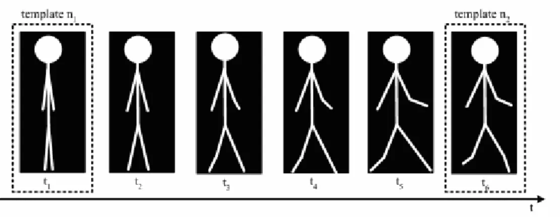
Fig. 3.5 One image frame is selected as template with an interval ... 26

Fig. 3.6 Common states of two different activites... 28

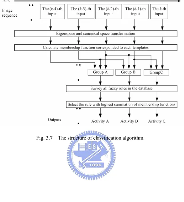
Fig. 3.7 The structure of classification algorithm...34

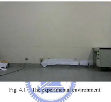
Fig. 4.1 The experimental environment.. ... 35

Fig. 4.2 Various images of our models. ... 36

Fig. 4.3 Background image. (a) Background image in the H components, (b) Background image in the S components. (c) Background image in the V components.. ... 37

Fig. 4.4 H, S, and V variations versus frame index of background video frame 1 to frame 300. (a) H at (10, 10), (b) H at (120, 160), (c) S at (10, 10), (d) S at (10, 10), (e) V at (10, 10), (f) V at (10, 10).. ... 38

(10)

k

1.0 k

Fig. 4.6 An example of foreground extraction at different thresholds.(a) An image frame with subject’s clothing color different from the background, (b)－(f) foreground detected images, (b)

V V = , (c) kV =1.1, (d) kV =1.2, (e) kV =1.3, and (f) k =1.4... 41 k 1.0 k V

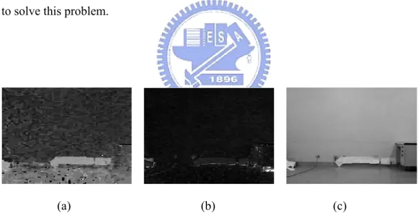
Fig. 4.7 An example of foreground region extraction at different threshold.(a) An image frame with subject’s clothing color similar to the background, (b)－(f) foreground detected images, (b)

V

V = , (c) kV =1.1, (d) kV =1.2, (e) kV =1.3,

and (f) kV =1.4... 42

Fig. 4.8 The example of the shadow detection. ... 43

Fig. 4.9 Foreground detection without and with color compensation. (a)－(f) is the input images, (a1)－(f1) the segmented foreground images, without color compensation, (a2)－(f2) the segmented foreground images with color compensation. ... 45

Fig. 4.10 Some “essential templates of posture,” model A. ... 47

Fig. 4.11 Corresponding “essential templates of posture” of Fig. 4.10, model B. ... 48

(11)

List of Tables

TABLE I COMPARISON RESULT OF THE PIXEL ACCURACY RATE... 46

TABLE II SOME OF THE OBTAINED FUZZY RULE BASE... 50

TABLE III THE FRAME NUMBER OF EACH ACTIVITY IN GROUP AMODELS... 52

TABLE IV THE RECOGNITION RATE OF EACH ACTIVITY IN GROUP AMODELS... 52

TABLE V THE RECOGNITION RATE WITH THE MODEL WEARING YELLOW CLOTHING... 53

Table VI THE RECOGNITION RATEWITH THE MODEL WEARING LIGHT BLUE CLOTHING.. 54

(12)

Chapter 1 Introduction

1.1 Motivation

Human activity recognition from video streams has many applications such as home care system, human-machine interface, and automatic surveillance, etc. However, there is no rigid syntax and well-defined structure in human action recognition system; therefore, it makes human activity recognition a very challenging task.

Several human activity recognition methods have been proposed in the past few years. Yamato et al. [1] turn image frames into a symbol sequence and use HMM to recognize human action. Bobick and Davis [2] recognize human activities by comparing motion-energy and motion-history of template images with temporal images. Cohen and Li [3] use a view-independent 3-D shape description for classifying and identifying human activity using SVMs. There have been some significant projects on detecting, tracking people and recognizing their activities. W4 [4] is one of them. W4 can detect people (single person or people in group) by adopting an adaptive background model and identify the activities by finding the body parts on the silhouette boundary.

The objective of this thesis is to provide a human-like system to auto-surveillance and to track people and identify their activities. This system can tell where the foreground subject is in an image, and what the subject is doing.

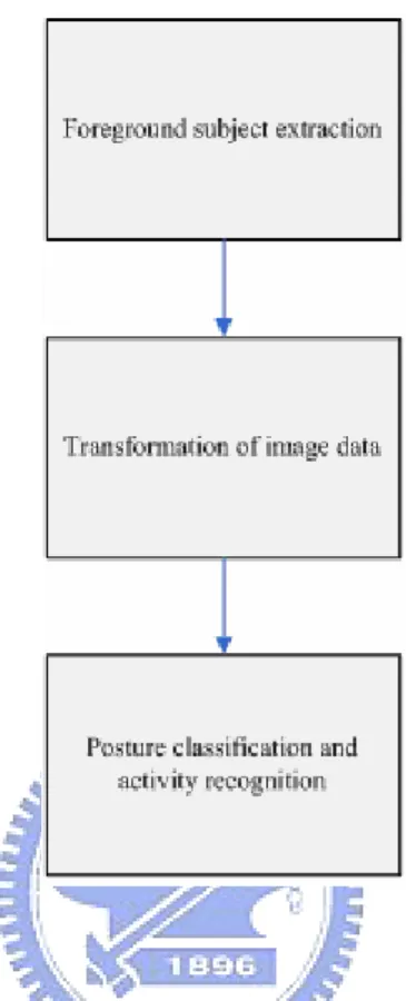
The system flowchart is illustrated in Fig. 1.1 Our system can be separated into three components. The first component is foreground subject extraction. The second component is the transformation of image data in a space smaller and easier for

(13)

posture recognition. The third component is the posture classification of an image frame and activity recognition using frame sequences.

Fig. 1.1 The flowchart of our human activity recognition system.

1.2 Foreground subject extraction

Foreground subject extraction is an important step of the vision-based human activity recognition system. Many authors have developed methods of detecting people in images. Park and Aggarwal subtracted foreground pixels from background by computing Mahalanobis distance in each pixel in the HSV color model [5]. Leung and Yang built a human body outline labeling system [6]. Jabri and Duric [7] used color and edge information to improve the quality and reliability of the results. They all try to find out the real poses a human did by human body outline or by silhouettes.

(14)

Background subtraction is widely used for detecting moving objects from image frames of static cameras. Most of this work has been based on background subtraction using color or luminance information. In these approaches, difference between the coming frame and the background image is performed to detect foreground objects. If we only use the luminance information to do background subtraction, we cannot detect a foreground pixel correctly when it is similar to the background pixel. To make fully use of the spectrum of a pixel, it is imperative to do the segmentation in the color domain. To the end, foreground subject extraction is done in the HSV color space. We can have both the luminance information and the chromatic information in the background subtraction task.

Background subtraction is extremely sensitive to dynamic scene changes due to illumination change. In order to solve the effect of varying luminance conditions, we develop a method which is robust to the illumination changes. The method utilizes frame ratio rather than frame difference in luminance component.

Furthermore, the moving cast shadows mostly exhibit a challenge for accurate foreground subject detection. A lot of attempts have been developed to tackle the shadow suppression [8] [13]encountered in background subtraction. Horprasert et al. [8] and Cucchiara et al. [9] utilized the rationale that shadows have similar chromaticity, but lower brightness than the background model. Under the proposed frame work in the HSV color space, we can effectively identify the shadow existent in our detected foreground subject.

−

After building a background model, we can extract foreground subjects from video frames by subtracting each pixel value of background model from that of current image frame. The resulting image is converted to a binary one by setting a threshold. The binary image mainly contains foreground subjects with only little noise. Therefore, we can set a threshold in the histogram of the binary image to extract a

(15)

rectangle image, which is a good representation resemble shape of a person, of the target subject. The rectangle image is normalized to a uniform benchmark .

1.3 Eigenspace and Canonical Space Transformation

In most video and image processing, the size of frame is usually very large and it usually has some redundancy. The redundancy possesses no information of an image. Hence, some space transformations are introduced to reduce redundancy of an image by reducing the data size of the image. The first step of redundancy reduction often transforms an image from spatiotemporal space to another data space. The transformation can use fewer dimensions to approximate the original image. There are many well-known transformation methods such as Fourier Transformation, Wavelet Transformation, Principal Component Analysis and so on. Our transformation method combines eigenspace transformation and canonical space transformation which are described as follows.

Eigenspace transformation (EST), based on Principal Component Analysis, has been demonstrated to be a potent scheme used widely as shown below: automatic face recognition proposed in [14], [15]; gait analysis proposed in [16]; and action recognition proposed in [17]. The subsequent transformation, Canonical space transformation (CST) based on Canonical Analysis, is mainly to optimize the class separability and improve the classification performance. Unfortunately, CST approach needs high computation efforts when the image is large. Therefore, we combine EST and CST in order to improve the classification performance and reduce the dimension as well. Thus each image can be projected from a high-dimensional spatiotemporal space to a low-dimensional canonical space. In this new space the recognition of

(16)

human activities becomes much simpler and easier.

1.4 Image frame classification and activity recognition

In this thesis each in a video segmentation, images are transformed into an image feature vector by extracting features from images. We utilize eigenspace and canonical space transformation used to extract image features. If we only adopt the shape-based features to recognize an activity, many activities remain unidentified since the temporal information is discarded. Hence, we group three consecutive image feature vectors from three contiguous, but down-sampled images. Consequently, the time-sequential images are converted to a posture sequence by using these three feature vectors. The posture sequence is dignified by the index number of the posture template. In the learning phase, we build a transition model in terms of three consecutive posture sequences which are the category symbols of the posture template. For human action recognition, the model which best matches the observed posture sequence is chosen as the recognized action category.

The most famous method to model transition model of time-sequential data is Hidden Markov Models (HMMs). Hidden Markov Models can deal with time-sequential data and can provide time-scale invariability for recognition. The basic concept of Hidden Markov Models is described in [18]. Hidden Markov Models have been successfully used for speech recognition because of their capability of recognizing spoken words independent of their duration [18]−[20]. Hidden Markov Models also have been used in hand gestures recognition [21] and activity recognition [1]. The price paid for the efficiency in this case is that we have to collect a great amount of data and a lot of time is required to estimate the corresponding parameters

(17)

in HMMs.

After transforming image frames to eigenspace and canonical space domain, some data information have been omitted. By using fuzzy rule-base techniques, the activity analysis task is tolerant to uncertainty, ambiguity and irregularity. Relevant articles using the fuzzy theory are described as follows. Wang and Mendel [22] proposed that fuzzy rules to be generated by learning from examples. Su [23] presented a fuzzy rule-based approach to spatio-temporal hand gesture recognition. He employed a powerful method based on hyperrectangular composite neural networks (HRCNNs) for selecting templates.

In our system, we propose a fuzzy rule-base approach for human activity recognition. Each activity is represented in the form of crisp IF-THEN rules, extracted from the posture sequences of the training data. Each crisp IF-THEN rule is then fuzzified by employing an innovative membership function in order to represent the degree indicating the similarity between a pattern and the corresponding antecedent part in the training data. When an unknown activity is to be classified, sampled image of the unknown activity is tested by each fuzzy rule. The accumulated similarity measure associated with these three consecutive postures is to match the posture sequence representing activity model of the training database, and the unknown activity is classified to the activity yielding the highest accumulative similarity.

1.5 Thesis outlines

The thesis is organized as follows. Before introducing the technique of our human activity recognition system, the basic concepts concerning the HSV color space, eigenspace transform, and canonical space transform are introduced in

(18)

Chapter2. In this chapter, we introduce the HSV color space and discuss the process of how to transform a high dimensional image to eigenspace and canonical space. Chapter 3 describes our human activity recognition system in detail. In Chapter 4, the experiment results of our recognition system are shown. At last, we conclude this thesis with a discussion in Chapter 5.

(19)

Chapter 2 BASIC CONCEPT

In this chapter, we briefly explain the basic concepts of eigenspace and canonical space transform. Then HSV color space concept is introduced.

2.1 Fundamentals of Eigenspace and Canonical Space

Transform

In video and image processing, the dimensions of image data are often extremely large. There are many well-known transformation methods to reduce the size of data such as Fourier transformation, wavelet, principal component analysis (PCA), eigenspace transformation (EST) and so on. However, PCA based on the global covariance matrix of the full set of image data is not sensitive to the class structure existent in the data. In order to increase the discriminatory power of various activity features, Etemad and Chellappa [24] used linear discriminant analysis (LDA), also called canonical analysis (CA), which can be used to optimize the class separability of different activity classes and improve the classification performance. The features are obtained by maximizing between-class and minimizing within-class variations. Here we call this approach canonical space transformation (CST). Combining EST with CST, our approach reduces the data dimensionality and optimizes the class separability among classes.

Image data in high-dimensional space are converted to low-dimensional eigenspace using PCA. The obtained vector thus is futher projected to a smaller canonical space using CST. Action Recognition is accomplished in the canonical space.

(20)

Assume that there are c classes to be learned. Each class represents a specific posture, which assumes of testers various forms existing in the training image data.

is the j-th image in class i, and N i,j

x′ i is the number of images in the i-th class. The

total number of images in training set isNT = N1+N2+L+Nc. This training set can be written as

[

x1′,1 ,L ,x′1,N1 ,L ,x′2,1 ,L ,x′c,Nc

]

(1) where each x′i,j is an image.

At first, the intensity of each sample image is normalized by

. , , , j i j i j i x x x ′ ′ =

(2) Then we can get the mean pixel value for training image as

1 . 1 1 , x

∑∑

= = = c i N j j i T i N x m

(3) The training set can be rewritten as an n×NT matrix X. And each image forms a column of X, that is j i, x

[

x1,1 mx , ,x1, 1 mx , ,x , mx

]

. X= − L N − L cNc − (4)

(21)

2.1.1 Eigenspace Transformation (EST)

Basically EST is widely used to reduce the dimensionality of an input space by mapping the data from a correlated high-dimensional space to an uncorrelated low-dimensional space while maintaining the minimum mean-square error to avoid information loss. EST uses the eigenvalues and eigenvectors generated by the data covariance matrix to retain the original data coordinates along the directions of maximal variance sequentially.

If the rank of the matrix XXT is K, then K nonzero eigenvalues of XXT, λ1, λ2, L,λK, and their associated eigenvectors, , satisfy the fundamental relationship K e e e1 , 2 ,L ,

λi ei =Rei, i=1,2, L,K

(5)

where _R₌_XXT_{and R is a square, symmetric matrix. In order to solve Eq. (5), we}

need to calculate the eigenvalues and eigenvectors of the n× matrix n . But

the dimensionality of is the image size, it is usually too large to be computed easily. Based on singular value decomposition, we can get the eigenvalues and eigenvectors by computing the matrix

T XX T XX R~ instead, that is

data matrix

(6) T _: = R X X% X

in which the matrix sizes of R~ are NT×NT which is much smaller than of R. Still matrix

n n×

R~ has K nonzero eigenvalues K

~ , , ~ , ~ _λ _λ λ1 2 _L and K associated

(22)

( )

⎪⎩ ⎪ ⎨ ⎧ λ = λ = λ − i i i i i e X e ~ ~ ~ 2 1

i = 1 , 2,L,K

(7)

These K eigenvectors are used as an orthogonal basis to span a new vector space. Each image can be projected to a point in this K-dimensional space. Based on the theory of PCA, each image can be approximated by taking only the largest eigenvalues λ₁ ≥ λ₂ ≥_L≥ λ_k , k ≤K , and their associated eigenvectors

. This partial set of k eigenvectors spans an eigenspace in which are the points that are the projections of the original images by the equation

k e e e1 , 2 ,L , yi,j j , i x (8)

[

]

T , , , , 1 2 , 1, 2,..., ; 1, 2,..., i j = k i j i= c j c y e e _L e x = N

]

We called this matrix

[

the eigenspace transformation matrix. After this transformation, each image can be approximated by the linear combination of these k eigenvectors and is a one-dimensional vector with k elements which are their associated coefficients.

T 2 1,e , ,ek e _L j i, x j i, y

2.1.2 Canonical Space Transformation (CST)

Based on canonical analysis in [25], we suppose that

{

φ1,φ2,L,φc

}

represents the classes of transformed vectors by eigenspace transformation and is the j-th vector in class i. The mean vector of entire set can be written as

j i, y

, 1 1, 2, , ; 1, 2, , y i j i j T i c j N =

∑∑

= = m y K K Ni

(9)

(23)

1 . Φ ,

∑

∈ = i i,j j i i i N y y m

(10) Let St denote the total scatter matrix, Sw denote the within-class matrix and Sb

denote the between-class matrix, then

(

)(

)

(

)(

)

(

)(

)

∑

∑ ∑

∑∑

= = ∈ = = − − = − − = − − = c i y i y i i T c i i j i i j i T c i N j y j i y j i T N N N N i j i i 1 T 1 φ T , , 1 1 T , , 1 1 1 , m m m m S m y m y S m y m y S y b w t

where Sw represents the mean of within-class vectors distance and Sb represents the

mean of between-class distance vectors distance. The objective is to minimize Sw and

maximize Sb simultaneously, which is known as the generalized Fisher linear

discriminant function and is given by

( )

_T . T W S W W S W W J w b =

(11) The ratio of variances in the new space is maximized by the selection of feature transformation W if

=0. ∂ ∂ W J

(12)

Suppose that W* is the optimal solution where the column vector is a generated eigenvector corresponding to the i-th largest eigenvalues

* i w

i

λ . According to the theory presented in [25], we can solve Eq. (12) as follows

* _.

(13) i =λi i

S wb S ww *

(24)

After solving (11), we will obtain c–1 nonzero eigenvalues and their corresponding eigenvectors that create another orthogonal basis and span a (c–1)-dimensional canonical space. By using these bases, each point in eigenspace can be projected to another point in canonical space by

[

v1,v2,L,vc

]

zi,j =

[

v1,v2,L,vc−1

]

Tyi,j

(14) where zi,j represents the new point and the orthogonal basis

[

v1,v2,L,vc−1

]

T is

called the canonical space transformation matrix. By merging equation (8) and (14), each image can be projected into a point in the new (c－1)-dimensional space by

(25)

2.2 The HSV color space

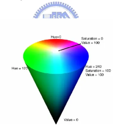
The HSV (hue, saturation and value) color space corresponds closely to the human perception of color. Conceptually, the HSV color space is a cone. Viewed from the circular side of the cone, the hues are represented by the angle of each color in the cone relative to the 0o line, which is traditionally assigned to be red. The saturation is represent as the distance from the center of the circle. Highly saturation color are on the outer edge of the cone, whereas gray tones (which have no saturation) are at the very center. The brightness is determined by the colors vertical position in the cone. At the point end of the cone, there is no brightness, so all colors are blacks. At the fat end of the cone are the brightness colors.

Fig. 2.1 The HSV Cone

(26)

brightness. Therefore, the hue is not affected by change of the illumination brightness and direction. Although hue is the most useful attribute, there are three problems in using hue attribute for color segmentation: (1) hue is meaningless when the intensity value is very low; (2) hue is unstable when the saturation is very low; and (3) saturation is meaningless when the intensity value is very low [11]. Accordingly, Ohba et al. [26] use three criteria (intensity value, saturation, and hue) to obtain the hue value reliably.

z Intensity Threshold Value:

If V <Vt, then H =0, where , V Vt, and Hare an intensity value, the intensity threshold value, and a hue value, respectively. If measured color is not bright enough, the color is discarded. Then, the hue value is set to a predetermined value, i.e., 0.

z Saturation Threshold Value:

If S<S_t, then H =0, where S, St, and Hare an saturation value, the saturation threshold value, and a hue value, respectively. Using this equation, measured color close to gray is discarded in the image.

z Hue Threshold Value:

If H < ΔP_t or H−2π < Δ , then P_t H = . The range of hue value is 0

from 0 to 2π , and it has discontinuity at 0 and 2π . We use the phase threshold value ΔPt to avoid the discontinuity effect.

(27)

Chapter 3 Human Activity Recognition System

3.1 Object extraction

3.1.1 The intensity of the image

We assume the intensity of the image captured by a camera can be described as

( , ) ( , ) ( , ),

i i i

I x y =S x y r x y (16)

where Ii is the intensity of the image, Si is the spatial distribution of source

illumination, ri is the distribution of scene reflectance, (x,y) is the location of a pixel

in the image, and i is the image sequence index. Now we can compare the difference caused by illumination change between frame difference and frame ratio. If we hold the camera still with no foreground subjects pass by, the reflectance of this background should be the same at any time. That is,

(

,

) (

,

)

i

r x y =r x y . (17)

Although the reflectance is not changed, the effect of illumination is still going on. The frame difference and frame ratio between two consecutive frames can respectively be written as

( )

( ) ( )

( )

(

)

( )

1 1 1 , , , , , , , , , , d d d d i i i i d d i i I x y I x y S x y r x y S x y r x y S x y S x y r x y − − − − = − = − (18)

(28)

(

)

(

)

(

) (

)

(

)

(

)

(

)

(

)

(

)

1 1 1 1 log log , , , , log , log , log , , i i r r i i r i r i r r i i I x y S x y r x y S x y S x y S x y S x y − − − − = ⎜ ⎟ ⎜ ⎟ ⎜ ⎟ ⎜ ⎟ ⎝ ⎠ ⎝ ⎠ ⎛ ⎞ = ⎜_⎜ ⎟_⎟ ⎝ ⎠ = − , , , r r I x y S x y r x y ⎛ ⎞ ⎛ ⎞ (19)

where Id_{is the intensity of scene captured by camera of frame difference, S}d_{is the}

spatial distribution of source illumination of frame difference, and Ir_{and S}r_{is of}

frame ratio. Comparing Eqs. (18) and (19), we can find that the problems cause by reflectance still remains in the frame difference approach; nevertheless, the influence of reflectance is eliminated in the frame ratio approach.

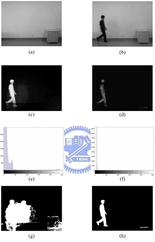
Fig.3.1shows a comparison between frame ratio and frame difference. Fig.3.1(a) is a background image and Fig. 3.1(b) is an image frame with a human. By using frame difference and frame ratio approach, we obtain Fig. 3.1(c) and Fig. 3.1(d), respectively. Gray level of the resulting images distributed from 0 to 255. Fig. 3.1(e) is the histogram of Fig. 3.1(c) and Fig. 3.1(f) is the histogram of Fig. 3.1(d). Comparing the histograms of Fig. 3.1(d) and Fig. 3.1(e), we find out that there was less noise in the region of low gray level by using frame ratio method. The Fig. 3.1(g) and Fig. 3.1(h) are the binary image of extraction images which simply took a threshold value 15 at gray level against Fig. 3.1(c) and Fig. 3.1(d).

(29)

(a) (b)

(c) (d)

(e) (f)

(g) (h)

Fig. 3.1 The comparison between frame ratio and frame difference. (a) Background image, (b) image frame with a human, (c) frame difference, (d) frame ratio, (e) histogram of frame difference, (f) histogram of frame ratio, (g) foreground pixels of frame difference after simply taking a threshold, and (h) foreground pixels of frame ratio after simply taking a threshold

(30)

3.1.2 Background model

If we only use the luminance component to do background subtraction, we cannot detect reliably those foreground pixel whose luminance component close to background pixel. In order to solve this problem, we build our background model in the HSV color space. The HSV color space corresponds closely to the human perception of color. We can have the luminance information and the chromatic information simultaneously. Hue is unreliable in some condition, so we use the three criteria (intensity value, saturation, and hue) described in Chapter 2 to obtain the hue value reliably.

In the previous section, we have seen the advantage of using frame ratio approach to counter the luminance change. Hence, we propose to utilize the frame ratio to build the background model in the luminance component. We build our

background model with the minimum value ( ) and

maximum value ([ ) in each HSV domain. Besides, we

also record the inter-frame ratio in the brightness information and the inter-frame different in the chromatic information.

[ H( , ), S( , ), V( , )]

n x y n x y n x y

( , ), ( , ), ( , )]

H S V

m x y m x y m x y

We need a background video, without any moving objects, for background model training. Suppose the observed image frame sequence contains N consecutive images. H

(

,

i

)

I x y be the pixel’s hue value at

( )

x,y of the i-th image frame.

(

, S

i

)

I x y be the pixel’s saturation value at

( )

x,y of the i-th image frame.

(

, V

i

)

I x y be the pixel’s brightness value at

( )

x,y of the i-th image frame. The

(31)

( )

{

}

( )

{

}

( )

{

1

}

max , , , min , , max , , H H i i H H i i H H H i i i I x y m x y n x y I x y d x y I x y I₋ x y ⎡ ⎤ ⎡ ⎤ ⎢ ⎥ ⎢ ⎥ ⎢₌ ⎥ ⎢ ⎥ ⎢ ⎥ ⎢ ⎥ ⎢ ⎥ ⎣ ⎦ _⎢ ₋ _⎥ ⎣ ⎦ (20)

( )

{

}

( )

{

}

( )

{

1

}

max , , , min , , max , , S S _i i S S i i S S S i i i I x y m x y n x y I x y d x y I x y I₋ x y ⎡ ⎤ ⎡ ⎤ ⎢ ⎥ ⎢ ⎥ ⎢₌ ⎥ ⎢ ⎥ ⎢ ⎥ ⎢ ⎥ ⎢ ⎥ ⎣ ⎦ _⎢ ₋ _⎥ ⎣ ⎦ (21)

( )

{

}

( )

{

}

( )

{

}

( )

{

}

( )

{

}

( )

{

}

1 1 1 max , min , if , , 1 , _max _, _, , max , , min , otherwise max , , V i i V V i i i V V V i i i V V V i i V i i V V i i i I x y I x y I x y I x y m x y _I _{x y} _I _{x y} n x y I x y d x y I x y I x y I x y − − − ⎧ ⎡ ⎤ ⎪ ⎢ ⎥ ⎪ ⎢ ⎥ _≥ ⎪ ⎢ ⎥ ⎪ ⎢ ⎥ ⎡ ⎤ ⎪ ⎢ ⎥ ⎢ ⎥ ⎪ ⎣_{= ⎨} ⎦ ⎢ ⎥ _⎡ _⎤ ⎪ ⎢ ⎥ _⎢ _⎥ ⎣ _{⎦ ⎪} ⎢ ⎥ ⎪ ⎢ ⎥ ⎪ ⎢ ⎥ ⎪ ⎢ ⎥ ⎪ ⎣ ⎦ ⎩ V i (22) where i=1, 2,...,N.

3.1.3 Foreground subject extraction and shadow detection

Fig.3.2 shows the framework we apply to foreground subject extraction. Our framework of foreground subject extraction is composed of four components. The first component is foreground subject extraction by luminance. The second component is the shadow suppression. The third component is the object segmentation. And the finally component is the color compensation to recover the foreground pixels wrongly classified to the background due to their high luminance

(32)

similarly.

Fig.3.2 The framework we apply to foreground subject extraction

A. Foreground subject detection by luminance

Foreground objects can be segmented from every frame of the video stream. Each pixel of the video frame is classified to either a background or a foreground pixel by the difference between the background model and a captured image frame. We utilize the maximum luminance V

(

,

)

(33)

maximum inter-frame luminance ratio V

(

,

)

d x y of the training background model

to segment the foreground pixel by

0, if ( , ) ( , ) ( , ) or ( , ) ( , ) ( , ) ( , ) 255, otherwise V V V i V V V V i V I x y m x y k d x y I x y n x y k d x y B x y ⎧ < ⎪ < ⎪ = ⎨ ⎪ ⎪⎩ (23) where V

(

,

)

i

I x y is the intensity of a pixel which is located at

( )

x,y , is

the gray level of a pixel in a binary image, and is a threshold, determined by light sufficiency of the scene. The value of is normally set to 1.3 for normal

light condition, and will be reduced for in-sufficient light condition and increased otherwise.

(

x y B ,

)

V k V k V k B. Shadow suppression

The pixels of the moving cast shadows are easily detected as the foreground pixel in normal condition. Because the shadow pixels and the object pixels share two important visual features: motion model and detectability. For this reason, the moving shadows cause object merging and object shape distortion. Horprasert et al. [8] and Cucchiara et al. [9] utilize the rationale that shadows have similar chromaticity, but lower brightness than the background model. Hence, we can detect the shadow from foreground subject in the HSV color space. We analyze only points belonging to possible moving object that are detected in step A. We define a shadow mask S for each ( , )x y point as follows:

(34)

shadow, if ( , ) ( , ) 0 and ( , ) ( , ) (x,y) ( , ) _and _{( , )} _{( , )} _(x,y) object, V V i H H H i H S S S i S I x y n x y I x y m x y k d S x y _I _{x y} _m _{x y} _{k d} − < − < = ₋ _< otherwise ⎧ ⎪ ⎪ ⎪ ⎨ ⎪ ⎪ ⎪ ⎩ (24) where H( , ) i I x y ,IiS( , )x y , and

(

,

)

V i

I x y are respectively the HSV channel of a

pixel located at , and is the shadow mask to class the pixel in the moving cast shadow. Values and

(

x,y

)

S x y

(

,

)

S

k kH are selected threshold values used to

measure the similarities of the hue and saturation between the background image and the current observed image. We can utilize the shadow mask to change the shadow pixels into background in

( , ) S x y ( , )

B x y .

C. Object segmentation

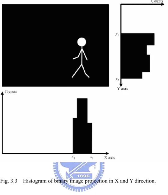
According to the binary image B segmented by above, we extract the region of foreground object to minimize the image size. Foreground region extraction can be accomplished by simply introducing a threshold on the histograms in X and Y direction. Fig. 3.3 shows an example of foreground region extraction. We utilize the binary image and project it to X and Y directions. The interested section has higher counts in the histogram. We obtain the boundary coordinates x1, x2 of X axis and y1,

y2 of Y axis from the projection histogram. We can use these boundary coordinates

as the corner of a rectangle to extract foreground region (Bs). Fig. 3.4 is the

(35)

Fig. 3.3 Histogram of binary image projection in X and Y direction.

(36)

D. Color compensation

Some colors such as yellow, pink, and light blue have similar luminance value. If we only use the luminance component to do background subtraction, we cannot detect foreground pixel correctly when its luminance is similar to that of a background pixel. In order to improve detectability, background subtraction is computed by taking into account not only a point’s luminance, but also its chromaticity. We want to use the chromaticity to enhance the accuracy of the foreground object. We only analyze the region Bs obtained in subsection C above.

Based on the amount of the chromaticity change, we reanalyze its background in

s

B to be changed to a foreground of object, by

255, if ( , ) ( , ) (x,y) or ( , ) ( , ) (x,y) ( , ) 0, otherwise S S S i S H H H i H f I x y m x y k d I x y m x y k d B x y ⎧ − > ⎪ ⎪ ₋ _> = ⎨ ⎪ ⎪ ⎩ (25) where H( , ) i

I x y andIiS( , )x y are respectively the hue and saturation components of a

pixel at

( )

x,y , kS and kH are selected threshold values. B is the final f

(37)

3.2 Activity template selection

A human body is a rigid body, thus has its natural frequency; namely, it has restriction on action speed when doing some specific actions. Because cameras usually capture image frames in a high frequency, there are few differences between two postural image frames in a short interval. Therefore, we select some key frames from a sequence to represent an activity. In our approach, we select one image frame, called as the essential template image, with a fixed interval instead of each image. An example is shown in Fig. 3.5. After determining the templates, each activity is represented by several essential templates.

Fig. 3.5 One image frame is selected as template with an interval.

These essential templates are transformed to a new space by eigenspace transformation (EST) and canonical space transformation (CST). The approximation can decrease data dimension, but it would also lose slight information of image with few differences. However, two similar image frames will converge to two near points after eigenspace and canonical space transformation. The images of similar postures done by difference people also barely converge to one point. Consequently, we select only essential templates rather than use all sequences for human activity

(38)

recognition.

As described in Chapter 2, each image frame is transformed to a (c–1)-dimensional vector by EST and CST methods. Assume that there are n training models and c clusters in the system. Therefore, we have Nt templates, where Nt is

equal to n multiplied by c. Let be a vector of template image of the j-th

training model and the i-th category and be the transformed vector of .

is computed by j i, g j i, t gi,j j i, t , , , 1, 2, , ; 1, 2, , i j = × i j i= c j= t H g _L _{L (26)}n

where H denote the transformation matrix combing EST and CST and n is the total number of posture images in the i-th cluster. is a (c–1)-dimensional vector and

each dimension is supposed to be independent. Hence, is rewritten as j i, t j i, t T 1 2 1 , , , , , , , . c i j ti j ti j ti j − ⎡ ⎤ = ⎣ ⎦ t _L (27)

The transformation of each training model’s templates is treated as a mean vector. That is,

,

i j = i j

μ t_, (28)

where i is the number of template categories. The standard deviation vector of the

(39)

(

)

1 1 1 2 , , − − =

∑∑

= = t c j n i m j i m j i m N t μ σ (29) where m=1 ,2,_K ,c−1.

3.3 Construction of fuzzy rules form video stream

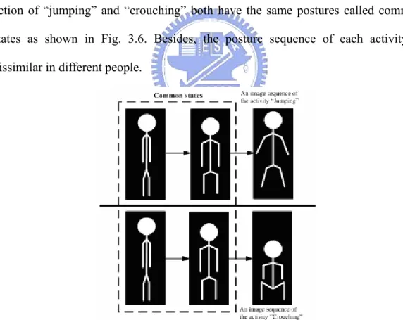
Transitional relationships of postures in a temporal sequence are important information for human activity classification. If we only utilize one image frame to classify the action, classification result may be failed easily because human’s actions may have similar postures in two different activity sequences. For example, the action of “jumping” and “crouching” both have the same postures called common states as shown in Fig. 3.6. Besides, the posture sequence of each activity is dissimilar in different people.

Fig. 3.6 Common states of two different activites.

(40)

information for recognition but also is tolerant to variations of different people. We use the fuzzy rule-base approach to design our system. The fuzzy rule-base approach also has been proposed in gesture recognition in [23]; it has ability to absorb data difference by learning.

We use the membership function to represent the feature’s possibility of each cluster. Many types of membership functions, e.g., bell-shaped, triangular, and trapezoid ones, are frequently used in a fuzzy system. We choose the Gaussian type membership function to represent the features because the Gaussian type membership function can reflect the similarity via the first order and second order statistics of clusters and is differentiable.

Firstly, when the k-th training image frame xk is inputted, the feature vector ak

is extracted by

ak =Hxk. (30)

As the same as ti,j in Eq.(27), ak can be rewritten as

[

, , , 1 T. (31) , 2 1 − = c j i k k k a a L a a

]

If we assume the dimensions of the feature vectors are independent, a local measure of similarity between the training vector and each template vectors can be computed. Let Σ denote the covariance matrix of all essential template vectors and

(41)

( )

(

)

, T 1 1 1 2 2 2 , 2 ( | ) 1 1 exp 2 2 1 1

arg max exp

2 2 i k k i k k c k i j j r M C a π μ σ πσ − − = ⎡ ⎤ = _⎢− _⎥ ⎣ ⎦ ⎧ ⎡ ₋ ⎤⎫ ⎪ _⎢ _⎥⎪ = _⎨ _⎢− _⎥_⎬ ⎪ _⎢_⎣ _⎥_⎦⎪ ⎩ ⎭ a a Σ a Σ (32)

where j is the training model number. denotes the grade of membership function in category i of the k-th image frame. Besides, we can obtain which category each image belongs to by

k i r, , i arg max k i p = r_k (33)

The membership function describes the probability of which one it is like most. But it just contains the information of a single image. Hence, we collect three images to form a basis for temporal information. If we use too many images to form a basis, the data may contain too many images of other activity. If we use too few images, it may not have enough timing information to represent an activity.

Assume we have c linguistic labels, each linguistic label represent a category of essential template. Each image frame can be represented by one of these c linguistic labels. In our approach, we combine three contiguous images to a group ( ,I₁ I I₂, )₃

]

, ]

a a a

. The transformation of the image group can form a feature vector .There are c

1, 2 3

[a a a,

3_{combinations of the feature vector. Each combination represents the possible}

transition states of the three images. We use Eqs. (32) and (33) to class each image frame. Hence, we can represent the feature vector ([ , ) by linguistic label sequence ( ). An image sequence with linguistic label sequence is associated with its output of corresponding activity.

1 2 3

[ , , ]i i i

(42)

As developed by Wang and Mendel [22], fuzzy rules can be generated by learning from examples. Such image sequence constitutes an input-output pair to be learned in the fuzzy rule base. In this setting, the generated rules are a series of associations of the form

“IF antecedent conditions hold, THEN consequent conditions hold.”

The number of antecedent conditions equals the number of features. Note that antecedent conditions are connected by “AND.” For example, an image sequence, its transformations of image 1, image 2, image 3 and belonging categories being concatenated as vector format, is given by

[

a11,a12,a13;D1

]

(34)

Suppose that Image 1, Image2 and Image 3 belong to category 1, category 2 and category 3 respectively. Therefore, we assign the image sequences, whose feature vector is [ , , ], to the linguistic labels Posture 1, Posture 2 and Posture 3 respectively. Finally, a rule is produced from the feature-target vector. Hence this image sequence supports the rule of

1 1 a 1 2 a 1 3 a

(43)

Rule 1. IF the activity’s I1 is P1 AND its I2 is P2 AND its I3 is P3, THEN the

activity is D1. (35)

where Ii is Image i and Pj is Posture j.

Our system is able to learn the hidden transition modes of activities from data. This is an advantage of our system and it will also improve the correct rate in classification. For example, the Posture 1 is a posture of activity D1 but D4, the system still learn a sequence with Posture 1 as the activity D4. We regard Posture 1 as a common state of the two activities D1 and D4. Therefore the fuzzy rules induce tolerant to some ambiguous postures of different activities and classify the image sequence to an activity more correctly.

Sometimes conflicting rules may be generated; they have the same image sequence but refer to different activity. Therefore, we have to choose one from the two or more conflicting rules from each qualified cluster. To this end, we choose the rule that is supported by a maximum number of examples. Furthermore, to prune redundant or inefficient fuzzy rules, if the supporting actions of a rule are less than a threshold, the rule is excluded from defining an IF-THEN rule.

3.4 Classification algorithm

After constructing the rule base, we can grade the input image sequence with each fuzzy rule by grade of membership function. Let Σ denote the covariance matrix of all essential template vectors, Ci denote the i-th class of essential templates

and sk denote the image frame transformed by EST and CST. The membership

(44)

(

)

( )

(

)

(

)

(

)

, T 1 1 1 2 2 2 , 2 j M 1 1 exp 2 2 1 1

arg max exp

2 2 i k k i k k c k i j r C s μ μ π μ σ πσ − − = ⎡ ⎤ = _⎢− − − _⎥ ⎣ ⎦ ⎫ ⎡ ₋ ⎤ ⎧ _⎢ _⎥⎪ = _⎨ _⎢− _⎥_⎬ ⎩ _⎢_⎣ _⎥⎪ ⎦⎭ s s Σ s Σ (36)

where j is the training model number. denotes the grade of membership function in category i of the k-th image frame. σ is the standard deviation of all essential templates. These membership functions are just the results of one image frame. We need to collect three images as a group for recognizing an activity. Therefore, we use two more transformed vector of passed image frames, which are called and . These three vectors form a feature vector [ , , ]. We compute the membership functions of the three vectors respectively. The procedures of calculating membership functions of and are the same as the process used for in Eq. (36).

k i r, 2 − k a ak−1 ak−2 ak−1 ak 2 − k a ak−1 k a

In order to calculate the similarity between image sequence and each postural sequence in the training data base, we take out the membership functions , and which are corresponding to the three category of linguistic labels, , and , in the rule and have been calculated by Eq. (36). The summation of , and is the similarity between current image sequence and the postural sequence of this rule. We can obtain the similarity related to all fuzzy rules of training data base in the same manner. The rule, which has the highest value of similarity, is selected and the unknown activity is classified to the activity recorded in this rule. Fig. 3.7 shows the structure of the classification algorithm.

1 , 2 n k r− 2 , 1 n k r− rk,n3 1 Pn Pn2 Pn3 1 , 2 n k r− rk−1 n,2 rk,n3

(45)

(46)

Chapter 4 Experimental Result

In our experiment, we tested our system on videos taken by digital camera. We took the video in our laboratory at the 5th Engineering Building in NCTU campus. The camera has a frame rate of thirty frames per second and image resolution is

pixels. The experimental environment is shown in Fig. 4.1. 320 240×

Fig. 4.1 The experimental environment.

The background is not complex and we equipped a table in the scene. The light source is fluorescent lamps and is stable. Each person performed six actions: “walking from left to right,” “walking from right to left,” “jumping,” “crouching,” “climbing up” and “climb down.” The action “climbing up” is to climb up on the table from the ground. The action “climbing down” is to climb down to the ground from the table.

We test the foreground detection capability and then the action recognition accuracy in two cases depending on the color of clothing worn by action subjects. That the action subject wore the clothing with color different from that of background is first case. And the second case is that the action subject wore the clothing with color similar to that of background. When the color of clothing and

(47)

background are similar in the second case, a moving object, such as human body, may not be segmented easily from image frame. We compare the result in these two cases and the color compensation in our action recognition system demonstrates eminent improvement in the segmentation quality. We classify our model into two groups: Group A has six models in which the subject wears clothing with color different from the background, and Group B has three models in which the subject wears clothing similar to the background. Fig. 4.2 shows our models in the experiment.

(48)

4.1 Background model construction

We built the background model in the HSV color space. The value of H or S or V is between 0 and 255. Figs. 4.3(a), 4.3(b), and 4.3(c) show the background image in the H, S, and V component, respectively. We can find from these three figures that the hue value is relatively unstable when the saturation is close to zero. We make an experiment to test the changes in the HSV components in constructing the background model. Fig. 4.4 represents the H, S, and V variations of two pixels at coordinates ( , )x y = (10, 10) and ( , )x y = (120, 160) during the first 300 frames in

the background video. From Fig. 4.4, we can see that V component is most stable of the background model. H and S components are less stable than V. Hence, we need to solve this problem.

(a) (b) (c)

Fig. 4.3 Background images. (a) Background image in the H component, (b) Background image in the S component, and (c) Background image in the V component.

(49)

(a) (b)

(c) (d)

(e) (f)

Fig. 4.4 H, S, and V variations versus frame index of background video frome frame 1 to frame 300. (a) H at (10, 10), (b) H at (120, 160), (c) S at (10, 10), (d) S at (10, 10), (e) V at (10, 10), and (f) V at (10, 10).

(50)

In Sec. 2.2, we know that hue is unreliable when the color is close to the gray tones. Hence, we use three criteria ( ) to obtain the hue value reliably in building the background model. In our experiment, we set three criteria by

, , t t t V S H 50, 50, and 25 t t t V = S = H =

to make hue value reliably.

Fig. 4.5 shows the background image in the H color components after we use criterion to redefine it. We can find that the hue values in the background image are almost be set to zero. The reason is that our background is simple and the color is similar to the gray tones.

(51)

4.2 Foreground subjects extraction

The V color component is stable and reliable, but it has two drawbacks: the illumination change make it change and the similar color such as yellow, pink, and light blue has the similar value in it. In normal condition, the subjects wear the clothing with the color different from the background, so we can do background subtraction with good performance in the V color component.

In the first step, we use the frame ration in the V color component to get the binary image B x y( , )in Eq. (23) described in Sec. 3.1.3. The value is chosen

by experiments and varies with different trials. Hence, we ran a series of experiments to determine the optimal threshold . Fig. 4.6 shows the binary image

V

k

V

k ( , )

B x y got by different i with subject’s clothing color different from the

background. Fig. 4.7 shows the binary image

V

k

( , )

B x y got by different with

subject’s clothing color similar to the background. Comparing Figs. 4.6 and 4.7, we can find that if the color is different from the background, we can use the threshold value to get a good foreground subject extraction. But we cannot adjust to get a complete and noise-free foreground subject when the clothing color is similar to the background. After the experiment, we set

V k V k kV 1.3 V k = in our system.

(52)

(a) (b)

(c) (d)

(e) (f)

Fig. 4.6 An example of foreground extraction at different kV thresholds.

(a) An image frame with subject’s clothing color different from the background, (b) (f) foreground detected images, (b) − kV =1.0, (c) kV =1.1, (d) , (e)

, and (f) 1.2 V k = 1.3 V k = kV =1.4

(53)

(a) (b)

(c) (d)

(e) (f)

Fig. 4.7 An example of foreground region extraction at different kV threshold. (a) An image frame with subject’s clothing color similar to the background, (b)−(f) foreground detected images, (b) kV =1.0, (c) kV =1.1, (d) kV =1.2, (e) ,

and (f) , 1.3 V k = 1.4 V k =

The influence of shadow makes the foreground subjects distort and influence the recognition result. We use the shadow mask in Eq. (24) described in Sec. 3.1.3 to classify the pixels whether it is a shadow point or not. Fig. 4.8 shows the process result in shadow suppression. Fig. 4.8 (a) and (b) are two input images. Fig. 4.8 (c) and (d) are the foreground subject without shadow detection. The foreground subject

(54)

with shadow detection is shown in Fig. 4.8 (e) and (f).

(a) (b)

(c) (d)

(e) (f)

Fig. 4.8 The example of the shadow detection.

The model in Group B contains three action subjects wear light blue clothing, yellow clothing, and pink clothing, respectively. In the previous experiment, we cannot adjust to get a complete and clean foreground subject in Group B. Hence, we do the color compensation in Eq. (25) described in Sec. 3.1.3. In what follows, the effectiveness of color compensation in obtaining a more accurate foreground is described. In Fig. 4.9, the left column contains input images; the middle column contains the resulting foreground images, without color com-

V

(55)

pensation step; and the right column is the foreground images detected with color compensation step. From the Fig.4.9, we have found that we can get good compensation when the clothing color is light blue and yellow, but cannot obtain good compensation when the clothing color is pink. The reason is that when pink color pixels are transformed from RGB color space to HSV color space, the saturation of pink is lower than the set criterion . Hence, we cannot recover those pixels from background to foreground for such small chromaticity difference in this space.

t

S

(a) (a1) (a2)

(b) (b1) (b2)

(56)

(d) (d1) (d2)

(e) (e1) (e2)

(f) (f1) (f2)

Fig. 4.9. Foreground detection without and with color compensation. (a) (f) is the input images, (a1) (f1) the foreground images, without color compensation, (a2) (f2) the foreground images detected with color compensation.

− −

−

We randomly selected 100 frames from the video sequence of the model with a subject wearing clothing similar to the background color. The “ foreground subject ground truths” of these 100 frames were generated manually. Let A be a detected foreground subject region and B be the corresponding “ground truth.” Then we test the pixel accuracy by the following two metrics. Metric 1 is a measure concerning whole segmented region pixels relative to these pixels in A the same with in B. To this end, we calculate the accuracy rate by

(57)

1

Accuracy rate = s 100%,

total

N

N × (37)

where Ntotal is the pixel number of segmented foreground image, and Ns is the

pixel number that the pixel in A is the same as that in B, i.e., such of true positive and false negative pixels of A relative to B. Metric 2 is adopted from [27] by

2 Accuracy rate A B 100%, A B ∩ = × ∪ (38)

This measure counts the percentage of the mutual positive pixels to expanded positive pixels. Table I shows the accuracy rate in metric 1 and metric 2 of 100 frames, and demonstrates the improvement of color compensation over that without color compensation.

TABLE I

COMPARISON RESULT OF THE PIXEL ACCURACY RATES OVER 100IMAGES

Without color compensation With color compensation

Metric 1 78.81% 89.13%

Metric 2 59.61% 81.23%

4.3 Fuzzy rule construction for action recognition

We construct the template model matrix and the fuzzy rule database with the Group A. We chose six kinds of essential templates for “walking from left to right,” “walking from right to left,” and “climb down,” respectively; five for “climbing up,” three for “crouching” and two for “jumping.” There are total 28 kinds of essential templates, and called 28 classes. The essential template numbers of each activity

(58)

depend on how long it takes. Each essential template is a cluster with five template images which are from five different training person’s and have similar postures. Fig 4.10 and Fig. 4.11 are two examples of some templates of two training model.

Class 3 Class 5 Class 8

(59)

Fig. 4.11 Corresponding “essential templates of posture,” Fig. 4.10, of model B.

The template images are transformed to canonical space by the methods described in Chapter 2. The mean vectors and the standard deviation vectors of all templates were computed by Eq. (29). Each template image of a training model was treated as a center. Hence, there were 140 mean vectors because of five training models and 28 classes of templates. Besides, there were six groups of standard deviation vectors and mean vectors because of six kinds of different training models.

After determining the standard deviation vectors, the corresponding training video frames are inputted. The relationship between each image frame and each template is calculated by using Eq. (32) in Section 3.3. We gathered three images as

HSV色彩空間前景物體抽取及其於人體動作辨識系統應用

國 立 交 通 大 學

電 機 與 控 制 工 程 研 究 所

碩 士 論 文