發展及整合一個以尼摩繞線器為核心的繞線軟體工具

國

立

交

通

大

學

資訊科學與工程研究所

碩

士

論

文

發展及整合一個以尼摩繞線器為核心的繞線軟

體工具

Development and integration of a Gridless Routing Tool Based

on NEMO Detailed Router

研 究 生：徐浩天

指導教授：黃俊龍、李毅郎 教授

發展及整合一個以尼摩繞線器為核心的繞線軟體工具

Development and integration of a Gridless Routing Tool Based on NEMO

Detailed Router

研 究 生：徐浩天 Student：Hao-Tien Hsu

指導教授：黃俊龍、李毅郎 Advisor：Jiun-Long Huang

Yih-Lang Li

國 立 交 通 大 學

資 訊 科 學 與 工 程 研 究 所

碩 士 論 文

Submitted to Institute of Computer Science and Engineering College of Computer Science

National Chiao Tung University in partial Fulfillment of the Requirements

for the Degree of Master

in

Computer Science

August 2007

Hsinchu, Taiwan, Republic of China

發展及整合一個以尼摩繞線器為核心的繞線軟體工具 研究生 : 徐浩天

摘要

Development and integration of a Gridless Routing Tool Based on

NEMO Detailed Router

Student: Hao-Tien Hsu Advisor: Dr. Jiun-Long Huang

Dr. Yih-Lang Li

Institute of Computer Science and Engineering

National Chiao Tung University

Abstract

In modern VLSI designs interconnection deeply affects performance, reliability, and manufacturing cost. Some gridless routing models were proposed to handle variable-width and variable-space routing problems. In a recent work, a gridless detailed router called NEMO, was presented to gain the advantages of the implicit connection graph and tile-based approaches, two gridless routing models.

Based on NEMO, we first enhance and improve its’ structure and output information, and then we combine NEMO and a congestion-driven global router into a routing tool with GUI that provide fundamental display feature such as zoom-in and zoom-out.

Acknowledgment

I am deeply grateful to my advisors, Dr. Jiun-Long Huang and Yih-Lang Li for their continuous guidance, supports, and ardent discussions throughout this implementation work. Especially Dr. Li, his valuable suggestions help me to complete the thesis. Also I express my sincere appreciation to all classmates in my laboratory for their encouragement and help.

This thesis is dedicated to my parents and my families for their patience, love, encouragement and long expectation.

Contents

Abstract (in Chinese) ... I Abstract (in English) ... II Acknowledgment ...III Contents ...IV List of Figures ... V List of Tables...VI Chapter 1 Introduction ...1 Chapter 2 Preliminary ...5

2.1 Routing Model of NEMO ...5

2.2 Routing Feature...7

2.3 Main Concept...9

2.4 Full-chip Routing ... 11

Chapter 3 Implementation issue...12

3.1 Implementation of non-zero width wire model ...12

3.2 Enhancement of path searching and construction...13

3.3 Wire refinement ...16

Chapter 4 Tool integration ...20

4.1 Nets decomposition...20

4.2 Tool design flow...22

Chapter 5 Experiment Results ...24

Chapter 6 Conclusions ...27

List of Figures

1 A layout presented in different graphs………..2

2 Multi-plane routing graph...………...………..6

3 Non-zero wire width model…..………...……….6

4 Multi-layer model…..………...7

5 Entry point………...……….…………...…….8

6 Pseudo pin-to-path routing………...9

7 Example of PMT extraction………...10

8 Routing example with three obstacles...……..……...10

9 Two implementation...……….………...13

10 Center line area in a PMT………..……..………...13

11 Overlap area………...14

12 Estimating cost in tile propagation……...………...15

13 Path construction……….………...16

14 Two cases of space violation………...16

15 A solution of a violation case………...17

16 Apply a solution to other directions………...17

17 A case of space violation and solution……….………..……...18

18 Apply a solution to other directions..………...18

19 A case of space violation and solution……….…….…………...18

20 Separate a steiner tree...………..……...20

21 Separate a steiner tree (cont.)……..……….….…...20

22 Separate a steiner tree (cont.)………..……...20

23 Tool design flow……….….…...21

List of Tables

1 Statistics of ISCAS89 series benchmark circuits...24

2 Comparison of the routing result of ISCAS89 series benchmarks ...25

3 Statistics of Ibm-series Benchmark circuits...25

Chapter 1

Introduction

As very large scale integrated (VLSI) circuits step into the era of deep submicron (DSM) technology and System on Chip (Soc) design methodology, layout optimization issues concerning feature size reduction and design rule variation become more complex and substantial than before. Interconnection design deeply affects performance, reliability, and manufacturing cost, thus interconnection optimization has been well studied these years, such as wire sizing, buffer insertion, double via insertion, etc. For detailed routing, variable-width and variable-space routing request attracts some researcher to get involved in developing gridless routing model and algorithm.

Conventional routing consists of global routing and detailed routing. In global routing stage, the routing region is partitioned into tiles or channels and a global routing path is composed of a series of connected tiles to direct the following detailed router, which identifies precise position and layer of the routing path in each tile. From the viewpoint of routing graph, detailed routers are categorized in two types: grid-based and gridless routers. Their differences mainly reflect on the flexibility of dealing with variable-width and variable-space routing. Grid-based routers search paths on a uniform grid graph. On the contrary, gridless routers search path on a non-uniform grid graph or a non-grid graph, such as a tile-based graph. Compared with grid-based routers, gridless routers are more suitable to complete variable-rule routings.

(a) (b)

(c) (d)

(e) (f)

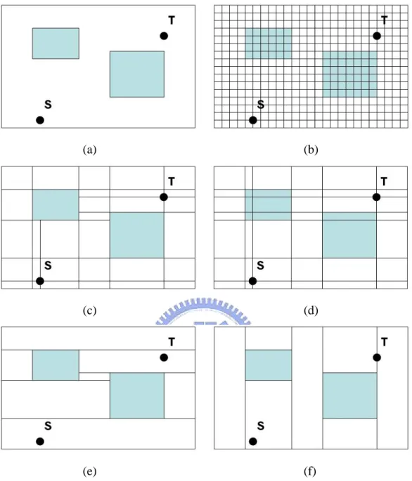
Figure 1 (a) Layout with two obstacles and two terminals; (b) fine uniform grid graph of the layout; (c) connection graph of the layout; (d) implicit connection graph of the layout; (e) maximum horizontally stripped tile plane for the case in (a); (f) maximum vertically stripped tile plane.

Figure 1 display four kinds of routing graphs for gridless routers. Figure 1(a) shows a layout containing two obstacles with two routing terminal S and T; Figure 1 (b) presents the routing graph in uniform fine grid graph model. This model requires substantial runtime and memory usage for a large design. Some approaches for decreasing the complexity of routing graph have been explored in [1][1]~[12]. Among them, the connection graph and tile-based graph are the most widely used approaches. In the work of [10], connection graph is constructed by first extending the boundary of all obstacles until reaching other obstacles or routing boundary (Figure 1(c)). However this approach has expensive cost of representing a connection graph and non-optimal multilayer routing. An implicit presentation for connection graph is presented in [12]. The extension of boundary lines in an implicit connection graph does not halt until reaching the boundaries of routing region (Figure 1 (d)). The final routing graph is produced by integrating the routing graphs of all layers into a routing plane. In an implicit connection graph, a grid point may locate in a blockage; thus we have to decide if it is legal or not when entering a new unvisited grid point. Although the implicit presentation has more grid nodes than that in [10] and has to spent additional time in checking the legality of a move to an unvisited node, optimal multilayer routing, fast query about the legality of a move, and fast construction of a non-uniform grid graph in array data structure are the primary contributions of [12].

The other well-known approach is the tile-based router [2]~[8]. It partitions the total routing region through existing blockages into two tile types, space tiles and block tiles; then corner-stitching data structure [13] is employed to organize all tiles on a tile plane. The routing plane of a horizontal/vertical routing layer is presented in a maximum horizontal/vertical stripped (MHS/MVS) property, where MHS/MVS property is implemented by extending all horizontal/vertical border lines of obstacles until reaching any other obstacle or routing boundaries (Figure 1(e)(f)).

Both the implicit connecting graph and tile-based approaches can find an optimal path in point-to-point routing. The former has the advantages of fast graph construction and query operation; however, the large number of grid points for a big design make fast path searching infeasible. On the contrary, corner-stitching tile planes realize effective path searching for tile-based routers, but require relative large runtime for their construction. In a recent work, a new modified implicit connection graph based router with multi-layer planes, called NEMO [14], was presented to gain the advantages of the implicit connection graph and tile-based approaches. NEMO seeks path like a tile-based router while constructing routing planes like an implicit connection graph based router.

In this thesis, we implement a gridless routing tool combing a congestion-driven global router and NEMO with some improvements and enhancements in NEMO’s structures and output format. This routing tool possesses fundamental GUI features such as zoom in and zoom out.

Chapter 2

Preliminary

In this chapter, we overview NEMO[14] in four parts – routing model, routing feature, main concept, and full-chip routing.

2.1 Routing Model of NEMO

2.1.1 Multi-plane routing graph

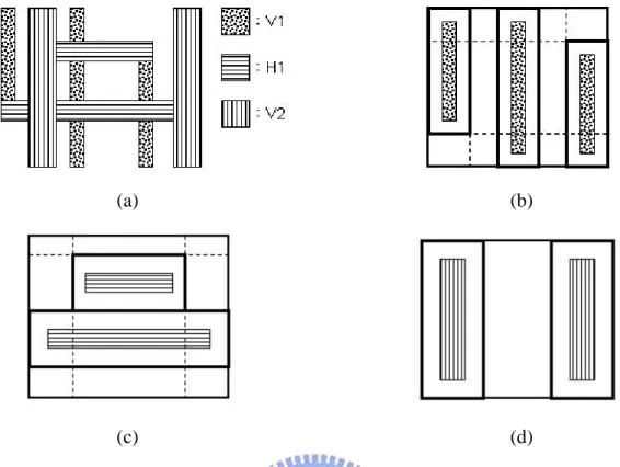
The original implicit connection graph uses two arrays to memorize horizontal and vertical gridlines that are generated by the extending lines of all obstacles on all routing layers. However, the underlying routing graph tends to be too large to fast search path because the border lines of expanded obstacles of different layers probably do not match. NEMO constructs a routing plane for a routing layer to solve this problem. Each plane graph only records the expanded obstacles of its layer. Figure 2(a) presents a 3-layer routing layout; Figure 2(b), (c) and (d) show its associated three routing planes.

2.1.2 Non-zero width wire model

NEMO inserts a contour to every obstacle to prevent from design rule violation. The contour size is ws + ww/2 - vs, where ww is the wire width, ws is the wire space,

and vs is a unit of width. NEMO considers a routing plane as grouped tiles instead of

an array of grid points. In Figure 3, a space tile of width of two times of vs will appear

(a) (b)

(c) (d)

Figure 2 (a) Example of three-layer routing; (b) routing plane for the V1 layer, (c) routing plane for the H1 layer, and (d) routing plane for the V2 layer.

Figure 3 Example of two obstacles separated by a distance of 2×ws+ww. A space tile of width of two times of vs exists between two expanded obstacles for the non-zero width wire model.

2.1.3 Multi-layer model

For layer switching, NEMO builds projection array to store the first tile on adjacent layer to overlap current tile. For example, in Figure 4, Lnx(m) presenting the

m th gridline in n layer in x direction, gridline L2x(2) in projection array points to

gridline L1x(1). Through the projection arrays of x- and y-coordinate, we can simply

calculate all the tiles overlapping current tile in constant time.

2.2 Routing Feature

Because this work focuses on improvement and enhancement of implementation, we introduce some routing feature of NEMO that related our implementation issue in this section.

2.2.1 Minimum cost point

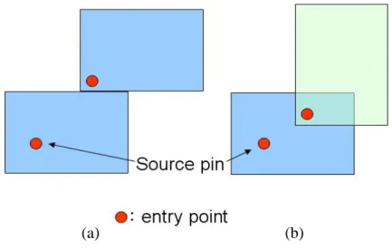
This concept is from the work [6]. When tile propagate every tile records a minimum cost rectangle for path construction. In NEMO we records a point called entry point; every tile searched has an entry point which is on the location most close to last entry point, and source pin is the entry point of the source tile. Figure 5 shows

(a) (b)

Figure 4 (a) New implicit connection graph for two-layer routing plane with gridline notation; (b) the projection array of (a).

tiles and entry points. The main purpose of entry points is that help us estimate approximate cost when tile propagate and NEMO also use it to construct path by connecting entry points.

use pin-to-pin routing to perform pseudo pin-to-path routing. If the ot include two pins, we route this two-pin net with pseu

(a) (b)

2.2.2 Pseudo pin-to-path routing

NEMO

Figure 5 (a) Entry points on two tiles in the same layer ;(b) entry points on two tiles in different layer.

global path of a two-pin net does n

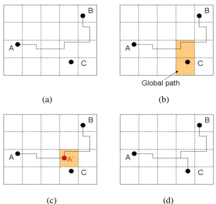
do pin-to-path routing method. This is an example showed in Figure 6. If we have a net with three pins：A, B, and C, and A has already connected with B (Figure 6(a)). Now we want to connect A and C, but the global path only include C (Figure 6(b)). So we search weather a segment of this net is in the terminal of the global path, and set a point A’ on the segment, if there is one (Figure 6(c)). Finally we connect C to A’ instead of connect C to A (Figure 6(d)).

(b) (a)

(c)

2.3 Main Concept

NEMO takes the advantages of the quick and simple graph construction of implicit connection graph model and th

(d)

Figure 6 Pseudo pin-to-path routing (a) A net with three pins A, B, and C,

global path, and mark a point A’ on the segment. (d) Connect C to A’ indeed and A was connected to B. (b) Connect A and C with global path that not include A. (c) Find a segment belong this net in a terminal global cell of the

of connect C to A.

e fast path searching on maximum ripped tile plane.

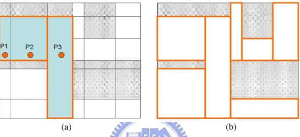
NEMO regards a routing plane as comprising tiles, each of which is identified by its left bottom corner. To behave as a pseudo corner-stitching tile plane, it groups adjacent tiles as a pseudo maximum horizontally or vertically stripped tile, called PMT. Furthermore, adjacent PMTs with equal height or width are merged in advance to produce a tile list totally equivalent to the tiles generated in the tile-based approach. For example, there are three space tiles, say P1, P2 and P3, on a maximum vertically horizontal/vertical st

stripped routing plane (Figure 7). P1 and P2 have the same height, so they can be merged as a PMT. Subsequent merging fails since the height of the new PMT differs that of P3. The results of PMT extraction is shown in the right side of Figure 7. PMT extraction can offer much simplified routing plane for path searching to greatly diminish its runtime. Figure 8 shows a move reduction from six to two.

(b) (a)

Figure 8 Routing example with three obstacles. (a) The shortest path from A Figure 7 Exam

new PMT

P3 ferent heights; (b) PMT extraction generates seven PMTs.

ple of PMT extraction. (a) P1 and P2 have the same height and a is generated by merging them. The new PMT can not be merged with because they have dif

(a) (b)

to B on an implicit connection graph requires six propagation steps; (b) PMT extraction offers a move reduction from six to two.

2.4 Full-chip Routing

h net. NEMO first initialized a new implicit connection routing graph and a slit-interval tree. All two-pin nets are inserted in a queue and then routed one by one. For each two-pint net routing, NEMO first constructs its relative routing graph and projection array, and then inserts pseudo blockages to speed up routing. If a feasible path is found, the new path is inserted to multiple-layer routing graph and layer-switching mechanism and slit and interval tree are updated. If routing fail, current net is put in an incomplete net list. When the queue is empty, NEMO enters rip-up and rerouting stage to complete

the e

rou

Before detailed routing, each net is first divided into several two-pin nets based on a routing topology produced by minimum spanning tree algorithm and a congestion-driven global router is invoked to find the global path for eac

routings of the incomplete nets in the list. The routing process proceeds until th tings of all nets are complete or time is up.

Chapter 3

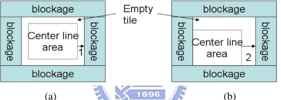
e straight implementation, without overlapping any gridline, and has the same distance to PMT boundary (Figure 10(a)). In original implementation, the center line area overlaps gridlines on bottom or left side, and distance to PMT boundary is different (Figure 10(b)).

After we modified the implementation, all center points’ coordinate of pins that always are even will generate gridlines that always are odd coordinate due to contours. And for using space more efficient, we will let the center lines always go through the boundary of center line area in a PMT (Figure 10(a)). Then all center lines’ coordinate of nets are even. Now the gridline system is clear that all coordinate of gridlines are always odd, and all center lines’ coordinate of nets are even.

Implementation Issues

3.1 Implementation of non-zero width wire model

The original implementation of non-zero width wire model in NEMO did not do straight as the way showed in Figure 9(a). Instead of shrinking the contour width by a half unit width, it only shrinks left and bottom boundary of the contour by a unit width (Figure 9(b)). When NEMO read input, it will multiple all input coordinate by 2, and then all coordinate of pins are even, a unit width is 2,and a half unit width is 1 in the routing system. Although these two kinds of implementations will lead to the same result, the original way makes people confused easily. In Figure 10, shows where a center line can pass in a PMT with adjacent blockages. In th

3.2 Enhancement of path search

(a) (b)

Figure 9 Two implementation (a) Contours will be shrunk by a half unit width (b) Only left and bottom boundaries shrink a unit width.

(b) (a)

Figure 10 Center line area in a PMT (a) straight implementation (b) original implementation

ing and construction

segments. Our cost function is defined as p+ np+ v, where p is length of

preferred segments, np is length of non-preferred segments, v is number of vias and α、β、γ are constants and α<γ<β. Before we add overlap area information, path

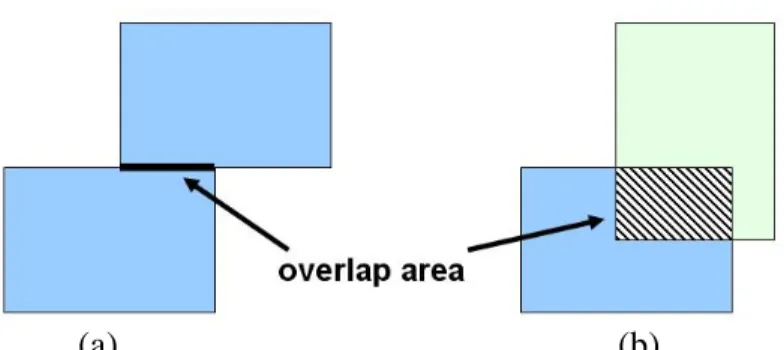
We add extra information in tiles to record the overlap area with other tiles when tiles propagate. If last tile is in the same layer, the overlap area is a line; if last tile is in different layer, the overlap area is a rectangle that showed as Figure 11. It can help us estimate path cost accurately and construct path correctly when there exist non-prefer

cost was over-considered when count non-prefer segments in tile propagation because original path cost only depends on the location of entry points, which mentioned at section 2.2. Figure 12 showed an example that how the cost is over-considered, when we propagate from tile1 to tile3, the minimum cost path only has a short non-prefer cost in tile1 (Figure 12(a)), but if we estimate cost only by entry point, there is a redundant non-prefer segment cost in tile2 (Figure 12(b)). After we record overlap area, we have complete information in estimating path cost. In Figure 12(c) when we propagate to tile3, we can find the two overlap areas are overlapped in x-coordina

then we will count the cost of the horizontal segment in tile

te,

and 2 as a preferred

segment. Because we know the region of overlap area and we can estimate that the

ect bac nt. When we connect path from tile2 to tile1, if we only consider entry points’ information, we will connect entry point3 to entry point2 and can not get

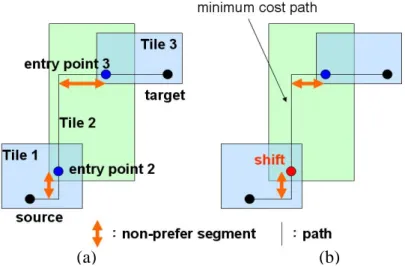
inimum cost path. When we have information of overlap area, we know entry e constructed as showed in (Figure 13(b)).

entry point of tile2 can shift right and the horizontal segment will on tile1 not tile2 when path construct.

In path construction, information of overlap area will lead us construct a minimum cost path. If we only have information of entry points, we will construct a path as showed in Figure 13(a). We construct path from target pin, and then conn

k to last entry poi

a m

(a) (b)

Figure 11 Overlap area (a) two tiles are in the same layer (b) two tiles are in different layer

(a) (b) (c)

Figure 12 Estimating cost in tile propagation (a) a possible minimum cost

estimate cost accurately

path only has a non-prefer segment cost in tile1 (b) only use entry points we will overconsider cost (c) with complete overlap information we can

3.3 Wire refinement

NEMO apply pin-to-pin routing, so some segments of a multi-pin net could cover each other or have design rule viol

(a) (b)

Figure 13 Path Construction (a) We can not find a minimum cost path only with information of tiles and entry points (b) If we know overlap information, entry poin2 will shift to right, and then we find a minimum cost path

n. We solve this problem case by case after

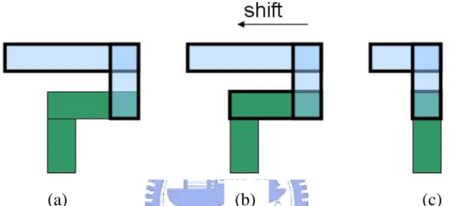
ntal segments at layer1 that produce space rule violations. We find a rule to solve this kind of cases. First we try to find a short vertical segment at layer1 which attached a horizontal segment at the same layer (Figure 15(a)) and then search other two-pin nets for a horizontal segment at the same layer that attach the vertical segment at the other head(Figure 15(b)). And then we will shift the vertical segment right or left to reduce this violation as Figure 15(c). This rule can apply on any layer, horizontal or vertical layer, Figure 16 shows that how it works in vertical layer.

atio routing process.

(a) (b) Figure 14 Two cases of space violation

(a) (b) (c)

Figure 15 Steps to Rule1 (a) Find a short vertical segment in horizontal layer which attach a horizontal segment. (b) Search other two-pin nets for a horizontal segment attaching at the other head of the vertical segment. (c) Shift the vertical segment left and then violation clear.

(a) (b) (c)

Figure 16 Rule1 apply to vertical layer (a) Find a short horizontal segment in vertical layer which attach a vertical segment. (b) Search other two-pin nets for a vertical segment attaching at the other head of the horizontal segment. (c) Shift the horizontal segment up and then violation clear.

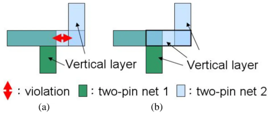
Another kind of common cases is like Figure 17(a). The horizontal segments of two two-pin nets overlap each other and the two attached vertical segments have space violation at the two corners. We solve this case by changing the endmost part of the longer horizontal segment to vertical layer as showed in Figure 17(b). This rule also can apply on different direction as Figure 18 showed.

One more kind of cases showed as Figure 19(a). A horizontal segment attached a short vertical segment has space violation with the other horizontal segment. After we change the short segment to horizontal layer

(a) (b)

Figure 17 (a) A case with space violation (b) Reduce the violation by changing the endmost part of the longer horizontal segment to vertical layer.

(a) (b) (c)

Figure 18 Rule2 apply on different direction (a) left (b) down (c) up

(a) (b)

Figure 19 (a) A case with space violation (b) After we change the short vertical segment to horizontal layer, there is no violation.

Chapter 4

Tool integration

4.1 Nets decomposition

topology, separating a net into two-pin nets before global routing stage will not benefit by this character. Below I will explain how we divide a steiner tree topology, a result of global router, and separate it into two-pin pairs.

The global router returns a steiner tree that comprises many dot-to-dot segments, a dot may be a steiner point or a pin. First we categorize all dot-to-dot segments into three types：pin to pin as type0, pin to steiner point as type1 and steiner point to steiner point as type2. All type0 segments already connect two pins so we only need to handle type1 and type2 segments. We start from a type2 segment (Figure 20(b)) and extend from one end until attached a type1 segment, e.g. find a pin (Figure 20(c)) and then we extend from the other end (Figure 20(d)), and then we get a pin-to-pin pair and path. We call this kind of two-pin nets a trunk. After we get a trunk we extend from its’ steiner point to get other two-pin nets called a branch. A branch record the path extending from a steiner point to a pin, and we will take a pin of the trunk that is nearest to the steiner point as the other pin of the pin pair of the branch (Figure 21). This is for the pseudo pin-to-path routing in NEMO, which mentioned at section 2.2. If there is no type2 segment, we can form a trunk from a type1 segment (Figure 22). And if a branch has any steiner point, we will get sub-branches from it.

(a) (b) (c) (d) Figure 20 Separate a steiner tree into two-pin nets (a) A steiner tree with

one end (d) extend from the other end and get a trunk.

many dot-to-dot segments (b) start from a type2 segment (c) extend from

(a) (b) (c)

Figure 21 Separate a steiner tree (continued) (a) find a branch from a steiner point of the trunk (b) find an other branch (c) branches record path extending from steiner point and a addition pin of trunk.

(a) (b) (c)

Figure 22 Separate a steiner tree (continued) (a) find an other trunk from a type1 segment (b) get a trunk (c) find a branch and stop the separating process.

4.2 Tool design flow

The design flow is showed as Figure 23. We maintain a routing database that initially record the input information, and then give global router necessary information to produce topology. After separate steiner tree topology into two-pin nets topology, NEMO will query data from routing databas and then start detailed routing.

Final ow

on th d a routing result. As the

figure you can see that there are some buttons at left-top, they are open file, routing e

ly the routing result that already fixed will save in the routing database and sh e screen. Figure 24 shows the screenshot of the GUI an

, fit, zoom-in, zoom-out, and redraw. And at right, you can see the control panel from top to down：cursor coordinate, metal and via layer checker buttons (choose to show) and routing result information.

Chapter 5

Experiment Results

To compare with old version NEMO, we perform this tool on a 1.2GHz Sun Blade-2000 workstation with 2GB memory. We route ISCAS89 benchmarks showed as Table 1; “#Lay” shows the number of available routing layer; “#2-pin nets” shows the number of two-pin connections after net decomposition. Table 2 shows the result of old version NEMO with an old version global router, and result of this work with a new global router. In this table, “# of Vias” shows the number of vias, “WL” shows the total wire length in micrometer, “Non-prefer” shows the non-prefer length in micrometer and the percentage of WL. Compare with old version, we can see that non-prefer length are reduced at all six cases and run time are reduced at large test cases. Due to precisely estimating path cost, non-prefer length should be reduced. And accurately constructing minimum cost paths is helpful to reduce the run time when

uting a large case.

Table 1. Statistics of ISCAS89 series benchmark circuits

Circiut Size(μm) Pins # Lay # 2-pin nets

ro s9234 4040×2250 4260 3 2774 s5378 4350×2390 4818 3 3124 s13207 6600×3650 10776 3 6995 s15850 7050×3890 12793 3 8321 s38417 11440×6190 32344 3 21035 s38584 12950×6720 42931 3 28177

Table 2. Comparison of the rout eries benchmarks

NEMO (old ve NEMO (this version)

ing result of ISCAS89 s rsion) Time(s) # o Via WL (μm) Non-prefer f s WL (μm) Non-prefer Time(s) # of Vias s9234 2.09 5885 5.5e4 591 1% 2.79 6310 5.8e4 103 0.2% s5378 2.95 6951 7.5e4 790 1% 3.93 7388 7.7e4 199 0.3% s13207 7.87 15098 1.8e5 1482 0.8% 9.95 15993 1.8e5 76 0.0% s15850 21.68 18019 2.2e5 1546 0.7% 10.93 18740 2.3e5 435 0.2% s38417 38.73 49117 4.8e5 16908 3.5% 31.23 47215 5.0e5 1350 0.3% s38584 70.03 59956 6.7e5 4942 0.7% 53.01 63502 6.9e5 1497 0.2%

Table 3. Statistics of Ibm-series Benchmark circuits

Circiut Size(μm) Pins # Lay # 2-pin nets Ibm01 7676*7678 44265 4 32758 Ibm02 8745*8753 78170 5 59741 Ibm07 12745*12751 164368 5 119974 Ibm08 13246*13255 198179 5 150235 Ibm09 13444*13446 187871 5 137478 Ibm10 17233*17231 268999 5 204772 Ibm11 15187*15193 237061 5 170045 Ibm12 18540*18541 294185 5 226446

Besides we route the ISPD98 benchmarks [15], which originally only provide partition information, but people set some detail information for placement. We use the result of a placer ragon [16 ich generate

route these benchma workstatio th AMD Opte n 2.0GHz processor and 16GB me . We modify some routing information for NEMO. First the pins are a line not a point, NEMO can not handle ituation yet, s ed t ns to a point. Second, all layers have different rule but for convenience and simplification we ade all layers with the same rule. Table 3 lists the statistics for eight circuits of

arks. Our result is showed as Table 4, and we compare it with the sult of a commercial tool called Nanoroute. Only the first case we have shorter run time, and it shows that our tool need much more time to handle dense cases. We may called D ], wh s LEF/DEF output files, and

rks on a n wi ro mory this s o we chang he pi m ISPD98 benchm re

improve that by a better rip-up and reroute method. Wire length is similar, but we

roduce 0% s m han e. W k i y be sed d

wire refinement. Our wire refinement just handles a few cases for DRC, and there still exist many redundant wires and vias in the final result. We

, esu ld les e th onl tle via an

result of Nanoroute.

. C ris the seri u res

Our Tool Commercial Tool

p about 1 via ore t Nanorout e thin t ma cau by the ba

believe if we can solve this problem the r lt shou have s wir leng and y a lit more s th the

Table 4 ompa on of Ibm es ro ting ult

Global Detailed # of WL Gl routing time m:ss) r Vias ) obal routing time (mm:ss) Detailed ting time (mm:ss) # of WL μm) (m outing time (mm:ss) (μm rou Vias ( ibm01 00:01 01:07 117221 7.3e5 00:05 02:26 102106 7.8e5 Ibm02 00:02 17:49 267496 2.0e6 00:37 03:56 238484 2.2e6 Ibm07 00:05 48:54 531796 4.4e6 00:59 10:29 468562 4.4e6 Ibm08 00:07 40:03 626731 4.8e6 00:44 06:57 563441 4.8e6 Ibm09 00:04 16:08 531335 3.9e6 00:28 05:30 478666 3.8e6 Ibm10 00:10 73:22 829871 7.3e6 00:56 09:14 745601 7.2e6 Ibm11 00:08 30:57 684663 5.6e6 00:44 08:37 618555 5.5e6 ibm12 00:21 X X X 01:42 16:44 903122 1.0e7

Chapter 6

Conclusions

We improve and enhance NEMO’s structure in the aspect of gridline system, path searching and construction. The gridline system is clear in present

plementation. And path searching is estimated pre uction is

tel to rec addi iles orma utpu atio E

will be m by n rule checker and s generate a DRC free result.

we bine ges iv lobal ter wi EMO a

position process. Finally ck rogra s a routing tool w raphic nter hich p es ba pl erati ch as z

im cisely and constr

accura y due odified

ording a desig

tion t inf tion. O olver to

t inform n of N MO

Also com a con tion-dr en g rou th N by net

decom we pa all p ms a ith a g

Chapter 7

Bibliography

[1] J. Cong,

[4] R. E. Lunow, “A Channelless, Multilayer Router,” in 25th ACM/IEEE Design Automation Conference, pp. 667-671, 1998.

[5] C.-C. Tsai, S. Chen, and W. Feng, “An H-V Alternation Router,” IEEE

Transactions on Computer-Aided Design of Integrated Circuits and Systems Vol.

11(8), pp. 976-991, August, 1992.

[6] J. Dion and L. M. Monier, “Contour: A Tile-based Gridless Router,” Western Research Laboratory Research Report 95/3, Palo Alto, California.

] L.-C. Liu, H.-P. Tseng, and C. Sechen,”Chip-level area routing,” in Proc. Int.

Symp. Physical Design, Apr. 1998, pp. 197-204.

[8] Z. Xing and R. Kaog, “Shortest Path Search Using Tiles and Piecewise Linear Cost Propagation,” IEEE Transactions on Computer-Aided Design of Integrated

Circuits and Systems, Vol. 21, No.2, pp. 145-158, Feb. 2002.

J. Fang, and K. Khoo, “DUNE: A Multi-Layer Gridless Routing System with Wire Planning,” IEEE Transactions on Computer-Aided Design of Integrated

Circuits and Systems, Vol. 20, No. 5 pp. 633-646, May, 2001.

[2] M. Sato, J. Sakanaka, and T. Ohtsuki, “A fast line-search method based on a tile plane,” in IEEE Int. Symp. Circuits and Systems, May 1987, pp. 588-591.

[3] A. Margarino, A. Romano, A. De Gloria, F. Curatelli, and P. Antognetti, “A tile-expansion router,” IEEE Transactions on Computer-Aided Design of Integrated

Circuits and Systems, Vol. CAD-6, pp. 507-517, July 1987.

[9] T. Ohtsuki, “Gridless ro uting algorithms based on

computational geometry,” in Pr , May 1985, pp.

802-809

0] S. Q. Zheng, J. S. Lim, and S. Iyengar, “Finding obstacle-avoiding shortest paths

near shortest paths and

ded Design of Integrated Circuits and

Multi-Layer Planes and Pseudo-Tile Propagation,” uters ─ New wire ro

oc. Int. Conf. Circuits and System

[1

using implicit connection graphs,” IEEE Transactions on Computer-Aided Design of

Integrated Circuits and Systems, Vol. 15, pp. 103-110, Jan. 1996.

[11] Y. Wu, P. Widmayer, M. Schlag, and C. Wong, “Rectili

minimum spanning trees in the presence of rectilinear obstacles,” IEEE Trans.

Comput., Vol. C-36, pp. 321-331, Mar. 1987.

[12] J. Cong, J. Fang, and K. Khoo, “An implicit connection graph maze routing algorithm for ECO routing,” in Proc. Int. Conf. Computer-Aided Design, Nov. 1999, pp. 163-167.

[13] J. Ousterhout, “Corner stitching: A data-structuring technique for VLSI layout tools,” IEEE Transactions on Computer-Ai

Systems, Vol. CAD-3, pp.87-100, Jan. 1984.

[14] Y.-L. Li, H.-Y. Chen, and C.-T. Lin, “NEMO: A New Implicit Connection Graph-Based Gridless Router with

IEEE Transactions on Computer-Aided Design of Integrated Circuits and Systems,

Vol. 26, No.4, pp. 705-718, Apr. 2007.

[15] http://vlsicad.ucsd.edu/UCLAWeb/cheese/ispd98.html [16] http://er.cs.ucla.edu/Dragon/