應用ESIF陣列技術來改善語音的品質

國

立 交 通 大 學

機械工程學系

碩士論文

應用

ESIF 陣列技術來改善語音的品質

Speech Enhancement using Equivalent Source Inverse Filtering

-Based Microphone Array

研

究 生: 何克男

指導教授

: 白明憲

Speech Enhancement using Equivalent Source Inverse Filtering

-Based Microphone Array

研 究 生：何克男 Student：Kur-Nan Hur

指導教授：白明憲 Advisor：Mingsian R. Bai

國 立 交 通 大 學

機械工程學系

碩 士 論 文

A thesis

Submitted to Department of Mechanical Engineering

Collage of Engineering

National Chiao Tung University

In Partial Fulfillment of Requirements

for the Degree of Master of Science

in

Mechanical Engineering

July 2009

HsinChu, Taiwan, Republic of China

中華民國九十八年七月

應用

ESIF 陣列技術來改善語音的品質

研究生：何克男

指導教授：白明憲 教授

國立交通大學 機械工程學系 碩士班

摘 要

本論文提出一種新的麥克風陣列技術運用聲學信號處理方法而

實現在電信通訊系統中，此技術稱為聲源等值反濾波器設計演算法。

單進多出聲源等值反濾波器設計演算法(SIMO-ESIF)的目的在於在充

滿迴響的環境裡能夠重建語音訊號，此系統能夠達到兩個重要的目

標：抑止殘響和消除噪音。其適用的電信通訊系統如車內免持聽筒的

系統，在密閉的車子環境裡所收到的語音通常夾雜著許多背景噪音且

需要被改善，此演算法結合提出的

GSC 演算法是為了進一步在更嚴

重迴響的環境裡改善噪音消除的效果。主觀測試的結果用變異數分析

方法來做為分析的工具。進一步使用

Fisher’s LSD

分析法來證明新提

出的方法在改善含有噪音的語音訊號上效果有明顯的進步並且提供

更棒的音質。

Speech Enhancement using Equivalent Source Inverse Filtering

(ESIF) Array

Student: Kur-Nan Hur Advisor: Mingsian R. Bai

Department of Mechanical Engineering National Chiao-Tung University

A

BSTRACT

New microphone array techniques are proposed in this paper for acoustic signal processing in telecommunication application. These endeavors are based on the central idea of Equivalent Source Inverse Filtering (ESIF). The single input multiple output equivalence source imaging (SIMO-ESI) algorithms are suggested to reconstruct the speech signal in a reverberant environment. Specifically, the system serves two purposed: dereverberation and noise reduction. It has promise in telecommunication application such as the automotive hands-free system, where noise-corrupted speech signal often needs to be enhanced. In order to further improve the noise reduction performance in spatial filtering and robustness against system uncertainties, the SIMO-ESIF algorithm is combined with an adaptive Generalized Side-lobe Canceller (GSC). The system is implemented on an NI-PXI platform and evaluated experimentally in car environment. As indicated by several performance measures in noise reduction and speech distortion, the proposed microphone array algorithm proved effective in reducing noise in human speech without significantly compromising the speech quality. The results of subjective tests were processed by using analysis of variance (ANOVA) to justify the statistic significance. A post-hoc test Fisher’s LSD was conducted to further assess the pairwise difference between the NR algorithms.

誌謝

短短兩年的研究生生涯轉眼即逝。在此感謝白明憲教授的諄諄教誨與照顧， 在白明憲教授的指導期間，深刻的感受到教授對於追求學問的熱忱，更是佩服教 授淵博的學問與解決問題的方法。在教授豐富的專業知識以及嚴謹的治學態度 下，使我能夠順利完成學業與論文，在此致上最誠摯的謝意。 在論文寫作方面，感謝本系鄭泗東教授和陳宗麟教授在百忙中撥冗閱讀，並 提出寶貴的意見與指導，使得本文的內容更趨完善與充實，在此學生致上無限的 感激。 在這兩年的研究生生涯中，承蒙博士班陳榮亮學長、林家鴻學長，以及已畢 業的李志中學長、施畊宇學長、洪志仁學長、謝秉儒學長、劉青育學長、黃兆民 學長在研究與學業上的適時指點，並有幸與王俊仁同學、郭育志同學、艾學安同 學、劉冠良同學互相切磋討論，讓我獲益甚多。此外學弟妹陳俊宏、廖國志、廖 士涵、曾智文、桂振益、張濬閣、劉孆婷以及學姐李雨容在生活上的朝夕相處與 砥礪磨練，亦值得細細回憶。因為有了你們，讓實驗室裡總是充滿歡笑與淚水。 能順利取得碩士學位，要感謝的人很多，上述名單恐有疏漏，在此一併致上我最 深的謝意。 最後僅以此篇論文，獻給我摯愛的家人。感謝奶奶何張沙、外婆李賴秀瓶女 士，您們慈祥的笑容及呵護，總是讓我有勇氣繼續前進。感謝母親李淑惠女士、 父親何炳純先生，哥哥何克凡，你們對我無微不至的包容與諄諄教誨，讓我不至 於迷失了方向。感謝女友林寶珠總是陪伴在我身邊，聽我大吐苦水並給我最真摯 的加油鼓勵。這一路上，因為有你們的付出與支持，給了我最大的精神支柱，也 讓我有勇氣面對更艱難的挑戰。

T

ABLE OF

C

ONTENTS

摘 要 ...i

ABSTRACT...ii

誌謝... iii

TABLE OF CONTENTS...iv

LIST OF TABLES...v

LIST OF FIGURES...vi

I. INTRODUCTION...1

II. EQUIVALENT SOURCE INVERSE FILTERING...3

III. SIMO-ESIF WITH GSC ...4

1. Griffiths-Jim beamformer (GJBF) structure ...5 

2. LAF-LAF structure ...6 

3. Robust GSC using linear algebra...7 

3.1 The design method of blocking matrix ...7

3.2 Signal processing in Multiple-Input Canceller ...9

IV. ARRAY PERFORMANCE MEASURES...9

V. OBJECTIVE AND SUBJECTIVE EVALUATIONS ...10

1. Objective evaluation ...11 

2. Subjective evaluation...13 

VI. CONCLUSIONS ...14

ACKNOWLEDGMENTS ...15

L

IST OF

T

ABLES

TABLE I The descriptions of six proposed algorithms. ...18 TABLE II The performance of the six proposed algorithms in terms of the objective measures...19 TABLE III. The MANOVA output of the listening test of the six proposed algorithms. Cases with significance value p below 0.05 indicate that statistically significant difference exists among all methods...20

L

IST OF

F

IGURES

FIG. 1 The block diagram of SIMO-ESIF algorithm.

FIG. 2 The block diagram of the generalized sidelobe canceller. FIG. 3 The block diagram of GJBF structure.

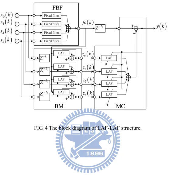
FIG. 4 The block diagram of LAF-LAF structure.

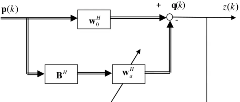
FIG. 5 The block diagram of SIMO-ESIF-GSC algorithm.

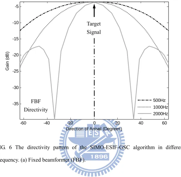
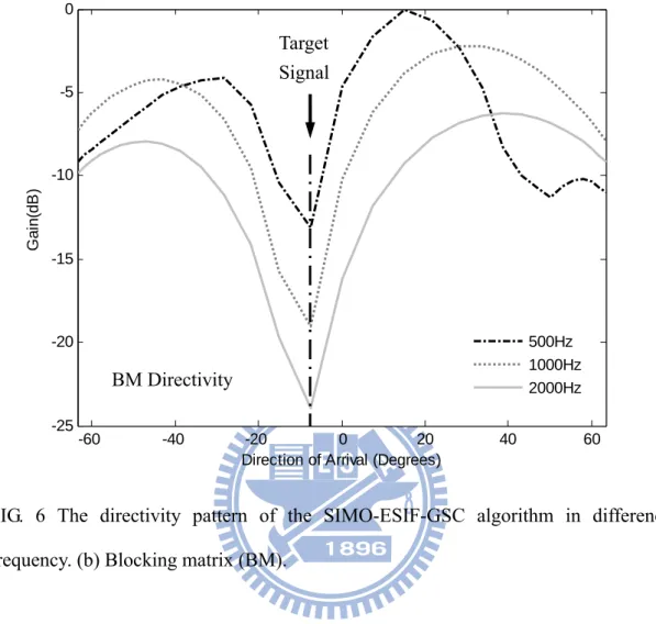
FIG. 6 The directivity pattern of the SIMO-ESIF-GSC algorithm in difference frequency. (a) Fixed beamformer (FBF). (b) Blocking matrix (BM).

FIG. 7 The compared beam pattern of the GJBF, LAF-LAF and SIMO-ESIF-GSC algorithm in 500 Hz.

FIG. 8 The experimental arrangement inside the car.

FIG. 9 The performance of SIMO-ESIF algorithm and SIMO-ESIF-GSC algorithm in three different designed methods. (a) PIF algorithm compared with GSC-PIF algorithm. (b) MIF algorithm compared with GSC-MIF algorithm. (c) MTR algorithm compared with GSC-MTR algorithm.

FIG. 10 The comparison of the six proposed algorithms. The results of the listening test are processed by using the MANOVA.

I. INTRODUCTION

In recent year, microphone arrays have been widely studied for teleconferencing, telecommunication, speech recognition, speech enhancement, and hearing aids. In these applications, effective communication in noisy environments has been one of the pressing problems. The delay-and-sum-beamformer has been widely researched for speech recognition and noise reduction, which verified that it only performed well for uncorrelated noise [1]. The standard superdirective beamformer is another classic technique to investigate these problems. The result shows that it gets better performance only for diffuse noise [1]. However, both of them have been applied to noise reduction rather than to dereverberation.

In some environments such as in a car cabin, the speech signals are corrupted not only by background noise but also serious reverberation. Adaptive microphone arrays are especially promising system in terms of interference reduction [1]-[9]. The potential for using adaptive beamforming to improve the performance of sensor arrays was recognized in the early 1960’s in the fields of sonar [10]-[13], radar [14]-[16], and seismic [17]-[19] signal processing. It soon became apparent that a variety of formulations of optimum detection and estimation problems gave rise to the same spatial processor. The basic concept is to use measured background spatial correlation characteristics to reject noise and interference, thereby improving beam output signal-to-noise ratio. Generalized sidelobe canceller (GSC) is an adaptive beamforming that can attain high interference-reduction performance with a small number of microphones arranged in small space. It is very sensitive to the room reverberation, steering and calibration error. Any of these disturbances cause

cancellation and distortion of the desired signal. Adaptive beamformers extract the signal from the direction of arrival (DOA) specified by the steering vector, which is a parameter of beamforming. Many robust adaptive beamforming techniques have been proposed to avoid signal cancellation. Griffiths-Jim beamformer (GJBF) [2] is an adaptive beamformer based on the GSC which target-signal cancellation occurs in the presence of steering-vector errors. The steering-vector errors are caused by errors in microphone positions, microphone gains, reverberation, and target direction. But it can be shown that this kind of algorithms fails in reverberant environments [3].

In this paper, a new microphone array techniques is proposed for acoustic signal processing in telecommunication application. An ESIF technique is proposed to identify locations and strengths of speech sources [4]. However, a serious reverberant phenomenon is always produced by the acoustical environment. The inverse filters based on the measured plant can eliminate the reverberation effectively. They can also suppress interfering signals and enhance the acquired target speech signals. In addition, a new robust adaptive beamformer based on multiple linear equality constraints is proposed to enhance the interference of side-lobe further. They were introduced by Frost [8] in his recursive adaptive beamforming algorithm. A useful implementation of the linearly constrained minimum variance (LCMV) is the GSC which relies on optimizing the filter in two mutually orthogonal subspaces [9]. The proposed blocking matrix (BM) of GSC is designed according to these subspaces, which places beam pattern nulls in interference directions and controls mainlobe. A leaky coefficient adaptation algorithm called leaky LMSis used for the adaptive filter in the multiple-input canceller (MC) [20]-[21]. A large leakage is needed to allow a large look-direction error, leading to degraded interference reduction.

The proposed approaches have been implemented in a real car by using the multi-channel data acquisition system. The objective and subjective tests were

carried out to evaluate the proposed algorithms. Objective measures are utilized for evaluating the performance of the proposed algorithm [22]. In addition, listening tests were conducted to assess the subjective performance of the proposed system. In order to justify the statistical significance of the results, the data of subjective listening tests are processed by the multivariate analysis of variance (MANOVA) [25] method, followed by the least significant difference method (Fisher’s LSD) as a post

hoc test.

II. EQUIVALENT SOURCE INVERSE FILTERING

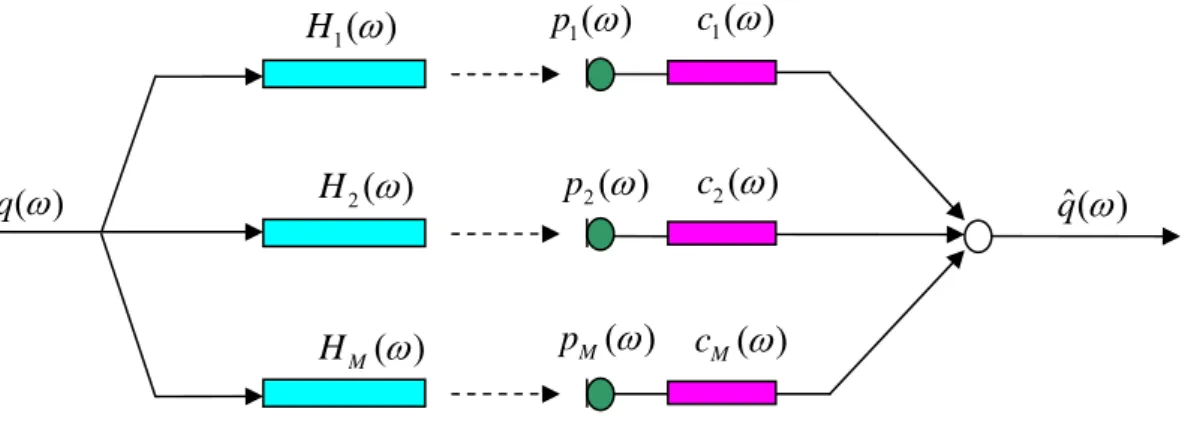
The formulation of SIMO-ESIF technique is presented in this section. The block diagram of the SIMO_ESIF with M microphones is shown in Fig. 1. Assume there is a fixed source in the system.

The measured sound pressures and the source strengths are related in matrix form

p = Hq , (1) where ( )pn ω is the signal received at the nth microphone and Hn( )ω is the plant

between source and the nth microphone. q( )ω is the Fourier transform of a scalar source fixed in the space. In the frequency domain, Eq. (1) can be written as follows

( ) qω = p H , (2) where,

[

1( ) ( )

]

T M p ω p = p ω (3)

[

1( ) ( )

]

T M H ω H ω = H (4)

[

1( ) ( )

]

T M c ω c ω = c (5) The aim here is to estimate q( )ω based on the measurement p. This can be regarded as a model matching problem. An inverse filter such that can be found as follows

ˆq= cp cH= q≈q (6)

In order to estimate the source signal q( )ω , it can be considered as an optimization problem 2 2 min q p - Hq (7)

The Eq. (7) shows an underdetermined problem which has infinite solution. The minimum norm solution to the problem above is given as

1 2 ˆ ( ) H H 2 H T q= H H H p− =H p =c p , (9)

where the optimal inverse filter is H H 2 2 T = H c (10) H

If H 2₂ is omitted, the inverse filter above reduces to the “phase-conjugated” filter,

or the “time-reversed” filter. However, for the point source model in SIMO array, it straightforward is to show that 2 2 1 m= rm

∑

H , (11) where r_m is the distance between source and the mth microphone. Since

2 1 M = 2 2 H is a

frequency-independent constant, the inverse filters and the time-reversal filters differ nly a constant scaling in the point source model.

III. SI o

MO-ESIF WITH GSC

The design of the SIMO-ESIF with Generalized Side-lobe Canceller (GSC) is introduced in this section. The speech signals are degraded by background noise in the automotive hands-free system, which causes communicational quality to be

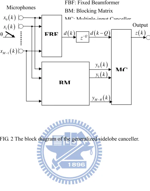
hampered. The GSC technique is proposed as a further processing after SIMO-ESIF algorithm, which increases directivity of main-lobe by suppressing the interference of side-lobe. A structure of the GSC with M microphones is shown in Fig. 2. It comprises a fixed beamformer (FBF), a multiple-input canceller (MC), and a blocking matrix (BM). The FBF is designed to form a beam in the look ion so that the target signal is passed and all other signals are attenuated. The _m( )

direct

x k is the output

gnal of the mth microphones and d k( ) is the output of the FBF at the time sample k . The MC is composed of multiple adaptive filters which generate replicas of

components correlated with the interferences. It adaptively subtracts the components correlated to the output signals _m( )

si

y k of the BM from the delayed

output signal d k( −Q)of FBF, where Q is the number of delay samples for

causality. Contrary to the FBF, the BM forms a null in the look direction so that the target signal is suppressed and all other signals are passed though. It rejects the interferences which is obtained from the output signals of BM and extracts the target signal. In conclusion, in the subtractor output z k( ), the target signal is enhanced

nd undesirable signals such as ambient noise and interferences are suppressed.

1.Griffiths-Jim beamformer (GJBF) structure

acent microphones can be used a

(12) whe

a

Figure 3 shows the structure of the GJBF. The FBF is the aforementioned inverse filter. The BM is a delay-and-subtract beamformer as shown in Figure3. Assuming a look direction perpendicular to the array surface, no delay element is necessary. Thus, a set of subtracters which take the difference between the signals at the adj

s a BM. The outputs of BM are described as follows:

1 ( ) ( )

n n

z ( )k =x k −x_n+ k

The adaptive filters of the MC are using least- mean-square (LMS) algorithm, which can be obtained as follows:

(

1

)

1

( ) ( )

0 ( ) N T n n n y k fo k L k k − = = − −

∑

w z (13)

(

1

)

( )

( ) ( )

n k+ = n k +μy k w w z_n k (14)

( )

( )

( )

( )

( )

2 ,0 , ,1 , , , 1 T n n n n M T k w k w k w k k − ⎡ ⎤ ⎣ ⎦ w

( ) (

, 1 , ,

)

(

2 1

)

n ⎡⎣zn k zn k− zn k−M + ⎤⎦ z where

[ ]

T

i denotes vector transpose and MC btrsu act form fo k

(

−L₁

)

the

components correlated with z_n

( ) (

k n=0, ,N− . 1

)

M is the number of taps in ₂

each adaptive filter, and w_n

( )

k and z_n

( )

k is the coefficient vector and the signal

ector of the n th adaptive filter, respectively. y k

( )

v is the output subtracter

2. LAF-LAF structure

e 4 shows its block diagram. The th output of the BM can be obtained as follows:

.

A target-tracking method with leaky adaptive filters (LAF) in the BM is proposed as a solution to target signal cancellation. It combined with leaky adaptive filters in the MC, thereby called a LAF-LAF structure. Figur

n

(

)

(

)

( ) ( )

( )

( )

( )

1

( )

2 ,0 ,1 , 1 1 1 , , , 1 T n n n T n n n n M T z k x k L k k k h k h k h k M − + = − − ⎡ ⎤ ⎣ ⎦ + h fo h

( )

k _⎣⎡fo k

( ) (

, fo k−1 , ,

)

fo k

(

−

)

⎤_⎦ fo similar to th ilters in GJBF, (15)

e adaptive f h_n

( )

k is the coefficient vector of the n th

LAF, and fo

( )

k is the signal vector consisting of delayed signals of fo k

( )

. Each

The adaptation by the LMS algorithm is described as follows:

)

(

1

( )

( ) ( )

n + = n k +αz k n k

h k h fo (16)

where α is the step size for he adaptation algorithm.

The LAFs in the BM alleviate the influence of phase error, which results in the robustness. The LAFs also used in the MC for enhancing the robustness obtained in the BM. Thus, the LAF-LAF structure adaptively controls the look direction. Due to robustness by the adaptive control of the look direction, the LAF-LAF structure does not lose degrees of freedom for interference reduction. This structure can pick up a

rget signal with little distortion.

3. Robust GSC using linear algebra

3.1 The design method of blocking matrix

inimizing the output power subject to ultiple linear equality constrain

ta

The target of robust GSC is to minimize the array output power such that unity gain at the look direction is obtained. The design of the proposed robust beamformer can be formulated as one of m

m ts as follow

{ }

2 min | | H xx = E z w R w min w w (17) ubject to tri S 1 H g (18) where { H } E =

R x x is the data correlation ma x, =

w

g

is the impulse response of the

signal path from source to each microphone, w is the digital filter of the proposed GSC system, zis the output signal. The block diagram is shown in Fig. 5. Standard

which is a fixed filter and dependent on the data correlation matrix R. The optimal filter w may be decomposed into two mutually orthogonal subspaces: the constraint

ace R(g) and th

GSC implementation, a blocking matrix B is eeded to pro

sp e orthogonal space N(gH), i.e.,

w (19) Where w0 ⊥v . As a key in proposed

0− = w v

n duce the vector v, so that = v Bw (20) Such that ( ) a H N ∈

v g is satisfied and the constraint is not affected. is the daptive filter. The desired goal is

(21) e, the co a w a 0 0 ( ) 1 H H H H a a = − = − ≈ g w g w Bw g w g Bw

In principl lumns of B can be constructed from the basis vectors of ( H)

N g

such that _{g B 0 . To this end, each co mn of} H = _{lu Bmust be the null space of g ,} H

i.e., ( ) ( H)

R B ∈N g . The blocking matrix B can be o tained as follows: b

3 2 1 1 1 1 0 0 0 1 0 0 0 1 ⎢ ⎥ ⎣ _{⎦ (22)} The design goal of the BM is to form a null in the target direction so that target signal suppression can be achieved. The effect is demonstrated in Fig. 4, where directivity patterns of the FBF and the BM are illustrated. With the comparison of Figs. 6(a) and 4(b), the null of the BM and the mainlobe of the FBF are located in the target direction. The target signal has been successfully “blocked” at the main-lobe of the fixed array in different frequencies. In addition, there is an interested issue that with the comparison of other robust GSC technique, whether the proposed GSC

n a a a a a a ⎡_{− − −} ⎤ ⎢ ⎥ ⎢ ⎥ ⎢ ⎥ = ⎢ ⎥ ⎢ ⎥ ⎢ ⎥ ⎢ ⎥ B

technique can achieve the best performance or not. Two classic GSC technique called GJBF [2] and LAF-LAF [21] technique are selected to compare with the proposed GSC algorithm. Figure. 7 shows the beam pattern of the above algorithm in 500 Hz. The proposed GSC algorithm achieves the narrowest beamwidth in target

irection, which shows the highest interference reduction performance.

3.2 Signal processing in Multiple-Input Canceller

=0

delay samples f d

In the MC, leaky adaptive filters (LAF) [21] is used for enhancing the robustness obtained in the BM. LAFs subtract the components correlated to y_n

( )

k , (m ,…,N)

from d k

(

−Q

)

. Q is the number of or causality. Let M2 be the

number of taps in each LAF , and w_n

( )

k and y_n

( )

k are the coefficient vector and

the signal vector of the nth LAF, respectively. The signal processing in the MC can e obtained as follows:

(23)

⎦

(25)

The adaptation with the normalized LMS (NLMS) algorithm is described as: b

(

)

1

( ) ( )

0 ( ) N T n n n z k d k Q k k − = = − −

∑

w y (24)

( )

,0

( )

, ,1

( )

, , , 2 1

( )

T n k ⎡⎣wn k wn k wn M − k ⎤ w

( )

( ) (

, 1 , ,

)

(

2 1

)

n k ⎣⎡yn k yn k− yn k−M + ⎤⎦ y T

(

)

( )

( )

( )

( )

( )

1 n n T n j k j k y y z k k+ = k +μ k w w y (26) here

W μ is the step size for the adaptation algorithm.

IV. ARRAY PERFORMANCE MEASURES

performance[22]. The best way to quantify the amount of noise from an observed signal is the signal to noise ratio (SNR). With the first microphone as the reference,

e input SNR is defined as th 2 1 1 2 1 (dB) 10log { } SNR E v = , (23)

where x1 is the speech at microphone 1 and v1 is the noise at microphone 1. In order to know if the designed filte

{ }

E x

rs improve the SNR, the output SNR is defined after filter processing as follows:

c 2 A 2 { } (dB) 10 log { T } E c * v T E SNR = c * x (24)

R gain can be obtained by

The SN subtracting the output SNR from the input SNR.

A 1 (dB)

SNRG =SNR −SNR

e value of

ex to quantify the speech distortion called speech-distortion index (SDI) is defined (25) The higher th SNRG(dB), the more the noise is reduced. However, the maximizing (dB)SNRG is certainly not the best choice since the distortion of the

speech signal will likely be maximized as well. Therefore, an extremely useful ind as 2 1 2 1 { } (dB) 10log { } E x

The higher the value of SDI(dB), the less the speech signal is distorted. The relation between noise reduction and speech distortion is a trad m. By designing the FBF and controlli

T E x

SDI =

− c * x (26)

eoff proble

e adaptation of the MC, the can be proved with less distortion.

V.

ng th SNRG(dB)

im

OBJECTIVE AND SUBJECTIVE EVALUATIONS

environment, which is used to run the National Instruments Labview 8.6 data acquisition software. The measurement platform is NI-PXI 8105 controller13. The sound pressure data were picked up by using a linear 4-element microphone array. Figure. 8 shows the experimental arrangement inside the car. The PCB 130D20 microphones are used in the array. Microphones are equally spaced with 0.08m from each other. The target source is a male speech clip in English and the noise source is the white noise. The target source is located in front of the array at a distance of 0.4m. The noise source is placed 0.3m away from speech source. The sampling rate of speech signals is 8 kHz. Further, the proposed SIMO-ESIF algorithm is used as a beamformer in the FBF. The param ers in the Met C are: the length of wiener filter is 512 for the LAF’s and the step size μ is 0.001.

Objective and subjective experiments were undertaken to evaluate the presented methods, with results summarized in Table I. There are two different models employed to design the inverse filter: the ideal point source model and the measured plant in car environment. According to aforementioned section, the methods to design the inverse filter are: the inverse filtering technique and the time reversed filtering technique. The SIMO-ESIF and SIMO-ESIF-GSC methods are compared. The output signals in each proposed algorithm are evaluated objectively to compare the (dB)SNRG in interference reduction performance and SDI(dB) in speech

quality. The subjective listening test is employed to test which case can attain the est balance between noise reduction and speech distortion.

1. b

Objective evaluation

The preceding objective measures SNR1, SNRA, SNRG and SDI are employed to

assess the performance of six proposed algorithms, which are point-source-model-based inverse filtering (PIF), measured-plant-based inverse

filtering (MIF), measured-plant-based time reversed filtering (MTR), GSC combined with PIF (GSC-PIF), GSC combined with MIF (GSC-MIF) and GSC combined with MTR (GSC- MTR). The results of performance evaluation are summarized in Table II. First, in the comparison between SIMO-ESIF and SIMO-ESIF-GSC algorithms, it can obviously be observed from the SNRG that SIMO-ESIF-GSC algorithm is significantly better than the SIMO-ESIF algorithm in the aforementioned three designed methods with less speech distortion (SDI). Next, the point source model is compared with the inverse filter and the time reversal filter. The best performance in noise reduction is GSC-MIF method that attains 15.4 dB in SNRG. The inverse filtering approach has attained the highest SNR gain in a reverberant environment. With regard to speech distortion, the PIF method tends to get the least distortion, but the worst noise cancellation. According to all these grades, an expectable result can be obtained that noise reduction and speech distortion is a tradeoff. Figure. 9 compares the performance of SIMO-ESIF algorithm with SIMO-ESIF-GSC algorithm in three different designed methods, respectively. It can evidently show that the SIMO-ESIF-GSC algorithm perform better interference reduction in all the methods. The MIF and GSC-MIF methods seem to attain better noise cancellation with acc

ducing noise and interference without markedly compromising speech lity.

eptable speech distortion.

Overall, an obvious result can be revealed that both de-reverberation and noise reduction can be achieved by using the SIMO-ESIF technique. With the use of GSC, the performance of SIMO-ESIF can be further enhanced. According to the proposed BM approaches, the robust GSC exhibits the best performance in directional response and noise reduction. All this leads to the conclusion that SIMO-ESIF-GSC proves effective in re

qua

2.

lly significant. As for the

VL

Subjective evaluation

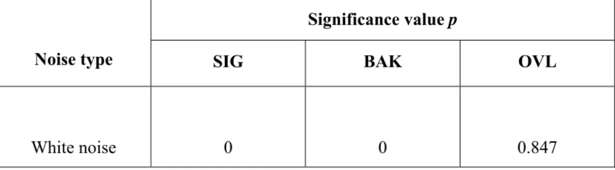
In order to further compare the preceding NR algorithms, subjective listening tests were conducted according to the ITU-R BS1116[24]. Fourteen participants in the listening tests were instructed with definitions of the subjective attributes and the procedures before the test began. The participants were asked to respond in a questionnaire after listening, with the aid of a set of subjective attributes measured on an integer scale from 1 to 5. The same six proposed algorithms used in the objective test are compared in this subjective test. The test signals and conditions remain the same as in the preceding listening tests. The reference is the signal received from microphone without any algorithm processing. The hidden anchor is the reference processed by using a lowpass filter. The mean and spread of the listening test results are shown in Fig. 10. In order to access statistical significance of the test results, the test results were processed using MANOVA15 with significance levels summarized in Table III. Cases with significance levels below 0.05 indicate that statistically significant difference exists among methods. Three subjective attributes employed in the tests, including signal distortion (SIG), background intrusiveness (BAK) and overall quality (OVL). From Table III, the difference of the indices SIG and BAK among the six proposed methods was found to be statistica

O , this observation is deemed statistically insignificant.

Next, a post-hoc Fisher’s LSD test was employed to perform multiple paired comparisons of the proposed algorithms. Post-hoc tests are generally performed after Analysis of Variance (ANOVA) which is able to determine whether or not significant difference is present in the data of a number of cases. The Fisher’s LSD test is one of the commonly used post hoc tests for the assessment of differences in the means between pairs of populations following the ANOVA test. In Fig. 10, surprisingly, in contrast to the results of objective evaluation, the GSC-MIF algorithm

performed quite poorly in SIG. The price paid for high noise reduction using the GSC-MIF algorithm is obviously the signal distortion, which was noticed by many subjects. For the SIG, the results of the post hoc test indicate that the grade of the GSC-PIF method is significantly higher than the grades obtained using the other methods. As for the BAK, the GSC-MIF method receives the highest grade among the other methods. Despite the excellent performance in SIG, the PIF algorithm received lower scores in BAK, which is consistent with the observation in the objective evaluation. In contrast with the PIF algorithm, the GSC-PIF algorithm improves SIG grade, which implicates the proposed GSC algorithm can enhance the performance of SIMO-ESIF algorithm. However, the grade in both SIG and BAK show no significant difference between MTR and GSC-MTR algorithms. It can be improved by selecting the different length of Wiener filter and the step size in MC. In addition, multiple regression analysis was applied to analyze the influence of SIG and BAK on OVL. The result exhibits that the effect upon SIG is bigger than BAK, but the difference between each other is not quite significantly. Therefore, there is no significant difference in OVL among all proposed algorithms, which indicated that the preference of each subjects is quite different. In general, the results of all the analysis lead to a common conclusion: the purpose of dereverberation and noise

duction can be achieved effectively in all the proposed methods.

VI.

IF combined with GSC achieves improved the perfo

re

CONCLUSIONS

A new microphone array technique called SIMO_ESIF algorithm is presented in this paper for noisy automotive environments. It is combined with the proposed GSC technique to eliminate the interference and improve speech quality. Experiment results show that SIMO_ES

The proposed algorithms have been compared with each other via extensive objective and subjective tests. These methods exhibit different degrees in trading off reduction performance and speech quality. The MIF and GSC-MIF algorithms seem to have achieve a good compromise between speech quality and noise elimination. It has been observed in an objective evaluation that SIMO-ESIF with proposed GSC

very effective in noise reduction with little speech distortion.

ACKNOWLEDGMENTS

Taiwan, Republic of hina, under the project number NSC 97-2221-E-009-010-MY3.

REFERENCES

[1] J.

eech recognition –a comparative study-,” in Proc.

[2]L

[3]

. EURASIP European

[4]M is

The work was supported by the National Science Council of C

Bitzer, K. U. Simmer and K. D. Kammeyer, “Multi-microphone noise reduction techniques for hands-free sp

ROBUST, 171–174 (1999).

. J. Griffiths and C. W. Jim, “An alternative approach to linear constrained adaptive beamforming,” IEEE Trans. Antennas Propagat., AP-30, 27-34 (1982). J. Bitzer, K. U. Simmer and K. D. Kammeyer, “Multichannel noise

reduction –algorithms and theoretical limits-,” in Proc Signal Proc. Conference (EUSIPCO), 1, 105-108 (1998).

nearfield equivalence source imaging: fundamental theory and implementation,”

[6]O

constrained adaptive filters,”

[7]Y icrophone array for car environment,” Speech Commun.,12, no. 1,

[8]O constrained adaptive array processing,”

[9]H ust adaptive beamforming,” IEEE

[10] n

[11] ptimum processing for acoustic arrays,” J. Brit. IRE, 26, no. 4,

[12]

for normal

[13] oise in a

[14] requency side-lobe canceller,” General Electric

[15] arrays by the Schwartz

[16]

J. Sound Vib. 307, 202–225 (2007).

[5] M. Brandstein and D. Ward, Microphone arrays (Springer, New York, 2001). . Hoshuyama, A. Sugiyama and A. Hirano “A robust adaptive beamformer for microphone array with a blocking matrix using

IEEE Trans Signal Processing, 47, no. 10 (1999). . Grenier, “A m

25-39 (1993).

. L. Frost , III, “An algorithm for linearly-Proc. IEEE, 60, no. 8, 926-935 (1972).

. Cox, R. M. Zeskind and M. M. Owen “Rob Trans on acoustics., ASSP-35, no. 10 (1987).

F.Bryn, “Optimum signal processing of three-dimensional arrays operating o Gaussian signals and noise,” J. Acoust. Soc. Amer., 34, no. 3, 289-297 (1962). V. Vanderkulk, “O

286-292 (1963).

D. Middleton and H. I. Groginski, “Detection of random acoustic signals by receivers with distributed elements. Optimum receiver structures

signal and noise fields,” J. Acoust. Soc. Amer., 38, 727-737 (1965). S. Shor, “Adaptive technique to discriminate against coherent n narrow-band system,” J. Acoust. Soc. Amer., 39, no. 1, 74-78 (1967).

P. W. Howells, “Intermediate f Co., Patent 3, 202, 990 (1959).

H. N. Kritikos, “Optimal signal-to-noise ratio for linear inequality,” J. Franklin Inst., 276, no. 4, 295-304 (1963).

signal-to-noise ratio of an arbitrary antenna array,” Proc. IEEE, 54, 1033-1045

[17] ring with an array of seismometers,”

[18]

incoln Lab., Lexington, MA, Tech. Rep. 339, MIT DDC

[19] requency-wavenumber spectrum analysis,” Proc.

[20] st adaptive

[21]

g leaky adaptive filters,” Electron Communicat. Japan, 80,

[22] J. Benesty, J. Chen and Y. Huang, Microphone arrays signal processing (Springer, 2

[23] ttp://sine.ni.com/nips/cds/view/p/lang/zht/nid/202630 (1966).

J. P. Burg, “Three-dimensional filte Geophysics, 29, no. 5, 693-713 (1964).

E. J. Kelly, Jr. and M. J. Levin, “Signal parameter estimation for seismometer arrays,” M.I.T. L

435-489 (1964).

J. Capon, “High-resolution f IEEE, 57, 1408-1418 (1969).

I. Claesson and S. Nordholm, “A spatial filtering approach to robu beamforming, ” IEEE Trans. Antennas Propagat., 1093-1096 (1992).

O. Hoshuyama and A. Sugiyama, “A robust generalized sidelobe canceller with a blocking matrix usin

no.8, 56-65 (1997). 008). National Instruments, h [24] s,” . [25] S. Sharma, Applied multivariate techniques (John Wiley, New York, 1996).

(date last viewed 7/17/09).

ITU-R Rec. BS.1116-1, “Methods for the subjective assessment of small impairments in audio systems including multichannel sound system (International Telecommunications Union, Geneva, Switzerland, 1994-1997)

TABLE I The descriptions of six proposed algorithms.

algorithm method Design strategy

PIF Point-source-model-based inverse filtering

MIF Measured-plant-based inverse

filtering SIMO-ESIF MTR Measured-plant-based time reversed filtering GSC-PIF Point-source-model-based inverse filtering

GSC-MIF Measured-plant-based inverse filtering

SIMO-ESIF-GSC

GSC-MTR Measured-plant-based time

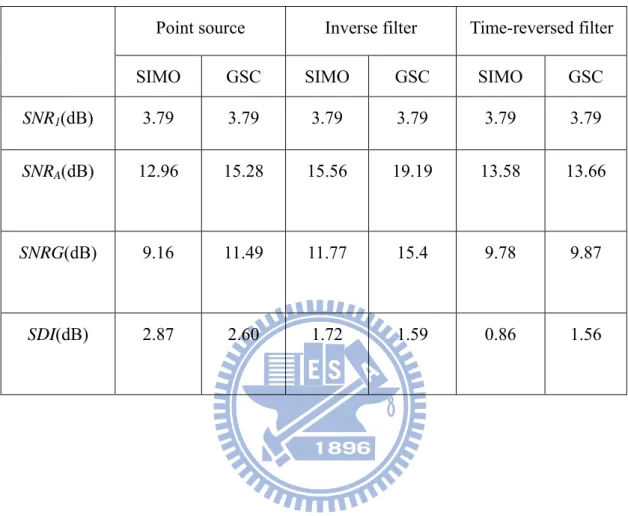
TABLE II The performance of the six proposed algorithms in terms of the objective measures.

Point source Inverse filter Time-reversed filter

SIMO GSC SIMO GSC SIMO GSC

SNR1(dB) 3.79 3.79 3.79 3.79 3.79 3.79

SNRA(dB) 12.96 15.28 15.56 19.19 13.58 13.66

SNRG(dB) 9.16 11.49 11.77 15.4 9.78 9.87

TABLE III. The MANOVA output of the listening test of the six proposed algorithms. Cases with significance value p below 0.05 indicate that statistically significant difference exists among all methods.

Significance value p

Noise type SIG BAK OVL

FIG. 1 The block diagram of SIMO-ESIF algorithm. ( ) q ω   H2( )ω qˆ( )ω   ( ) M H ω 1( ) c ω 1( ) p ω 1( ) H ω   2( ) c ω 2( ) p ω ( ) M p ω c_M( )ω

FIG. 2 The block diagram of the generalized sidelobe canceller. Microphones

( )

0 x k

( )

1 x k

( )

1 M x ₋ k θ d k

( )

d k

(

−Q

)

( )

0 y k

( )

1 y k

( )

M R y ₋ k

( )

z k FBF: Fixed Beamformer BM: Blocking Matrix MC: Multiple-input Canceller Output

FBF

BM

MC

Q z−

Fixed filter

FIG. 3 The block diagram of GJBF structure.

Adaptive Filter

FBF

BM

MC

Fixed filter Fixed filter Fixed filter Adaptive Filter Adaptive Filter

( )

y k   1 L Z−   ( ) 0 z k

( )

1 z k  

( )

2 z k  

( )

1 x k  

(

( )

o k   f

)

2 x k  

( )

3 x k  

FIG. 4 The block diagram of LAF-LAF structure. Fixed filter LAF FBF BM MC Fixed filter Fixed filter Fixed filter LAF LAF LAF LAF LAF LAF LAF 1 L Z−   y k

( )

 

( )

0 z k  

( )

1 z k

( )

  0 x k  

( )

1 x k   fo k

( )

 

( )

( )

(

k

( )

)

3 x   2 x k  

( )

2 z k  

( )

3 z k   2 L − 2 L   Z − 2 L Z   − 2 L   Z −   Z

FIG. 5 The block diagram of SIMO-ESIF-GSC algorithm. 0 H w ( )k p   +    q( )k   z k( )  ‐  H a w H B    

-60 -40 -20 0 20 40 60 -35 -30 -25 -20 -15 -10 -5

Direction of Arrival (Degrees)

Gai n ( d B ) 500Hz 1000Hz 2000Hz Target Signal FBF Directivity

FIG. 6 The directivity pattern of the SIMO-ESIF-GSC algorithm in difference frequency. (a) Fixed beamformer (FBF).

-60 -40 -20 0 20 40 60 -25 -20 -15 -10 -5 0

Direction of Arrival (Degrees)

Ga in (d B ) 500Hz 1000Hz 2000Hz Target Signal BM Directivity

FIG. 6 The directivity pattern of the SIMO-ESIF-GSC algorithm in difference frequency. (b) Blocking matrix (BM).

-60 -40 -20 0 20 40 60 -38 -36 -34 -32 -30 -28 -26 -24

Direction of Arrival (Degrees)

Ga in (d B ) LAF-LAF GJBF GSC

FIG. 7 The compared beam pattern of the GJBF, LAF-LAF and SIMO-ESIF-GSC algorithm in 500 Hz.

Target source

Microphone array

Noise source

0.2 0.4 0.6 0.8 1 1.2 1.4 1.6 1.8 2 x 104 -0.6 -0.4 -0.2 0 0.2 0.4 0.6 time(sample) A m pl it ude(V ) unprocess PIF GSC-PIF

FIG. 9 The performance of SIMO-ESIF algorithm and SIMO-ESIF-GSC algorithm in three different designed methods. (a) PIF algorithm compared with GSC-PIF algorithm.

0.2 0.4 0.6 0.8 1 1.2 1.4 1.6 1.8 2 x 104 -0.6 -0.4 -0.2 0 0.2 0.4 0.6 time(sample) A m pl it ude(V ) unprocess MIF GSC-MIF

FIG. 9 The performance of SIMO-ESIF algorithm and SIMO-ESIF-GSC algorithm in three different designed methods. (b) MIF algorithm compared with GSC-MIF algorithm.

0.2 0.4 0.6 0.8 1 1.2 1.4 1.6 1.8 2 x 104 -0.6 -0.4 -0.2 0 0.2 0.4 0.6 time(sample) A m pl it ude(V ) unprocess MTR GSC-MTR

FIG. 9 The performance of SIMO-ESIF algorithm and SIMO-ESIF-GSC algorithm in three different designed methods. (c) MTR algorithm compared with GSC-MTR algorithm.

FIG. 10 The comparison of the six proposed algorithms. The results of the listening test are processed by using the MANOVA.