交通監控影片中日夜車流壅塞之分析及評估

(1)

國

立

交

通

大

學

資訊科學與工程研究所

碩

士

論

文

交通監控影片中日夜車流壅塞之分析及評估

Traffic Congestion Classification for Daytime and Nighttime

Surveillance Videos

研究生：蔡立武

指導教授：李素瑛教授

(2)

i

交通監控影片中日夜車流壅塞之分析及評估

研究生:蔡立武

指導教授:李素瑛教授

國立交通大學資訊科學與工程研究所

摘要

近年來，各國致力於智慧型運輸系統的開發，以期能透過即時的交通訊息傳輸與整合來提升交通運輸品質。對於一般大眾，若能從中獲得即時的交通壅塞資訊則是更加的實用。目前，由攝影機所構成的交通監控系統已成為交通訊息偵測的主流，然而大部分的研究僅限於監控影片中交通事件的自動分析，例如交通事故與違規事件，但這無法幫助我們得知當下車流的壅塞情形。所以，處理監控影片以提供民眾最即時的交通壅塞資訊是迫切需要的。在本論文中，我們提出了一個適用於白天與晚上交通監控影片的壅塞程度評估系統能將壅塞程度分為五個等級。想要從影片中評估交通壅塞程度，視訊處理的技巧與相關的知識是不可或缺的。對於白天的影片，我們利用背景相減法來找出道路上的車子，而在晚上的影片中，則是透過車頭燈的偵測來找出車子的位置。當車子擷取出來之後，我們使用虛擬的偵測器來蒐集交通訊息，藉此即時地評估所偵測到的車流壅塞程度。除此之外，我們也針對道路偵測、車流方向判斷與車道偵測等問題提出解決方法，以提升整個系統的即時性與完整性。最後，我們利用高速公路上的交通監控影片來驗證我們所提出系統的性能，並獲得了令人滿意的結果。

(3)

ii

關鍵字：交通壅塞、車道偵測、夜間監控、車燈偵測、虛擬偵測器、智慧型運輸系統

(4)

iii

Traffic Congestion Evaluation for Daytime and Nighttime

Surveillance Videos

Student: Li-Wu Tsai Advisor: Prof. Suh-Yin Lee

Institute of Computer Science and Engineering National Chiao Tung University

Abstract

In recent years, intelligent transportation system is developed to promote the quality of the traffic transportation. In general, concerns of the traffic control center are traffic management, vehicle control, and traffic safety. However, they are not the issues that people concern most. Instead, the situation of traffic congestion is much more useful for the public. In addition, traffic surveillance systems have been widely used for monitoring the roadways. There have been many researches on video analysis of traffic activities such as traffic accidents and violations, but these researches still cannot help people get to know the traffic congestion situation. Therefore, we intend to develop techniques to process traffic surveillance videos for providing people with instant traffic congestion information. In this thesis, a traffic congestion classification framework is proposed for identifying the traffic congestion levels in daytime and nighttime surveillance videos. The degrees of traffic congestion are classified into five levels: jam, heavy, medium, mild and low.

In order to analyze the traffic congestion levels from videos, image processing techniques and the knowledge of classification are indispensable. In the proposed

(5)

iv

framework, moving vehicles are extracted by background subtraction during the day and by headlight detection at night. Afterward, virtual detectors and virtual detection line are utilized to evaluate and classify the traffic congestion levels in daytime and nighttime surveillance videos, respectively. Moreover, methods of bidirectional roadway detection and lane detection are proposed to extract the consistent features of roadway for the requirements of real-time response and robustness of the frameworks.

In the experiments, we use real freeway surveillance videos captured at day and night to demonstrate the performances on accuracy and computation. Satisfactory experimental results validate the effectiveness of the proposed framework.

Keywords: traffic congestion, roadway detection, lane detection, nighttime, headlight

(6)

v

Acknowledgement

I greatly appreciate the patient guidance, the encouragement, and valuable comments of my advisor, Porf. Suh-Yin Lee. Without her graceful advices and help, I cannot complete this thesis. Besides, I want to extend my thanks to my friends and all members in the Information System laboratory, Yee-Choy Chean, Hui-Zhen Gu, Chien-Peng Ho, Hua-Tsung Chen especially. They gave me a lot of suggestions and shared their experiences.

Finally, I would like to express my appreciation to my dear family for their supports. This thesis is dedicated to them.

(7)

vi

List of Figures

Figure 1. Captured frames in five congestion levels ... 2

Figure 2. Lane markings with different shapes and colors on the roadway ... 6

Figure 3. Three roadway types ... 7

Figure 4. Cast Shadow and self shadow ... 10

Figure 5. Generation procedure of time-spatial image... 13

Figure 6. Overview of the proposed framework ... 16

Figure 7. A traffic scene of a bidirectional roadway consisting of six lanes. ... 20

Figure 8. An example of roadway detection ... 23

Figure 9. An example of bidirectional roadway analysis ... 26

Figure 10. MBSAS processing on the history of the central points of vehicles ... 29

Figure 11. Results of virtual detectors installation on a bidirectional roadway ... 30

Figure 12. Gradient images of foreground and its relevant background... 35

Figure 13. Result of shadow elimination by using gradient feature ... 36

Figure 14. Operators of Sobel filter ... 36

Figure 15. Determination of traffic congestion thresholds for NCD ... 41

Figure 16. Headlights with different color lights ... 43

Figure 17. Results of bright region detection. ... 44

Figure 18. The parameters of height relationship for two headlights ... 48

Figure 19. The parameters of edge relationship of two headlights ... 48

Figure 20. Experimental results of roadway detection... 54

Figure 21. Experimental results of bidirectional roadway analysis ... 56

Figure 22. Experimental results of virtual detector installation ... 58

Figure 23. Classification accuracy in five levels by different parameters (NCD). ... 61

Figure 24. Classification accuracy in five levels by different parameters (SVM). ... 63

Figure 25. Experimental results of headlight detection ... 67

(10)

ix

List of Tables

Table 1. Luminance and color variation from the center to boundary of headlights. . 43 Table 2. Distribution of experimental daytime surveillance video data. ... 59 Table 3. Comparison of classification performance with different features (NCD). .. 61 Table 4. Daytime traffic congestion classification results by using Congday (NCD). . 62

Table 5. Daytime traffic congestion classification results by using Dens (NCD). ... 62 Table 6. Daytime traffic congestion classification results by using Sp (NCD). ... 62 Table 7. Comparison of classification performance with different features (SVM). .. 63 Table 8. Daytime traffic congestion classification results by Congday (SVM). ... 64

Table 9. Daytime traffic congestion classification results by Dens (SVM). ... 64 Table 10. Daytime traffic congestion classification results by Sp (SVM). ... 64 Table 11. Time for processing one frame in five congestion levels in daytime video. 65 Table 12. Distribution of experimental nighttime surveillance video data. ... 70 Table 13. Nighttime traffic congestion classification results by Congnight (NCD). ... 71

Table 14. Nighttime traffic congestion classification results by Congnight (SVM). ... 72

Table 15. Time for processing one frame in five congestion levels in nighttime video.

(11)

1

Chapter 1. Introduction

Traffic surveillance systems have been widely used for monitoring roadways in recent years. Unfortunately, the repository of the captured videos is so large that it is almost impossible to manually understand the contents of the videos. In fact, it is useful to utilize these traffic video data which can be processed to extract abundant traffic information for real-time intelligent transportation applications. Therefore, plenty of researches have been focused on automatic traffic events analysis such as traffic accidents, violation, and congestion. In this thesis, we investigate the event that the public concern most: roadway traffic congestion.

In the past, when traffic jams occurred, the police or drivers would inform the traffic control centers, and people detoured to avoid the traffic jams after radio station broadcasted that information. Nowadays, a variety of sensors such as loop detector, infrared detector, and Closed Circuit Television camera are used to gather the instant traffic information in traffic control system. However, the cameras are the particular devices that not only can observe the traffic situation but also record all events that happen on roadways all the time, which provides us with more plentiful traffic information. Moreover, due to the advantage of non-invasive installation, the cameras have distributed over all freeways and the main roadways in metropolises. Thus, it facilitates the possibility of the establishment of the complete traffic information. If a traffic surveillance system can automatically analyze the level of traffic congestion from traffic surveillance videos, the congestion message can be immediately provided for the public. Moreover, with the rapid development of intelligent mobile devices such as smart phone and personal digital assistant, drivers can earlier get traffic information and recommended alternate routes for avoiding traffic jam.

(12)

2

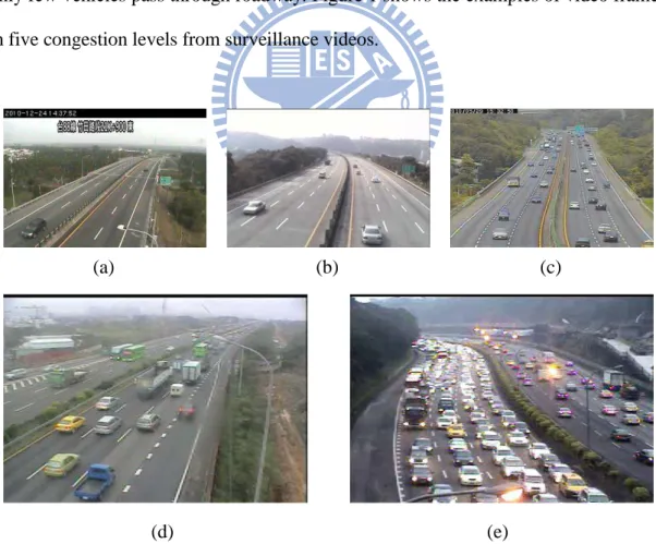
Aiming at the benefits arising from integration of video analysis technique and intelligent mobile devices, real-time classifying the traffic congestion in daytime and nighttime surveillance videos is the goal we are going to achieve in this thesis. The traffic congestion is classified into five levels: jam, heavy, medium, mild, and low. Jam is the situation that the vehicles fully occupy the roadways and almost all of the vehicles move slowly or completely stop. Heavy indicates that most of the vehicles on the roadway run slowly but seldom stop. In medium level, the difference from aforementioned levels is that all vehicles can move smoothly, and there still are many vehicles moving on the roadway. Mild means that the number of vehicles is much less than that in medium level and the vehicles move at normal speed. Low denotes that only few vehicles pass through roadway. Figure 1 shows the examples of video frames in five congestion levels from surveillance videos.

(a) (b) (c)

(d) (e)

Figure 1. Captured frames in five congestion levels. (a) Low. (b) Mild. (c) Medium. (d)

(13)

3

In order to analyze the traffic information from video, image processing techniques and knowledge of classification are essential. In general, procedure of analyzing video comprises selection of the region of interest, vehicle detection, vehicle tracking, and activity analysis. Nevertheless, in most of the existing works, a fundamental problem is that the performance of video analysis may not be stable with the varied environments. For example, a large number of vehicles may lead vehicle occlusion and cause the failures of vehicle segmentation. Moreover, vehicles which have similar features such as color, shape, texture, and moving direction increase the difficulty in vehicle tracking. On the other hand, a critical issue is that image processing is always time-consuming. For the requirement of real-time response, developing efficient frameworks and algorithms of video analysis is an important and inevitable challenge. Consequently, how to quickly and accurately evaluate the traffic congestion from traffic surveillance videos is the core problem in our work.

In this thesis, we propose a real-time traffic congestion classification framework which consists of daytime and nighttime modules to automatically process the daytime and nighttime surveillance videos for identifying the traffic congestion levels. For daytime surveillance videos, the moving vehicles on the roadway are extracted by background subtraction and shadow elimination technique. Afterward the extracted vehicles are used to calculate the important traffic parameters including traffic flow, traffic speed, and traffic density. Then the traffic parameters are utilized to evaluate and classify traffic congestion levels. For nighttime surveillance videos, the moving vehicles are detected by extracting and grouping the headlight candidates. Subsequently a virtual detection line is utilized for evaluating the traffic congestion levels. Finally, we examine the proposed framework on real freeway surveillance videos captured at day and night data to demonstrate the accuracy and real-time response of traffic congestion classification.

(14)

4

The rest of this paper is organized as follow. Some related works on daytime and nighttime video processing are reviewed in Chapter 2. In Chapter 3, we introduce the proposed framework of traffic congestion classification. After that, we present the daytime module that includes initialization procedure, vehicle detection and traffic congestion classification in Chapter 4. In Chapter 5, the module of nighttime traffic congestion classification which is composed of headlight extraction, vehicle detection and traffic congestion classification is described. The experimental results of daytime module and nighttime module are shown and discussed in Chapter 6. In Chapter 7, we conclude this thesis and discuss the future works.

(15)

5

Chapter 2. Related Work

In this chapter, we review the previous research works on daytime surveillance and nighttime surveillance video processing. The details are described as follows.

2.1 Related work on Daytime Surveillance

In the past, plenty of works related to daytime traffic surveillance had been proposed [1]. In the following sections, some methods of roadway detection, object detection, shadow elimination, and traffic surveillance video analysis are introduced.

2.1.1 Roadway Detection

In traffic surveillance videos, roadway is the only region that we are interested in, and the rest regions in video frames are worthless. Therefore, finding out the region in advance reduces the computation of video processing and decreases errors caused by moving objects outside the roadway. In addition, discovering a center line of bidirectional roadway is helpful to monitor respective traffic flows in two directions.

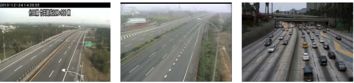
Li and Chen [2] propose an algorithm to detect the lane boundaries of roadway by using Multi-resolution Hough Transform [3] without a priori knowledge of road geometry or training data. Then the region between the lane boundaries is regarded as roadway region. Lai et al. [4] put forward a method to detect multiple lanes from a traffic scene by using lane marking information and orientation. However, there are many types of lane markings like solid line, double solid line, and dotted line on different kinds of roadway as shown in Figure 2. Therefore, finding the correct lane

(16)

6

Figure 2. Lane markings with different shapes and colors on the roadway.

markings is not a simple task. Furthermore, the lane markings of the roadway are not always visible in some cases. Hence, there are other researches on roadway detection without lane marking information.

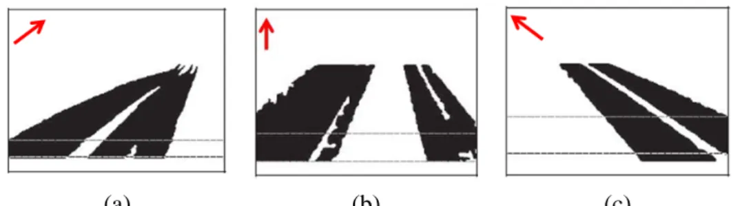
Stewart et al. [5] present an automatic lane finding algorithm based on detecting a region with significant changes. The roadway region in a traffic scene is generated by accumulating the differences between two consecutive frames after removing noises and sudden changes in brightness. However, a limitation of their algorithm is that the roadway must be parallel to the direction of camera shooting. Afterwards, Pumrin and Dailey [6] improve the algorithm to detect the roadway region from a variety of camera angles. For generating a roadway region mask, a hundred frames of moving edge images are accumulated and then holes are filled with a convex hull algorithm. In addition, two successive activity region masks generated from two successive sets of hundred frames are compared to detect the camera’s motion. In [7], Lee and Ran put forward a method to detect bidirectional roadway by accumulating moving parts in a difference image between two consecutive frames and find a center line to separate the roadway into two parts with different directions. Nevertheless, their methods are affected by unbalanced traffic flow in different lanes and constrained by three roadway types. As shown in Figure 3, the roadway may extend to a) bottom-right, b) bottom-mid, c) bottom-left. Moreover, a clear gap must exist between the two respective parts in two directions for center line estimation.

(17)

7

(a) (b) (c)

Figure 3. Three roadway types. (a) Bottom-right. (b) Bottom-mid. (c) Bottom-left.

Therefore, in order to conquer the drawbacks in previous works, the roadway detection and bidirectional roadway analysis without any lane marking information and a limitation of specific roadway types are proposed in our framework.

2.1.2 Object Detection

Detecting the moving objects is an important and useful technique for video understanding. Thus, many techniques are developed and can be classified into four categories: background subtraction, segmentation, pointer detectors and supervised learning [8]. Among the four categories, background subtraction is a widely used method for detecting moving objects in videos captured by static cameras. The rationale of the method is to detect the moving objects from the significant differences between the current frame and a reference frame, often called “background image” or “background model”. However, this method suffers from the background varying. Thus, the background image must be a representation of the scene without moving objects and keeps regularly updated so as to adapt to the changing geometry setting and luminance condition [9]. Since roadway surface is even and smooth in most cases and traffic surveillance is stable without camera motion, we employ background subtraction technique for the advantages of integrity of foreground and low computation complexity in extracting the moving vehicles on the roadway.

(18)

8

A variety of algorithms and techniques for performing background subtraction have been developed to detect vehicles. Averaging [10] and finding the median values [11] of a sequence of frames are the most basic ways to construct the background image in the past. Subsequently, Chen et al. [12] put forward a background image construction by calculating the frequency of pixel intensity value at training period. The frequency ratios of intensity values for each pixel at same position in frames are calculated and the intensity values with biggest ratio are incorporated to model a background image. Then, the background image is updated by repeating initialization operation. However, the aforementioned methods are fast but memory consuming and do not provide explicit methods to choose a threshold for segmenting out the foreground. Hence, Wren et al. [13] propose a running Gaussian average background model which fits a Gaussian probability density function on the latest n values of a pixel location for each pixel in a frame. In addition to the low memory requirement, that the threshold is determined automatically by standard deviation is the most significant improvement.

In some conditions, different objects are likely to appear at a same location over time. Therefore, some researches are proposed to deal with multiple modal background distributions. Stauffer and Grimson [14] raise a case for a multi-valued background model that is capable of coping with multiple background objects. The recent history of each pixel, called pixel process, is modeled by a mixture of K Gaussian distributions, and each pixel is classified into foreground or background according to whether the pixel matches one distribution of its pixel process. In a highly volatile environment, Elgammal et al. [15] propose a method to model the background by a non-parametric model based on kernel density estimation on the last

n values. The method rapidly forgets the past and concentrates on recent observation

(19)

9

which requires great amount of data to be accurate and unbiased.

On the other hand, traditional background subtraction approaches model only temporal variation of each pixel. However, there is also spatial variation in real world due to dynamic background such as waving trees and camera jitters, which causes a significant performance degradation of traditional methods. A novel spatial-temporal nonparametric background subtraction approach is proposed by Zhang et al. [16] to handle dynamic background by modeling the spatial and temporal variations at the same time. Moreover, other various background subtraction methods suitable for different environments have been reviewed and discussed in [1, 16, 17].

2.1.3 Shadow Elimination

When we detect the moving objects in the outdoor images, shadows are often extracted with the objects. Also, separate objects may be connected through shadows. Both conditions always cause failure in object detection. However, separating the moving objects from shadows is not a trivial task. As shown in Figure 4, shadows can be generallycategorizedcast shadow and self shadow [18]. Referring to Figure 4, the self shadow is a portion of the object not illuminated by the light source. The cast shadow lying beside the object does not belong to the object. For object detection and many applications, cast shadow is undesired and should be eliminated, while self shadow is a part of the object and need to be preserved. However, cast shadow and self shadow are similar in intensity. Thus, how to distinguish between them becomes a serious challenge. Moreover, if an object has intensity close to its shadows, shadow elimination is extremely difficult. Sometimes even though object and shadows can be separated, object shape is often incomplete due to imprecise shadow removal.

(20)

10

Figure 4. Cast Shadow and self shadow.[18]

Confronting these knotty problems, various methods for shadow elimination have been proposed for suppression of cast shadow in recent years. The intensity, color and texture are the most remarkable features of shadow. Because the distribution of intensity within a shadow is not uniform in real environments, Wang et al. [18] develop a method to estimate attributes of shadow by sampling points on edges of cast shadow and remove the shadow by the attributes. Afterwards, a process is executed to recover the object shape on the basis of information of object edges and attributes of shadow for avoiding over-elimination. Song et al. [19] remove the shadow in good use of the different properties between shadows and objects based on the RGB chroma model. Liu [20] introduces a method which uses gradient feature to eliminate shadow based on the observation that shadow region presents the same textual characteristics as in the corresponding background image.

Based on the prior knowledge, Yoneyama et al. [21] simplify 3D solid cuboids model to a 2D joint vehicle-shadow model for eliminating cast shadow. Six types of vehicle-shadow models are employed to match the extracted vehicle by utilizing luminance of shadow for differentiating the vehicle and shadow. Besides, Chien et al. [22] remove the shadow by a mathematical analysis model. Different from the methods mentioned above, Hsieh et al. [23] use lane geometries as an important cue to help eliminate all undesirable shadows even though the intensity, color and texture of vehicles are similar to cast shadow.

(21)

11

A summary of general observations with respect to cast shadow and background in roadway scene is given by Xie et al. [24] : (1) Pixels of cast shadow fall on the same surface as the background; (2) Cast shadow pixels are darker than their background in all three color channels; (3) Background is mostly roadway surface which is often monochrome in traffic scene. As a result, the values of hue channel are small in the cast shadow region; (4) The edge pixels of the cast shadow are significantly less than that of the vehicle.

2.1.4 Traffic Surveillance Video Analysis

For analyzing the content of video, the trajectories of moving objects can provide much information, and object tracking is an important and unavoidable way to extract the trajectories. Take traffic surveillance videos for example, if we intend to realize the action of moving vehicles, we have to analyze how the vehicles move. That is, we must track vehicles during the traffic monitoring in order to obtain their trajectories. Generally, tracking methods can be classified into two categories. One category estimates motions of moving objects and minimizes the error function to track objects. Another category calculates the similarities between current objects and previous objects and maximizes the similarity measures to track the objects. A variety of object tracking methods developed in past decades are reviewed in [8].

In traffic surveillance videos, a traditional approach of moving vehicles tracking is to model the moving object properties such as position, velocity and acceleration. Measurements usually include the object positions in the frame, which is obtained by an object detection algorithm. In particular, Kalman filter [25] and particle filter [26] are popularly used in many research works. However, in practical applications, it is difficult to track all vehicles on the roadway. For examples, if the viewpoint of a

(22)

12

camera is low or there are plenty of vehicles on the roadway, the vehicle occlusion problem results in failing to extract and track correct individual vehicles. Moreover, that the effective resolution of perspective is reduced in a frame makes insufficient features of vehicles for object tracking. Even though many researches on occlusion problem have been proposed, the complexity of vehicle tracking is surged and accuracy of vehicle tracking is sagged while a great number of occluded vehicles need to be tracked at one time.

Along with the trajectories of vehicles are extracted, numerous works deal with vehicle activity analysis. The features such as size, speed, and moving direction of vehicles are helpful to understand the situation of traffic flow in the surveillance videos [2]. Generally, more complicated events are mostly detected with machine learning algorithms. In [27], the issue of event detection in time series data is addressed using neural network. In [28], Hidden Markov Models are used to form the basis of activity recognition and anomaly detection.

For the purpose of traffic flow analysis, the usage of virtual line detectors without tracking all vehicles on the roadway was developed in [29-33]. In [29], the authors present an approach to evaluate traffic-flow parameters under urban road environment. Virtual line based time-spatial image as shown in Figure 5 is used for vehicle counting. The vehicles are extracted from the time-spatial image after edge detection and morphological operation. In [30], the time-spatial image is processed to evaluate the traffic congestion level. However, these methods do not work well in the frames with low contrast, small vehicle blocks, and irregular driving behaviors. Afterwards, the virtual line group methods are proposed as an improvement in [32, 33]. Actually, virtual line based algorithms are more suitable to analyze the traffic flow while there are a large number of vehicles for real-time performance.

(23)

13

Figure 5. Generation procedure of time-spatial image.[29] (a) A frame sequence. (b)

Time-spatial image generated by virtual line iteration.

2.2 Related Work on Nighttime Surveillance

Due to low illumination, understanding the activities in nighttime videos becomes more difficult than in daytime for the frames captured from a camera have lower contrast and higher noise than their corresponding daytime frames. Thus, nighttime video analysis is still quite a challenging task up to the present. In this section, we will review some studies on nighttime surveillance video processing.

2.2.1 Nighttime Image Enhancement

In order to solve the low contrast problem, some researches focus on nighttime image enhancement. Histogram equalization is a commonly used method for image enhancement in luminance of image. Hence, Sayed et al. [34] propose an efficient algorithm that modifies traditional histogram equalization to maintain the color information of the original nighttime image. Each color channel is enhanced separately by multiplying the ratio of enhanced luminance to original luminance.

Nevertheless, the performance of enhancement is limited due to the detailed information of nighttime frames has been lost. Therefore, Cai et al. [35] combine

(24)

14

daytime image and nighttime image together based on the object extraction technique. The low quality static parts of a nighttime image can be replaced by the high quality counterpoint in the daytime image. However, if errors occur in object extraction, unnatural mixture images may be generated. In [36], authors can produce natural-appearing enhanced images that do not appear to be fake. The image is decomposed into luminance and reflectance components, and only the luminance of the image is modified by referring to daytime background.

2.2.2 Object Detection and Tracking

As mentioned in previous section, due to the low contrast problem in nighttime video, detecting moving objects from the dark scenes becomes difficult. Even though the nighttime image enhancement technique improves appearance of nighttime images, object detection based on background subtraction is quite arduous. Hence, in [37], the authors put forward an algorithm that is based on contrast analysis to detect moving objects. They use the local contrast change over time to detect potential moving objects, which is called Salient Contrast Change (SCC). Then motion prediction and spatial nearest neighbor data association are used to suppress false alarm. Wang et al. [38] propose a model based on SCC feature which applies learning process to strength adaptability and analyze trajectories to improve the effectiveness of detection.

For nighttime traffic surveillance, Kostia Robert [39] presents a framework to detect multiple vehicles at night by headlight detection. He adopts HSV color model and uses the ratio of value to saturation (V/S) with white top-hat transform operation to obtain the bright blobs as headlights. Then the blobs are analyzed to generate hypothesis of vehicles. In [40], in order to extract headlights, a bright object

(25)

15

segmentation process based on automatic multilevel histogram thresholding is applied on the nighttime scenes of roadway.

In the case of object tracking, in general, conventional tracking methods such as model-based, appearance-based, and feature-based cannot work well at night due to insufficient detailed information. Thus, an appropriate solution is to track vehicles by using position and velocity. In [39], the vehicles are tracked over frames by using a Kalman filter associated with a reasoning module. Also the tracking processing in [37, 40] are based on these features.

(26)

16

Chapter 3. Proposed Framework Overview

In this chapter, we make an introduction of the proposed traffic congestion classification framework. The framework, which consists of daytime module and nighttime module, is able to classify the traffic congestion in traffic surveillance videos captured during day and night into five levels.

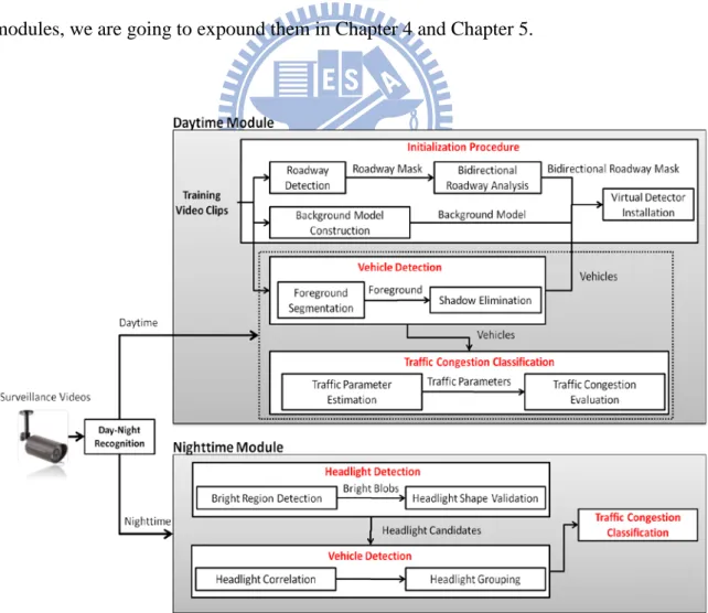
As shown in Figure 6, in the framework, a video clip is firstly determined whether it is captured at day or at night, and the corresponding modules are applied on the video according to the capturing time. The brief descriptions of the two modules are described in the following sections. As for the details of each component in the modules, we are going to expound them in Chapter 4 and Chapter 5.

(27)

17

3.1 Daytime Traffic Congestion Classification

The goal of the daytime module is to automatically analyze the level of traffic congestion in daytime surveillance videos. In general, vehicle detection and tracking are inevitable ways to realize the content of traffic surveillance videos. However, some troublesome factors such as a great number of moving vehicles with serious vehicle occlusion not only increase the difficulty in detecting and tracking the moving vehicles, but also lower the efficiency of video processing. Therefore, in order to understand the traffic condition, we adopt a novel strategy that uses virtual detectors to simplify the processes of vehicle detection and tracking. Based on this strategy, it is unnecessary to extract and track all moving vehicles on the roadway for analyzing the surveillance videos. Furthermore, we also put forward two methods to detect the roadway region and distinguish the moving direction of roadway to enhance efficiency and robustness of the module. As shown in Figure 6, the module contains three major parts: initialization procedure, vehicle detection, and traffic congestion classification.

Initialization procedure is performed at the beginning of traffic monitoring in order to obtain the consistent characteristics of roadway including the region and moving direction of roadway, positions of virtual detectors and background model. As Figure 6 illustrates, we first extract the roadway region because only monitoring the area that we are interested in is helpful for the efficiency and accuracy enhancement. Second, bidirectional roadway analysis is applied on the roadway region in order to monitor both directions of roadway at the same time. Moreover, the background model is also constructed along with the above processes, and the model is updated with incoming frames over time. Finally, virtual detectors are automatically installed on each lane of roadway for gathering traffic flow information. In addition, since

(28)

18

initialization procedure executes only once in advance, there is no requirement of strict real-time response.

Vehicle detection is to extract the moving vehicles from videos. We use background model to segment the foreground image and eliminate the shadow by using two characteristics of shadow: edge and color reflectance. Next, connected component analysis clusters all adjacent pixels in foreground image as isolated moving vehicles. Because the virtual detectors are adopted to gather traffic information in the module, only the moving vehicles that pass through the virtual detectors are need to be detected and tracked. In this way, the efficiency of video processing is promoted a lot.

In traffic congestion classification, the virtual detectors estimate three traffic parameters: traffic flow, traffic speed and traffic density by tracking the moving vehicles that pass through the detectors. For a sequence of moving vehicles over a period of time, the parameters are calculated and utilized to evaluate traffic congestion degree. Finally, we use classifier to make an accurate classification of traffic congestion levels. With bidirectional analysis, the proposed module is capable of analyzing both directions of roadway at the same time.

3.2 Nighttime Traffic Congestion Classification

The proposed night module is able to classify the congestion level of traffic flow in nighttime surveillance videos. In order to understand the content of traffic surveillance videos, in general, vehicle detection is usually the first step. However, some tough factors such as poor visibility and higher noise increase difficulty in detecting the moving vehicles under nighttime condition. Especially, typical daytime surveillance framework based on background subtraction cannot work at night due to the low contrast foreground objects against the background, which is an obstacle to

(29)

19

vehicle detection at night. On the other hand, less color and texture information may lower the ability of vehicle tracking to distinguish between different moving vehicles. To overcome these limitations, an appropriate solution for vehicle detection is to find headlight that is a salient feature to all vehicles at night. Hence, in the nighttime module, headlight detection and grouping technique are developed to extract the moving vehicles on the roadway. In addition, we abandon vehicle tracking appoaches for analyzing traffic congestion due to the reasons below. Headlights of all vehicles are similar to each other. The large number of vehicles in crowded situation causes high complexity in vehicle tracking. Therefore, a virtual detection line is utilized to evaluate traffic congestion degree for avoiding errors caused by vehicle tracking and enhancing the execution efficiency.

The module includes three stages: headlight extraction, vehicle detection, and traffic congestion classification. Headlight extraction is performed at the beginning of each frame processing to recognize the circle-shaped bright blobs that is most similar to headlight. At vehicle detection stage, correlation of two headlights is calculated by using three features: width, height and edge relationships between them. After that, the values of correlation are used in our headlights grouping mechanism to detect the moving vehicles. For a sequence of video frames, traffic congestion is evaluated when the moving vehicles pass through a virtual detection line. A virtual detection line is a virtual horizontal line that crosses a roadway and is employed to gather the traffic information. In other words, only the headlights that touch the virtual detection line need to be extracted and grouped. Then, the possible mistakes from headlights grouping are decreased and the efficiency for video processing is raised.

(30)

20

Chapter 4. Daytime Traffic Congestion Classification

In this chapter, we describe the daytime traffic congestion classification module. The module contains initialization procedure, vehicle detection and traffic congestion classification as presented in the following sections.

4.1 Initialization Procedure

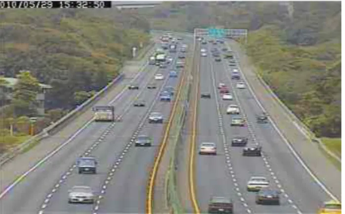
Initialization procedure is executed at the beginning of traffic monitoring and utilizes training video data to obtain the consistent characteristics of roadway including the region and moving direction of roadway, positions of virtual detectors and background model. In this section, we present our approaches of roadway detection, bidirectional roadway analysis and virtual detector installation in details. To make it easier to understand the proposed approaches, a traffic scene is used to be an example for demonstration as shown in Figure 7.

(31)

21

4.1.1 Roadway Detection

Some peculiar phenomena exist in the traffic surveillance videos. For example, shaking trees outside the roadway causes frequent motions over time. We realize two important facts by observation. First, all moving pixels outside the roadway must not belong to any vehicles. Second, surface of roadway is much stable than other regions outside the roadway. In other words, most moving pixels on roadway are a part of vehicles and actually need to process. Hence, an efficient way to remove most of useless pixels is to detect a region of roadway in advance, and then we can focus the further video processing only on the roadway region. This approach not only avoids unnecessary mistakes, but also reduces the time-consuming video processing.

In our framework, we develop a process to accomplish the roadway detection based on the concept that roadway is a region where most movements occur because of vehicle motion. Therefore, we calculate the differences between two consecutive frames to detect the movements and accumulate the movements to obtain the position and shape of roadway. The difference image D is defined as follows:

   − > + = − − otherwise , 0 | ) , ( ) , ( | if , 1 ) , ( ) , ( 1 1 M t t t t F x y F x y th y x D y x D ₍₁₎

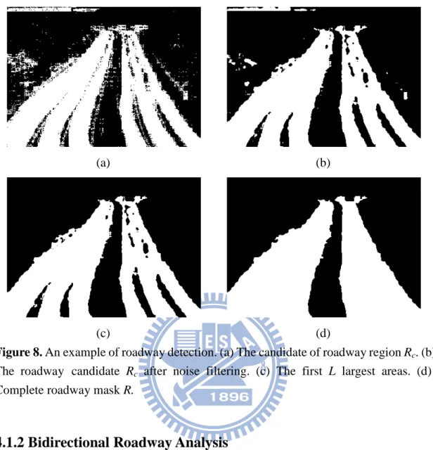
where Ft(x,y) denotes the current frame t and thM is the pre-defined threshold for identifying the pixels with movements. After accumulation of movements for a sequence of frames, the pixels that have a value in difference image D larger than 0 are regarded as a roadway candidate Rc for the roadway region. The result of the example is shown as Figure 8(a) and the white pixels are the pixels of Rc.

   > = otherwise , 0 0 ) , ( if , 1 ) , (x y D x y Rc (2)

(32)

22

Then, we discover that some fragmentary movements outside the roadway are also detected because of the shaking trees. In order to eliminate the fragmentary movements, the pixels which satisfy the following noise filtering equation are removed from Rc_:

∑ ∑

+ − = + − = < + p x p x i p y p y j R c i j th R p 1) (, ) 2 ( 1 2 (3)

where p control the size of filter and thR is a threshold determined by the characteristic of roadway. Afterward, we employ connected component analysis on Rc as shown Figure 8(b) to extract all isolated connected areas and sort the isolated connected areas in descending order according to their size from S1 to Sn, where n is the number of isolated connected areas. Then choose the first L largest areas as the roadway region.

R r i i r T S S L=

∑

> =1 min arg (4)

where r is a value ranging from 1 to n, S is the summation of S1 to Sn and TR is a measure to maximize the number of areas that should be accounted for the roadway. This operation reserves the main areas of roadway as shown in Figure 8(c). Some small but not fragmentary noises are eliminated successfully. Finally, using Closing morphological operation to fill out the holes and a hole-filling algorithm to obtain the complete roadway mask R as shown in Figure 8(d).

(33)

23

(a) (b)

(c) (d)

Figure 8. An example of roadway detection. (a) The candidate of roadway region Rc. (b) The roadway candidate Rc after noise filtering. (c) The first L largest areas. (d) Complete roadway mask R.

4.1.2 Bidirectional Roadway Analysis

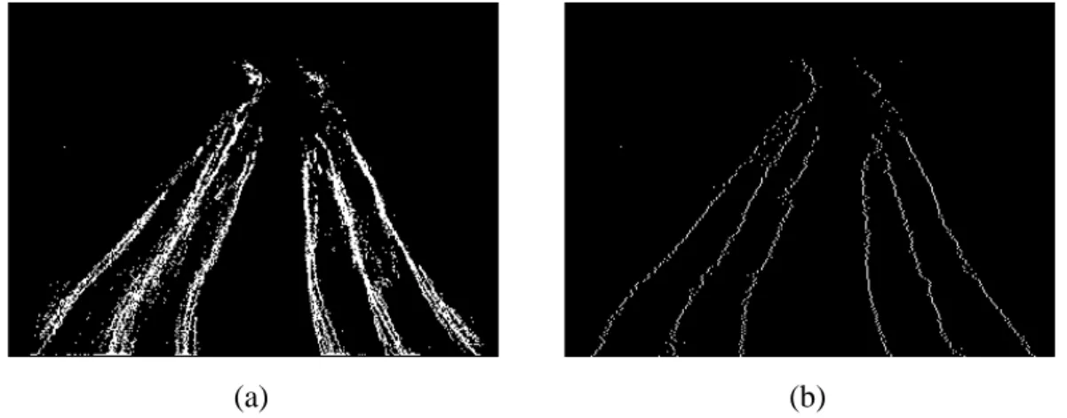
Most surveillance cameras capture a video at a specified angle and range that contains multiple lanes of traffic in both directions. The bidirectional roadway analysis can be applied to monitor traffic flow for both directions individually. During the period of movement accumulation in roadway detection, the occurrence of movements means some motions appear at the same time. Accumulation of those motions is able to approximately reveal the moving direction of roadway. Hence, we estimate and accumulate the motion vectors for those pixels that have movements in roadway detection. A Motion Vector image MV is defined as follows:

(34)

24     < − > + = − 0 ) , ( , 1 0 ) , ( , 1 ) , ( ) , ( 1 y x m y x m y x MV y x MV _t y t y t t (5)

where mt_y(x,y) denotes the motion vector [41] in y-axis between frame t and t-1. The method to estimate motion vector is described in Algorithm 4.1. Since bidirectional roadway contains two kinds of directions, DOWN and UP, in most cases, the motion vectors in y-axis are only considered. After accumulation of the motion vectors, the Motion Vector image is simplified into a Motion image M:

   < > = 0 ) , ( , UP 0 ) , ( , DOWN ) , ( y x MV y x MV y x M (6)

As shown in Figure 9(a), the white pixels denote the DOWN and the gray pixels denote UP. In order to separate the roadway into two respective parts in different directions, a center line of the roadway for separating the motions should be calculated. A motion classification method is used to obtain this center line. First, the positions of both directions need to be decided by the average x-position of two kinds of motions.

∑

∈ = = R y x DOWN DOWN x M x y N X ) , ( DOWN ) , ( if , 1 (7)

∑

∈ = = R y x UP UP x M x y N X ) , ( UP ) , ( if , 1 (8)

where NDOWN and NUP are the number of pixels of motion DOWN and UP in motion image, respectively. If XDOWN is smaller than XUP, the moving direction of the left side of roadway is DOWN and the right side is UP. Otherwise, the left side is UP and the right side is DOWN.

Then, a center line CL for separating bidirectional roadway is evaluated by rotating a separator line SL. As illustrated in Figure 9(b), each pixel at the top

(35)

25

boundary of roadway region is regarded as a core for SL rotation, and the SL rotates from left boundary to right boundary of roadway mask for each core. For each rotation, we evaluate the separation degree SD of motion classification that bases on the SL. The smaller the SD is, the better the motion classification is. The SL with minimum SD is the actual center line CL of the roadway.

In the SD evaluation, the ratios of error and recall for motion classification are considered at the same time. From the result in the first step, we can know what the well-classified pixels are and what the mis-classified pixels are. For instance, if the left side of roadway is DOWN (XDOWN < XUP), the pixels of motion DOWN in the left side of SL are well-classified and the pixels of motion UP in the left side of SL are mis-classified. Therefore, the error ratio of left side eleft is defined as the ratio between the number of motion UP pixels and the number of total pixels in the left side of SL. The recall ratio of left side rleft is defined as the ratio between the number of motion DOWN pixels and the number of total DOWN pixels in whole roadway mask. Analogously, the rationale is the same for the right side. Separation degree SD is defined as follow: right left right left

r

e

SD

+

=

(9)

where eleft is the error ratio for classification in the left side of SL, eright is the error ratio for classification in the right side of SL, rleft is the recall ratio for classification in the left side of SL, and rright is the recall ratio for classification in the left side of SL. According to the center line CL, the roadway mask is divided into two parts as a bidirectional roadway mask. An example of the center line evaluation and bidirectional roadway mask are shown in Figure 9(c) and Figure 9(d).

(36)

26 Algorithm 4.1: Motion Vector Estimation [41]

Input: The position (x, y) of a pixel, current frame Ft, and previous frame Ft-1

Output: The motion vector in y-axis v for the pixel (x, y)

1 for i := - p to p do

2 for j := -q to q do

3 diff = |Ft(x, y) – Ft-1(x+i, y+j)| 4 if diff < mini_diff then

5 mini_diff = diff ; 6 v = j ; 7 end for 8 end for (a) (b) (c) (d)

Figure 9. An example of bidirectional roadway analysis. (a) Motion image M, the

motion of white pixels is DOWN, the motion of gray pixels is UP. (b) The separator line

SL which is represented by a red dotted line rotates between two boundaries to

calculate the separation degree SD for motion classification. (c) The center line CL which has the minimum SD. (d) Bidirectional roadway mask.

(37)

27

4.1.3 Virtual Detector Installation

As discussed in section 2.1.4, we realize that vehicle tracking technique is not an appropriate way to analyze actions of all vehicles on roadway due to the vehicle occlusion and reduction of effective resolution. Hence, the virtual line based algorithms are the better approaches to analyze the traffic situation for its real-time response and low difficulty in vehicle tracking.

In order to overcome the disadvantages of previous works, a method adopting virtual detectors as shown in Figure 11 is proposed in our framework. The virtual detectors are set up on each lane for traffic information collection. The appropriate positions for the detectors are the central point between two lane markings. However, if the type of lane marking is a dashed-like line or the lane marking is not visible, the lane markings always fail to be detected. Based on our observations, we know the lane center usually is the central point of a moving vehicle. So the central points of the vehicles are retrieved from a clip of video to detect the lane centers.

To obtain the central points of the moving vehicles, vehicle detection based on background subtraction technique, as described in section 4.2, is applied in this step. Every extracted vehicle is identified by a bounding box after detection. The central points of vehicles and the average width of vehicles are gathered from the bottom line of bounding box. Figure 10(a) shows an example of the central points of moving vehicles over a period of time. After collecting all central points of vehicles, Modified Basic Sequential Algorithm Scheme (MBSAS) [42] clustering algorithm, as described in Algorithm 4.2, is used to cluster the x-coordinate of central points in at every row of a video frame, and the average width of vehicles is chosen as the threshold θ for MBSAS. The result of the example is shown in Figure 10(b). Afterward, each center of

(38)

28

clusters is considered as the center of each lane. In other words, the actual positions of virtual detectors are determined by the cluster centers.

A detection row d in a frame is regarded as an expected row for virtual detector placement. To avoid a problem that the vehicles in training data is not dense enough, the 2×m neighboring cluster results of row d are simultaneously considered for determining the correct positions of virtual detectors. Let num_clusterd be the number of clusters of row d. From num_clusterd-m to num_clusterd+m, the value with maximum count is the actual number of virtual detectors. That a row contains num_vt clusters and is closest to the row d is chosen as the actual detection row d’. Finally, we set the virtual detectors on each cluster centers at row d’ and identify their monitoring direction of traffic flow according to the center line CL. The result of example is illustrated in Figure 11. The red and blue rectangles are the virtual detectors. The different color means different monitoring directions.

Moreover, choosing an appropriate detection row d is dependent on roadway location and curvature with respect to the camera capturing perspective. In our framework, the detection row can be selected automatically or manually. The principle of choosing the detection row is to find an area where there is much less vehicle occlusion and the important features of vehicle are visible as much as possible. Hence, the position of detection row should be always at the bottom area of a frame. Nevertheless, it would incur the problem of incomplete vehicles if the position is too close to the bottom. Therefore, two-thirds frame height from the top of a frame is a suitable position empirically.

(39)

29

(a) (b)

Figure 10. MBSAS processing on the history of the central points of vehicles. (a) All

central points of moving vehicles in a period of time. (b) Cluster centers calculated by central points of moving vehicles at each row of a frame.

Algorithm 4.2: Modified Basic Sequential Algorithm Scheme (MBSAS) Input: N patterns from x1 to xN and a maximum number of clusters: q

Output: clusters of patterns x1 to xN

Cluster Determination

1 m = 1 // m is the number of clusters

2 Cm = {x1} // Cm is the mth cluster 3 for i = 2 to N do

4 Find Ck: d(xi, Ck) = min1<j<m d(xi,Cj) // d(xi, Cj) is the distance between 5 if d(xi, Ck) >θ AND m < q then // pattern xi and cluster Cj

6 m = m +1; 7 Cm = {xi}; 8 end if 9 end for Pattern Classification 1 for i = 1 to N

2 if xi has not been assigned to a cluster, then 3 Find Ck: d(xi, Ck) = min1<j<m d(xi,Cj) 4 Ck = Ck ∪{xi}

5 Update the cluster center of Ck 6 end if

(40)

30

Figure 11. Results of virtual detectors installation on a bidirectional roadway.

4.2 Vehicle Detection

Vehicle detection is usually an important step to analyze traffic surveillance video. Since a characteristic of the roadway surface is stable, the background subtraction method is an appropriate way to segment the foreground image for the advantages of integrity of information and low computation. However, the shadow of vehicles is always detected with vehicles in outdoor scene. To solve this problem, the popular background subtraction model: Mixture of Gaussians and shadow elimination method based on gradient feature and color reflectance are adopted in our framework. The details of the methods are described in this section.

4.2.1 Mixture of Gaussians

Different background objects may appear at a same location in a frame over time. A representative example is that a traffic surveillance scene with trees and vehicles partially covering a roadway, then a same pixel location shows the values from tree leaves, vehicles, and the roadway itself. Thus, the background is not single modal in this case. So Stauffer and Grimson [14] propose a multi-valued background model to cope with multiple background objects.

(41)

31

They consider the values of a particular pixel location over time as a “pixel process”, {X1, …, Xt}, which is modeled by a mixture of K Gaussians. The probability

of the current pixel Xt value is

∑

= Σ = K i t i t i t t i t X X P 1 , , , * ( , , ) ) ( ϖ η µ (10)

where K is the number of Gaussian distributions and is determined by the various scenes in the different applications, ωi,t is the weight of ith Gaussian at time t, μi,t is the mean value of the ith Gaussian at time t, Σi,t is the covariance matrix of the ith

Gaussian at time t, and η is a Gaussian probability density function:

) ( ) ( 2 1 2 1 2 1 ) 2 ( 1 ) , , ( t t T t t X X n t e Σ Σ X µ µ π µ η = − − Σ− − ₍₁₁₎

In addition, for the reason of computation efficiency, the covariance matrix is assumed to be of the form:

I

Σkt k

2

, =σ (12)

where k is an integer ranging from 1 to K. This means that the red, green, and blue pixel values are independent and have the same variances. Although this is not certainly the case, the assumption allows us to avoid the costly matrix inversion.

At each t frame time, a criterion is needed to provide discrimination between the foreground and background distributions. Therefore, each current pixel, Xt, in the frame is checked against the existing K Gaussian distributions until a match is found. Once the pixel matches one distribution of the existing K Gaussian distributions, which means the pixel belongs to the background. Otherwise, the pixel belongs to the foreground. A match is defined as follows:

(42)

32 5 . 2 / ) (Xt−µi,t σi,t < (13)

To solve the changes of geometry setting and luminance condition in most video sequences, it is necessary to track those changes of the K Gaussian distributions. In other words, the mixture of Gaussians background model has to be updated with new coming frames.

The authors implement an on-line K-means approximation instead of a costly expectation-maximization (EM) algorithm on a window of the recent data to estimate the updated model parameters. The weights of the kth Gaussian at time t, wk,t , are adjusted as follows: ) ( ) 1 ( _, ₁ _, ,t kt kt k α ϖ α Mat ϖ = − ₋ + ₍₁₄₎    = models remaining the , 0 matched is model the , 1 ,t k Mat (15)

where α is the learning rate which determines the speed for the distribution’s parameters updating. After this approximation, the weights should be normalized. In addition, the μt and σt parameters for unmatched distributions remain the same. The two parameters of a distribution which matches the current pixel Xt are updated as follows: t t t ρ µ ρX µ =(1− ) + (16) ) ( ) ( ) 1 ( 2₁ 2 t t T t t t t ρ σ ρ X µ X µ σ = − ₋ + − − (17)

(43)

33 ) , | (Xt µk σk αη ρ = ₍₁₈₎

If none of the K distributions match current pixel Xt, the least probable distribution is replaced by a distribution which has the current pixel as its mean value

μ, an initially high variance σ2

and an initially low weight w.

While the parameters of the mixture model of each pixel change, we would like to determine which Gaussian distributions are most likely produced for the multi-modal background. To model this, a manner is required for deciding what parts of the mixture model best represents background. First, all the distributions are ranked based on the ratio between their weight, wk,t, and standard deviation, σk,t. This assumes that the higher and more compact the distributions are likely to belong to the background. Then, the first B distributions in ranking order which satisfy

), ( min arg 1

∑

= > = b i B i b T B ϖ (19)

where b is a value ranging from 1 to K, TB is a measure of the minimum portion of the distributions that should be accounted for the background, are accepted as background.

4.2.2 Shadow Elimination

Shadow elimination is a critical issue to distinguish between the moving objects and the moving shadows for the robust vision-based systems. The shadow can cause various undesirable behaviors such as object shape distortion and object merging. To solve these problems, we combine the previous shadow removal works based on color reflectance [22] and gradient feature [20] to eliminate the cast shadow in our

(44)

34

framework.

First, we introduce a shadow elimination technique based on color reflectance. The principle of color reflectance can be modeled as the multiplication of light energy and reflectance of object and expressed by the following equation.

C C C refl ener val = * (20)

where C stands for color channels: red, green, and blue, valC is the value of color C,

enerC is the light energy of color C, and reflC is the reflectance of color C. From a relationship between shadow, and background, the following relationship would be obtained [43]. C C C C S _Q _bg _ener ener bg Q val bg val _ 0 , _ 1 _ = − ≤ ≤ (21)

where val is the value of color C in foreground shadow, bg_val_SC C is the value of color C in background, bg_enerC is the light energy of color C in background. Thus, we realize that if a pixel belongs to shadow, the values must satisfy the following equation: , 1 _ ≤ ≤ C _C S val bg val th (22)

where thS is the threshold for identifying the shadow. Afterward, most of shadows would be removed from extracted object by the method. However, it is possible that some parts of vehicles are considered as shadow at the same time, which causes the broken vehicles. In general, morphological operation is a common approach to recover the broken vehicles, but it cannot recover those vehicles with serious damage. Thus, we use an approach to recover the broken vehicles based on gradient feature of the moving vehicles before morphological operation.

(45)

35

The approach to get the gradient feature of the moving vehicles is proposed in [20]. First, calculate gradient images of the moving vehicle and its relevant background. Gradient of the moving vehicle contains gradient of moving vehicles and its shadows. Moreover, gradient of relevant background contains gradient of only background. The example gradient images of moving foreground and relevant background are shown in Figure 12. Based on observation, we can discover the gradient of the moving vehicles is different from that of relevant background, while the gradient of the moving shadow is similar to that of relevant background. Thus, the difference of the two gradient images can reserve most gradient information at the moving vehicles area which presents skeleton of the vehicles, and the shadow gradient at shadow region is removed as shown in Figure 13.

(a) (b)

(c) (d)

Figure 12. Gradient images of foreground and its relevant background. (a) The moving

foreground. (b) The gradient image of the moving foreground. (c) The relevant background. (d) The gradient image of the relevant background.[20]

(46)

36

Figure 13. Result of shadow elimination by using gradient feature.[20]

Finally, we integrate the detected gradient of the moving vehicles with the moving vehicles which are executed shadow removal by color reflectance to construct more complete moving vehicles. In this way, since the vehicle’s body is seriously damaged, the skeleton of the moving vehicles is able to make up for information loss. Thus, the morphological operation still can be applied for recovering the vehicle according to its gradient data.

In addition, in order to obtain the gradient information of the moving foreground and the relevant background, Sobel filter is used to detect the gradient information with horizontal and vertical operators as shown in Figure 14.

(a) (b)

Figure 14. Operators of Sobel filter. (a) Operator for horizontal changes. (b) Operator

(47)

37

4.3 Traffic Congestion Classification

Traffic congestion is the most useful information for the drivers among all traffic information. To reveal the degree of traffic congestion, traffic flow, traffic density, and traffic speed are the important and useful traffic parameters. Thus, we process a traffic surveillance video to estimate the traffic parameters and classify the traffic congestion into five levels: jam, heavy, medium, mild, and low. In the following sections, methods of traffic parameters estimation and traffic congestion evaluation are proposed and described.

4.3.1 Traffic Parameter Estimation

In the proposed framework, three traffic parameters: traffic flow, traffic speed and traffic density are needed simultaneously to analyze the traffic congestion. Thus, we use the virtual detectors installed at initialization procedure to estimate the traffic parameters. On the basis of the bidirectional roadway analysis, the traffic parameters can be calculated for both directions of the roadway individually.

(1) Traffic Flow

Traffic flow Fl is defined as the number of moving vehicles passing through the scene in a time interval. In traditional methods, tracking all the moving vehicles on the roadway is a conventional way to calculate the flow. However, tracking all the vehicles on the roadway is extremely complicated and time-consuming for vehicle occlusion problem and lane changing behavior. Therefore, in our proposed framework, the virtual detectors on each lane of roadway are utilized for counting the traffic flow. So traffic flow is defined as how many vehicles trigger the virtual detectors in a time

(48)

38

interval. The vehicle triggers the virtual detector when it passes through the detector. To ensure that the vehicle truly triggers the detector, the foreground pixels of the vehicles have to occupy at least a portion (say a quarter) of the triggered virtual detector. This limitation can reduce the erroneous judgment caused by noises. The ratio can be changed with the quality of surveillance videos.

For the usage of virtual detectors, the vehicles are tracked when they trigger the virtual detectors, so the vehicle tracking on the whole roadway is unnecessary. A useful property is that only one virtual detector is installed on each lane, which simplifies the vehicles matching in vehicle tracking procedure. Because only one vehicle can occupy one virtual detector at the same time in normal situation, we just match the vehicle that is occupying the same virtual detector in two consecutive video frames for determining whether the two vehicles are the same. If they are the same vehicles, traffic flow Fl remains the same. Otherwise, it increases one. The color histograms of vehicles are used to match the vehicles here.

(2) Traffic Speed

Traffic speed Sp is the average speed of the moving vehicles in a time interval. Generally speaking, speed is a ratio between moving distance and the time spent. To achieve this goal, it is necessary to track the vehicle for the length of its trajectories and to record the time to generate the trajectories. As discussed in previous sections, vehicle tracking on the whole roadway is not feasible in the complicated traffic situation. Hence, to obtain the speed of the moving vehicles, we estimate the speed of a vehicle when it triggers a virtual detector. In principle, a slower moving vehicle will trigger a virtual detector for more consecutive frames, but the situation for a fast moving vehicle is opposite. Hence, the speed approximation can be done by counting the number of frames that a moving vehicle triggers a virtual detector. Therefore,

交通監控影片中日夜車流壅塞之分析及評估

國

立

交

通

大

學

資訊科學與工程研究所

碩

士

論

文

交通監控影片中日夜車流壅塞之分析及評估

Traffic Congestion Classification for Daytime and Nighttime

Surveillance Videos

研 究 生：蔡立武

指導教授：李素瑛 教授

交通監控影片中日夜車流壅塞之分析及評估

研究生:蔡立武

指導教授:李素瑛 教授

國立交通大學資訊科學與工程研究所

摘 要

Traffic Congestion Evaluation for Daytime and Nighttime

Surveillance Videos

Abstract

Acknowledgement

Table of Contents

List of Figures

List of Tables

Chapter 1. Introduction

Chapter 2. Related Work

2.1 Related work on Daytime Surveillance

2.1.1 Roadway Detection

2.1.2 Object Detection

2.1.3 Shadow Elimination

2.1.4 Traffic Surveillance Video Analysis

2.2 Related Work on Nighttime Surveillance

2.2.1 Nighttime Image Enhancement

2.2.2 Object Detection and Tracking

Chapter 3. Proposed Framework Overview

3.1 Daytime Traffic Congestion Classification

3.2 Nighttime Traffic Congestion Classification

Chapter 4. Daytime Traffic Congestion Classification

4.1 Initialization Procedure

4.1.1 Roadway Detection

∑ ∑

∑

4.1.2 Bidirectional Roadway Analysis

∑

∑

r

r

e

e

SD

+

+

=

4.1.3 Virtual Detector Installation

4.2 Vehicle Detection

4.2.1 Mixture of Gaussians

∑

∑

4.2.2 Shadow Elimination

4.3 Traffic Congestion Classification

4.3.1 Traffic Parameter Estimation

研究生：蔡立武

指導教授：李素瑛教授

指導教授:李素瑛教授

摘要