具提前解約權之聯貸信用違約交換及其指數型擔保債權憑證的評價與避險 - 政大學術集成

全文

(1)國立政治大學金融研究所碩士論文指導教授：江彌修博士 Advisor: Dr. Mi-Hsiu Chiang. 具提前解約權之聯貸信用違約交換及其指數型擔保債權憑證的評價與避險 Pricing and Hedging of Loan CDS and CDX with Cancellable Rights. 研究生：楊文瀚 Advisee: Wen-Han Yang. 中華民國一百零三年六月 June 2014.

(2) 誌謝首先感謝口試委員，江彌修老師、岳夢蘭老師、何耕宇老師、陳明吉老師以及徐之強老師的寶貴意見，使本文更為嚴謹。此篇論文得以順利完成，要感謝我的指導教授江彌修老師，謝謝您在我還對於財務工程懵懵懂懂的時候就答應讓我擔任大學部的助教和兼任研究助理，也謝謝您每學期都固定帶我們去酒足飯飽一番，最後也要謝謝您每個禮拜不斷督促我論文進度，指導我研究的方向，一切收穫，感激不盡。另外，也要感謝博士班的信豪、信瑜以及啟均學長，一路走來給我的幫助，特別是信豪學長，感謝你借我財工的書籍，也感謝你幫我檢查程式的錯誤，沒有你，我這輩子可能都無法弄懂那些折磨人的數學模型。感謝金融所的同學們，在進入現實的社會之前，有緣在貓空的山腳下，一起揮霍我們最後的青春。感謝我的室友韋志、健瑋時常找我飲酒作樂；感謝英翰、文益和健瑋幫我打地獄級關卡；感謝word小達人文益幫我做精美的圖表；感謝英翰、薩丁和健瑋的特訓班一起練我們永遠練不出來的人魚線。至此，容我舉杯，敬我們那後青春期的不成熟；敬我們的友誼長存。最後，要感謝一路支持我念書的家人，讓我能無後顧之憂的完成我的學業。也感謝雨萱，在那段暗無天日的程式語言裡，鼓勵我不要放棄。政大六年轉眼即逝，帶不走的是回憶，帶走的是專業知識的成長，以及終身學習的態度，相信這些能力將陪伴我繼續走向人生的下一段旅程。再一次，謝謝所有一路上幫助過我的人，謹以本文獻給我深愛的朋友們。. 楊文瀚僅誌於政大金融所中華民國一百零三年六月. II.

(3) Abstract In this paper we investigate the pricing and hedging issues of Loan CDS (LCDS) and its index product, the Loan CDX (LCDX) tranche swap under intensity-based model and extended one factor Gaussian copula, respectively. Although market today has developed the bullet LCDS to remove the cancellation feature from syndicated loan derivatives expecting to improve the liquidity of the loan market, still a great proportion is traded on the Legacy LCDS with early termination. Here, we first address on the difference between the spread for Legacy LCDS and Bullet LCDS (LCDS with and without a cancellation feature), then we go further to consider the index product LCDX tranche swap to test the difference of the spread under different subordination levels. Consequently, our results suggest that the computed spread is generally higher for the Bullet LCDS and Bullet LCDX tranche swap; however, we find it really interesting that the super senior tranche for the cancellable Legacy LCDX tranche swap is possible to have a higher spread than the non-cancellable Bullet LCDX tranche swap when there is strong negative correlation between default and cancellation. Besides, we try to find out the role of the correlation parameter υ (correlation between default time and cancellation time) in both models using sensitivity analysis. Furthermore, using risk measures that consider expected loss and unexpected loss, we examine the risk characteristics of such products. Finally, we delve into the hedging issue for the LCDX tranche swap, again comparing results of the Legacy and Bullet version of the instrument. Efficient calculations for the hedging parameters and hedging costs are demonstrated, and we provide an in-depth analysis for the relevant hedging implications followed from our numerical results.. III.

(4) Contents 1. Introduction .............................................................................................................. 1 1.1 Background ................................................................................................... 1 1.2 Research targets ............................................................................................ 3 1.3 Organization .................................................................................................. 4 2 Literature Review..................................................................................................... 5 3 Valuation Framework ............................................................................................... 8 3.1 Product Outline ............................................................................................. 8 3.1.1 Loan Credit Default Swap .................................................................... 8 3.1.2 Comparison of Standard CDS and Loan CDS ...................................... 9 3.1.3 LCDX index ........................................................................................ 10 3.1.4 Tranched LCDX .................................................................................. 11 3.2 Modeling Loan CDS ................................................................................... 14 3.2.1 Intensity-based model ...................................................................... 17 3.2.2 Affine model for LCDS ................................................................... 20 3.2.3 Model Solution with CIR intensities................................................ 23 3.3 Modeling Loan CDX tranche swap ............................................................ 26 3.3.1 One factor Gaussian copula model .................................................. 30 3.3.2 Extended double barrier one factor .................................................. 31 4 Credit Risk Measurement and Hedging ................................................................. 34 4.1 Credit Risk Measures—Expected loss ........................................................ 34 4.2 Credit Risk Measures—Unexpected loss.................................................... 35 4.3 Hedge Ratios ............................................................................................... 35 5 Numerical Results .................................................................................................. 38 5.1 Model Settings ............................................................................................ 38 5.1.1 Loan CDS......................................................................................... 38 5.1.2 Loan CDX tranche swap .................................................................. 38 5.2 Sensitivity Analysis ..................................................................................... 39 5.2.1 Loan CDS......................................................................................... 39 5.2.2 Loan CDX tranche swap .................................................................. 43 5.3 Risk Measurement and Hedging ................................................................. 54 5.3.1 Expected Loss Measurement ........................................................... 54 5.3.2 Unexpected Loss Measurement ....................................................... 57 5.3.3 Hedging Analysis ............................................................................. 60 6 Conclusion ............................................................................................................. 66 Reference ..................................................................................................................... 68. IV.

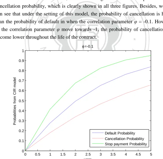
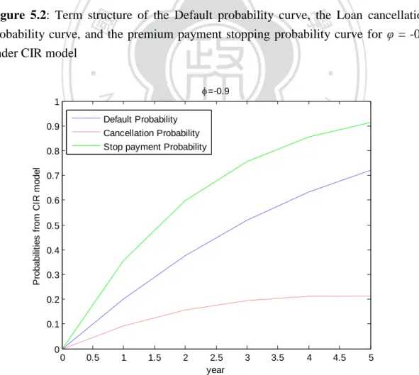
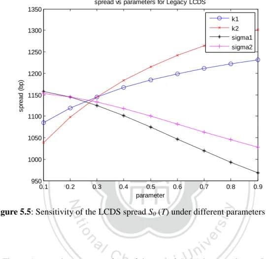
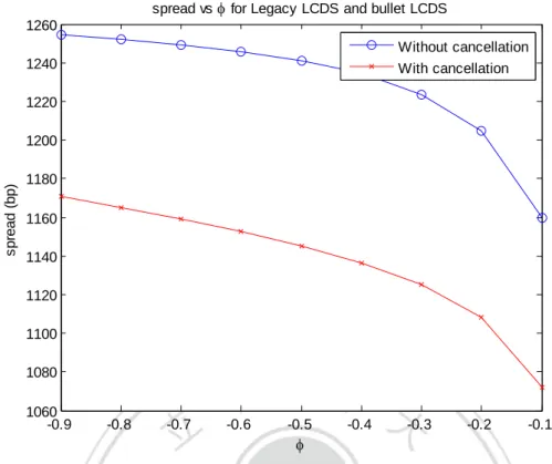
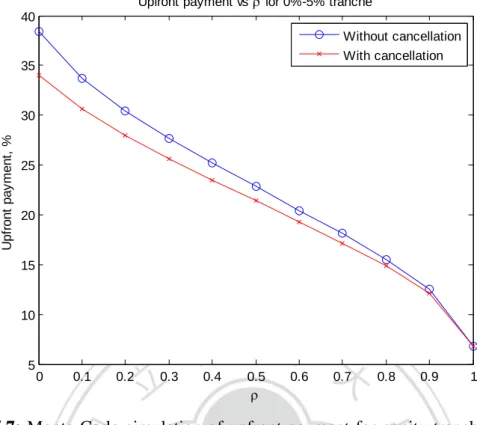
(5) Figures Figure 3.1: Loan CDS Mechanics ................................................................................. 8 Figure 3.3: The Tranched LCDX Structure................................................................. 12 Figure 5.1: Term structure of the Default probability curve, the Loan cancellation probability curve, and the premium payment stopping probability curve for υ = -0.1 under CIR model .......................................................................................................... 39 Figure 5.2: Term structure of the Default probability curve, the Loan cancellation probability curve, and the premium payment stopping probability curve for υ = -0.5 under CIR model .......................................................................................................... 40 Figure 5.3: Term structure of the Default probability curve, the Loan cancellation probability curve, and the premium payment stopping probability curve for υ = -0.9 under CIR model .......................................................................................................... 40 Figure 5.4: Term structure of the LCDS spread S0 (T) for (k1, θ1, σ1, k2, θ2, σ2) = (0.3, 0.3, 0.2, 0.3, 0.3, 0.2) and (𝑋𝑡, 𝑋𝑡1, 𝑋𝑡2) = (0.1, 0.2, 0.2) ........................................ 41 Figure 5.5: Sensitivity of the LCDS spread S0 (T) under different parameters........... 42 Figure 5.6: Spread S0 (T) with and without cancellation computed under parameters (k1, θ1, σ1, k2, θ2, σ2) = (0.3, 0.3, 0.2, 0.3, 0.3, 0.2) and (𝑋𝑡, 𝑋𝑡1, 𝑋𝑡2) = (0.1, 0.2, 0.2) ...................................................................................................................................... 43 Figure 5.7: Monte Carlo simulation of upfront payment for equity tranche with and without cancellation risk, assuming independence ...................................................... 44 Figure 5.8: Monte Carlo simulation of upfront payment for junior mezzanine tranche with and without cancellation risk, assuming independence ....................................... 44 Figure 5.9: Monte Carlo simulation of spread for senior mezzanine tranche with and without cancellation risk, assuming independence ...................................................... 45 Figure 5.10: Monte Carlo simulation of spread for junior senior tranche with and without cancellation risk, assuming independence ...................................................... 45 Figure 5.11: Monte Carlo simulation of spread for super senior tranche with and without cancellation risk, assuming independence ...................................................... 46 Figure 5.12: Monte Carlo extended single factor Gaussian copula simulation of upfront payment for equity tranche.............................................................................. 47 Figure 5.13: Monte Carlo extended single factor Gaussian copula simulation of upfront payment for junior mezzanine tranche ............................................................ 48 Figure 5.14: Monte Carlo extended single factor Gaussian copula simulation of spread for senior mezzanine tranche ............................................................................ 48 Figure 5.15: Monte Carlo extended single factor Gaussian copula simulation of spread for junior senior tranche ................................................................................... 49 Figure 5.16: Monte Carlo extended single factor Gaussian copula simulation of V.

(6) spread for super senior tranche .................................................................................... 49 Figure 5.17: Monte Carlo extended single factor Gaussian copula simulation of upfront payment for equity tranche.............................................................................. 51 Figure 5.18: Monte Carlo extended single factor Gaussian copula simulation of upfront payment for junior mezzanine tranche ............................................................ 51 Figure 5.19: Monte Carlo extended single factor Gaussian copula simulation of spread for senior mezzanine tranche ............................................................................ 52 Figure 5.20: Monte Carlo extended single factor Gaussian copula simulation of spread for junior senior tranche ................................................................................... 52 Figure 5.21: Monte Carlo extended single factor Gaussian copula simulation of spread for super senior tranche .................................................................................... 53. VI.

(7) Tables Table 3.2: Comparison of standard CDS and Loan CDS ............................................ 10 Table 5.1 Expected Loss for Legacy and Bullet LCDX tranche swap ....................... 54 Table 5.2 Expected Loss Percentage for Legacy and Bullet LCDX tranche swap ..... 55 Table 5.3 Leverage Ratio of Expected Loss for Legacy and Bullet LCDX tranche swap ............................................................................................................................. 56 Table 5.4 Unexpected Loss for Legacy and Bullet LCDX tranche swap ................... 58 Table 5.5 Unexpected Loss Percentage for Legacy and Bullet LCDX tranche swap . 58 Table 5.6 Leverage Ratio of Unexpected Loss for Legacy and Bullet LCDX tranche swap ............................................................................................................................. 59 Table 5.7 Greek Ratios — Tranche DELTA............................................................... 61 Table 5.8 Greek Ratios — Tranche GAMMA ............................................................ 62 Table 5.9 Result of Tranche Delta Hedging for Legacy LCDX tranche swap ........... 63 Table 5.10 Result of Tranche Delta Hedging for Bullet LCDX tranche swap ........... 64. VII.

(8) 1. Introduction. 1.1 Background For the past twenty years, the credit derivatives market has experienced meteoric growth with a variety of new products being introduced to the market. These new products was essential to the emergence of innovative hedging and investment strategies, but their leverage functions can also significantly increase existing risks, raising the difficulty for market participants and rating agencies to capture their risk characteristics and to price these products. In recent years, the complexity of the new products had caused worldwide financial crisis, not to mention the 2008 subprime crisis. Therefore, studies of the properties of credit derivatives are now attracting a great deal of interests for both market practitioners and academics. Fast growing new credit derivatives include standard credit default swaps (CDSs) of asset-backed securities and loan-only credit default swaps (LCDSs) of secured bank loans. These credit derivatives initially played roles in insurance, but later turn into credit instruments for investors or speculators, spreading the risk from large financial institutions to individuals. An LCDS is similar to a standard CDS, but with some differences. The main difference between a standard CDS and an LCDS is that the reference obligation for an LCDS is a syndicated secured bank loan, as opposed to a unsecured bond. On 8 June 2006, the International Swaps and Derivatives Association (ISDA) published an LCDS template for the US market, a watershed event expected to boost LCDS demand. Subsequently, the index product of the LCDS, Markit LCDX North American index was launched in May 2007. This increases transaction liquidity due to the convenience of standardized terms and execution. However, by the end of July 2007, concerns of the global housing bubble started to drag down asset prices and liquidity diminished. Besides, the early termination feature for LCDS also made the product challenging to value. According to statistics from DTCC, the gross notional for Markit LCDX has decreased from 250,000 million to 150,000 between October 2008 and February 2010. As a result, a new bullet version of the U.S. LCDS product, so called Bullet LCDS was launched on April 5, 2010 by publishing revised transaction documentation and announcing market practice changes to the LCDS market. The key change of new Bullet LCDS was the migration to a ―bullet maturity‖ product through the removal of the early termination feature. By doing so, the International Swaps and Derivatives Association (ISDA) harmonized the contracts and conventions of the LCDS with the standard CDS for the purpose to enhance liquidity of LCDS market. 1.

(9) Despite the change of the LCDS contracts, still a great proportion is traded on the LCDS with early termination, known as the Legacy LCDS. In fact, market practitioners today still use the CDS pricing model to price loan CDSs without considering the cancellation nature of the loans, which causes inaccuracy in the spread prices for loan credit derivatives. Therefore, pricing difficulties of the early termination remain unsolved, and still awaits for further study on the cancellation topic. In pricing loan credit derivatives, the main idea is to determine the default probability and the cancellation probability. The two primary types of credit risk models are the structural-form models and reduced-form (or intensity-based) models. Structural-form models are based on the Merton model, in which company equity can be regarded as European call options. Reduced-form models are not determined by the value of the firm, but by the first jump of an exogenous jump process. The parameters (intensities) governing the default hazard rate or the loan cancellation rate can be inferred from market data. Under the reduced-form framework, we can incorporate correlations between default time and cancellation time by allowing stochastic process of the intensities are correlated. In this paper, we develop the pricing formulas for Legacy LCDS (with cancellation feature) and also extend to its index product the LCDX tranche swap, which is introduced in the latter part of this paper. Then, an sensitivity analysis is presented to point out the importance of the role for the correlation between default and cancellation. Furthermore, a comparison of pricing and hedging between Legacy LCDS and Bullet LCDS as well as Legacy LCDX tranche swap and Bullet LCDX tranche swap is demonstrated. The pricing of the new Bullet LCDS and LCDX tranche swap can be done by simply taking out the cancellation features from the models.. 2.

(10) 1.2 Research targets From the paragraph above, we state that market today has developed the bullet LCDS to remove the cancellation feature from syndicated loan derivatives considering the liquidity of the products; however, still a great proportion is traded on the Legacy LCDS with early termination. Besides, market practitioners today still use the CDS pricing model to price loan CDSs without considering the cancellation nature of the loans, which causes inaccuracy in the spread prices for loan credit derivatives. In this paper, we introduce two different models to handle the cancellation feature, which is presented in the LCDS and LCDX tranche contracts. First, for the LCDS, we followed a industry standard model and introduced the general intensity-based model. Closed-form solutions for this model can be obtained under Affine Jump Diffusion specifications through a set of Riccati equations. In this thesis, explicit formulas are derived under the CIR parameterization. Second, for the LCDX tranche swap, we introduce the one factor Gaussian copula framework which closely follow the Merton structural framework, where dynamic of both default and cancellation are determined by the underlying firm value model. Here, we extend the single factor Gaussian copula model with a new variable to include the cancellation risk for loan products. As the first target of this thesis, we try to focus on the role of correlations ρ and υ, where correlation parameter ρ stands for the correlation between the underlying asset value and the macro factor M, while the correlation parameter υ stands for the correlation between default and cancellation. Thus, we conduct a sensitivity analysis for LCDS and the LCDX tranche swap in order to find out what happens when the two correlations comes to work. For the second target of the thesis, we look into the risk characteristics of the loan credit derivatives. Apart from examining the risk characteristics for the LCDS and LCDX tranche swap alone, we are also interested in the change in risk characteristics between Legacy LCDS and Bullet LCDS (with and without cancellation). Therefore, in our result we show a comparison of the cancellable and non-cancellable LCDSs including the risk measurements for expected loss and unexpected loss. Last, following the previous target, we go even further to consider the hedging issue for loan credit derivatives to give concluding remarks for market practitioners. We compute the Greeks and hedge positions for the LCDX tranche swap, and again compare the numerical results with the Bullet version (without cancellation) of the products.. 3.

(11) 1.3 Organization The rest of the thesis is organized as follows. In Chapter 2, we review previous works on the pricing and hedging issues of the LCDS and LCDX. Chapter 3 describes the structure of a LCDS product and its valuation techniques as well as the LCDX tranche swap. Following the introduction of the products, we elaborate on the settings of the intensity-based model proposed by Wei (2007). Next, we move on to a extended one factor Gaussian copula model for pricing LCDX tranche swap. Furthermore, in Chapter 4 we introduce the credit risk measurements and hedging technique for the loan credit derivatives. The pricing and hedging results on LCDS and LCDX tranche swap are presented in Chapter 5. We show the results from our sensitivity analysis in terms of different correlations ρ and υ. Moreover, we examine the risk characteristics and hedging costs for LCDS and LCDX tranche swap compared to their bullet version. Finally, we conclude our findings and observations in the last chapter.. 4.

(12) 2. Literature Review. Loan credit default swaps (LCDSs) is a agreement between two parties to exchange credit risk at the occurrence of a credit event, which acts as a insurance to the protection buyer. LCDSs are very similar to standard credit default swaps (CDSs), except that other than default risk, the LCDS contract is also exposed to cancellation risk due to the possibility of prepayment of loans before maturity. Hence, the LCDS contract is cancellable and have higher recovery rates. Even though LCDS and CDS operate on two separate markets, since they have the same underlying reference entity, Morgan and Zheng (2007) supposed that the both LCDS and CDS must also share the same probabilities of default (or default intensities). Consequently, the relationship for the two instruments can be expressed as 𝑠𝑝𝑟𝑒𝑎𝑑𝐿𝐶𝐷𝑆 𝑠𝑝𝑟𝑒𝑎𝑑𝐶𝐷𝑆 = 1 − 𝑅𝑒𝑐𝑜𝑣𝑒𝑟𝑦𝐿𝐶𝐷𝑆 1 − 𝑅𝑒𝑐𝑜𝑣𝑒𝑟𝑦𝐶𝐷𝑆. (2.1). Equation 2.1 gives a rough approximation between the two different instruments. However, from market spreads, it is shown that the equation above clearly does not hold, which the LCDS spreads are sometimes much higher than the recovery-adjusted CDS spreads. In order to solve this puzzle, Peter Dobranszky (2008) tried to find stochastic risk factors that may provide the link between CDS and LCDS markets and explain the current market figures and their dynamics by incorporating the possibility of negative correlation between default and cancellation intensities and the possibility of stochastic recovery rate correlated with the default intensity. The inequality of the above equation possibly stream from different conventions in the contracts between CDSs and LCDSs, resulting in more difficult modeling issues for LCDSs, simply not only higher recovery rates. From an LCDS modeling perspective, here we summarize several key factors that need to be considered: (1) (2) (3) (4). default risk cancellation risk higher recovery rate correlation between cancellation and probability of default. The correlation aspect is the most difficult part, while, intuitively, a negative correlation between cancellation and the probability of default can be observed from 5.

(13) empirical results. For the pricing of LCDSs, prevailing approaches follow the industry standard approach with deterministic intensity that JP Morgan (2001) originally introduced in the valuation of standard CDSs. In 2007, Scott et al (2007b), from JP Morgan, considered a simple mark-to-market approach using a historical cancellation probability matrix. Also, Elizalde et al (2007) from Merrill Lynch introduced a generic LCDS modeling framework that incorporated a refinancing rate into the modeling of the cancellation feature. The same year, Morgan and Zheng (2007) of Lehman Brothers designed a generalized model based on the hazard rate model in pricing standard CDSs while assuming independence between cancellation and default. Later, Wei (2007) pointed out the limitations of the prior approaches and extended this framework further by incorporating stochastic intensity, which he borrowed the short rate model for the pricing of bonds to derive a closed-form partial differential equation solution under CIR specification. Under the stochastic intensity framework, Wang and Liang (2012) consider the pricing of both a single-name and a two-reference basket LCDS and Wang, Liang and Yang (2012) extended this framework into N baskets as well. From a different aspect, Wu and Liang (2012) extended the model into a multifactor case by incorporating stochastic recovery. Other non-standard approaches are developed by Bandreddi et al (2007) from Merrill Lynch who used a double-barrier model with Gaussian distribution instead of Poisson distribution so that the cancellation barrier and the default barrier behave as two competing factors. A survey of the LCDS pricing models can be found in Ong, Li and Lu (2012). Furthermore, for the pricing of the index product of the credit derivatives, the industry has accepted the copula method to model joint default behavior of names in the basket, which was introduced by Li (2000). One of the key assumptions of the one factor Gaussian copula model is that the asset values of the names in the underlying reference portfolio are correlated to a common macroeconomic factor with the same correlation for all single names. Using the one factor Gaussian copula framework, Shek et al (2007) extend the model with a new variable to incorporate the cancellation feature for the index loan derivatives, including the LCDX index swap and LCDX tranche swap. While, Dobranszky and Schoutens (2008) extended the approach to the generic one-factor Levy copula. However, in the double barrier one-factor copula approach, the default barrier needs to be lower than the prepayment barrier. This requirement could be violated when the default probability and the cancellation probability are high. Michael Liang (2009), from industrial bank in China provide a simple two-factor Gaussian copula model to price the LCDX tranche swap with cancellation risk. 6.

(14) In this article we do not intend to develop a new model for LCDSs, rather we assume that a model for LCDSs is already in use. For the valuation of LCDSs, we consider a industry standard intensity model incorporated with stochastic intensity which was first introduced by Wei (2007). Similarly, to model a tranched portfolio of LCDSs, the LCDX tranche swap, here we refer to Shek et al (2007), who introduced a extended double barrier single factor Gaussian copula model to deal with the cancellation issue. For the risk measurement of the more complicated LCDX tranche swap, we follow Gibson (2004) who introduced the expected and unexpected risk measures to examine tranche risk of the synthetic CDOs. Moreover, Chiang, M., Yueh, M., and Lin, A. (2009) proposed a Delta hedge analysis to determine hedging costs for synthetic CDO tranches under a hypothesis portfolio. In this thesis, we conduct a hedging analysis based on the methods referring to their works.. 7.

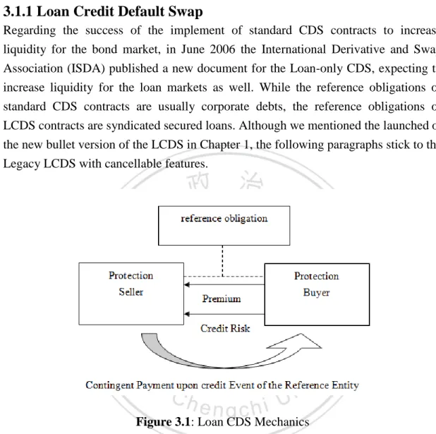
(15) 3 3.1. Valuation Framework Product Outline. 3.1.1 Loan Credit Default Swap Regarding the success of the implement of standard CDS contracts to increase liquidity for the bond market, in June 2006 the International Derivative and Swap Association (ISDA) published a new document for the Loan-only CDS, expecting to increase liquidity for the loan markets as well. While the reference obligations of standard CDS contracts are usually corporate debts, the reference obligations of LCDS contracts are syndicated secured loans. Although we mentioned the launched of the new bullet version of the LCDS in Chapter 1, the following paragraphs stick to the Legacy LCDS with cancellable features.. Figure 3.1: Loan CDS Mechanics Except for the difference of reference obligations of the contracts, standard CDS and Loan CDS simply share the same mechanics. Figure 3.1 gives a simply image of how this mechanism works. An LCDS is an over-the-counter credit derivative, which responds to two classes of events that result in early termination of the contract, credit and cancellation events. On one hand, the protection buyer pays a periodical fixed spread to the protection seller throughout the life of the contract. On the other hand, the protection seller pays an amount to cover the losses of the protection buyer upon default. If a credit event occurs prior to the maturity of the contract, the contract is terminated and no further premium payments are due, whereas the accruals premium upon the termination date should still be given to the protection seller. Similar to a credit event, when a cancellation event occurs (loans are prepaid), the contract is 8.

(16) terminated and no further premium payments are due. However, this time the protection seller makes no payments to the protection buyer. The emergence of the LCDS contract has a huge impact on loan investors. Before the inception of the LCDS contracts, investors can only long risk on loans, with little or no ability for participants to go short risk or take on risk synthetically. Now, the rule of the loan markets have been changed, allowing investor to trade and take on risks similar to the standard CDS contract. According to the JPMorgan Credit Derivatives Handbook, benefits of the LCDS contracts include the followings:  The ability to implement a bullish view (sell LCDS protection) without having to access the primary or secondary market for cash loans. The ability to create   . levered portfolios of secured risk. The ability to hedge or implement bearish views on loans (buy LCDS protection) and be short risk in what has traditionally been a long-only market. The ability to trade cross-asset views such as a view on the senior debt spread versus loan spread. The ability to implement curve shape positions and views once the market develops and a LCDS spread curve becomes available.. LCDS contracts are based on the standard CDS contract; however, with several modifications to address the unique nature of the loan market. We discuss some major differences in the following section.. 3.1.2 Comparison of Standard CDS and Loan CDS Having discussed the general structure of an LCDS, we now summarize the key differences between an LCDS and a standard CDS as a starting point for LCDS pricing. The first difference is that the deliverable debt security in a LCDS contract is a syndicated senior secured loan. In contrast, the deliverable securities in a standard CDS contracts are, loans or, more commonly, bonds with different seniority and security characteristics. Therefore, under the LCDS contract, a credit event is recognized only when the reference entity (1) files for bankruptcy (or its equivalent) or (2) fails to pay the principal or interest. Different from standard CDSs, LCDSs do not typically include restructuring as a credit event that triggers settlement of the contract. Besides, standard CDS contracts are generally not cancellable and remain active through their scheduled maturity if no credit events occur. On the other hand, 9.

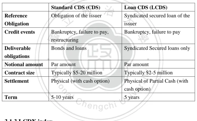
(17) since the deliverable securities in a LCDS contract are loans, LCDS contracts can be canceled (also called calling, prepayment) if no loan of designated priority is outstanding. Intuitively, for a given reference name, standard CDS and LCDS spreads should imply the same default probability, but different recovery rates. Research has revealed that syndicated bank loan recoveries are considerably higher than unsecured bonds both on average and over the credit cycle. The widely accepted recovery rates for secured bank loans are 70% while, for senior unsecured bonds, the recovery is 40%. Here, we show the other differences of the contracts in the following Table 3.2. Table 3.2: Comparison of standard CDS and Loan CDS Standard CDS (CDS). Loan CDS (LCDS). Reference Obligation. Obligation of the issuer. Syndicated secured loan of the issuer. Credit events. Bankruptcy, failure to pay, restructuring. Bankruptcy, failure to pay. Deliverable obligations. Bonds and loans. Syndicated Secured loans only. Notional amount. Par amount. Par amount. Contract size. Typically $5-20 million. Typically $2-5 million. Settlement. Physical (with cash option). Physical of Partial Cash (with cash option). Term. 5-10 years. 5 years. 3.1.3 LCDX index Now we have introduce the mechanics of LCDS and its comparison to the standard CDS, in this section, we go further to introduce its index product, the LCDX index and Tranched LCDX. LCDX is a tradable index which consists 100 equally-weighted underlying single-name LCDSs. The 100 LCDS contracts each reference an entity whose loans trade in the secondary loan market, and in the more recent LCDS market. The index is being brought to market by CDS Index Co, a firm backed by a consortium of dealer banks active in the credit derivatives market. These indices are administered by Markit, which also acts as the licensing, marketing and calculation agent for the indices. ISDA and Cleary have also been active participants in the drafting of the 10.

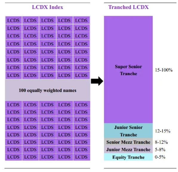
(18) trade documentation and auction rules. In terms of trading, the LCDX is traded on price terms with fixed spread and maturity set to 5 Years. Upfront payments are simply par minus price. The index will trade on a factor if a credit is removed and roll dates are April 3rd and October 3rd. Unlike the index product for standard CDS, so called the CDX, which is only affected by credit events, LCDX has two classes of events by which a credit is removed from the index, including a credit event and the cancellation of loans. LCDX index- Credit event There are two events that would trigger a payment from the buyer (protection seller) of the index, which are (1) bankruptcy or (2) failure to pay a scheduled payment on any debt for any of the reference names of the index. Once the credit event is announced, ISDA will congregate the major participants in the market and agree an event determination date. Coupons will stop accruing on the defaulted entity on this date. An auction will most likely be announced for a date approximately 3 weeks after the credit event to set the recovery price for the deliverable loans. Then, a new version of the index will be issued with the defaulted entity removed and with a reduced notional. Until the credit event is settled, both versions of the index may trade – one with and one without the defaulted entity. LCDX index- Cancellation of LCDSs Unlike standard CDS, the LCDS contract is cancellable if an issuer repays its debt without issuing new senior syndicated secured debt. This has been a regular occurrence in the loan market, especially when an issuers rating moves from high-yield to investment grade during economic upturns. When a credit has repaid its debt, the name is polled for and removed from the syndicated secured list. This triggers an automatic 30 business day search period in which new debt is searched for (this allows time for companies who re-finance their debt to get their new debt into the market) and if after 30 days no new debt is found the name is removed from the index with a dealer vote.. 3.1.4 Tranched LCDX The Tranched LCDX is constructed from the LCDX index using a typical CDO capital structure. A tranche provides access to customized risk by allocating the payouts on a pool of assets to a collection of investors. Each investor will be exposed to losses at different levels of subordination and will therefore receive different levels 11.

(19) of compensation for this risk. Just as a LCDS contract provides exposure to the credit risk of a reference company, and the LCDX index provides exposure to the risk of a portfolio of credits, a tranche LCDX provides exposure to the risk of a particular amount of loss on a portfolio of companies. As such, a tranche references a portfolio of companies and defines the amount of portfolio loss against which to sell or buy protection.. Figure 3.3: The Tranched LCDX Structure The tranche instrument is a result of the capital structure framework, which translates a set of assets (the reference portfolio) into a set of liabilities (the tranche risk). Figure 3.3 shows an illustration of how this capital structure works. Equity tranches, which are attached at 0%, are exposed to the first losses on the portfolio. Mezzanine tranches, which have more subordination, are not exposed to portfolio losses until the portfolio losses exceed the lower attachment point of the tranche. Senior tranches have the most subordination and thus the least exposure to portfolio losses. The tranches traded on LCDX are 0-5% (equity), 5-8% (junior mezzanine), 8-12% (senior mezzanine), 12.

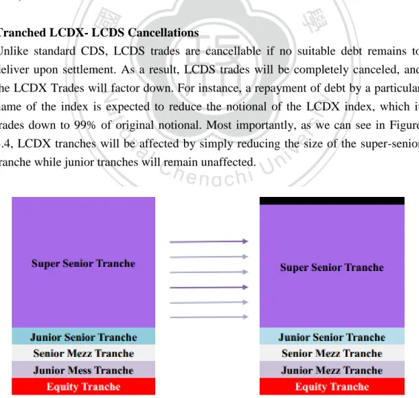
(20) 12-15% (junior senior), and 15-100% (super senior). In terms of trading, the equity tranche and the senior mezzanine tranche are quoted in upfront payments ( no running spread) while the more senior tranches are quoted in running spread similar to the LCDS contract. Tranched LCDX- Credit Events Credit Events for Tranche LCDX are defined as for LCDX, including failure to pay, and bankruptcy. The credit event settlement will use LCDS Auction Settlement Price. When the first default occurs, it reduces the notional of the equity tranche. The reduction continues as more default occurs until the equity tranche is all wiped out, and then it moves on to the more senior tranches. Thus, new tranche size and new attachment/detachment points depends on total cumulative losses to date. For example, after 2% of losses in whole portfolio from 3 defaults, the new attachment/detachment points are equal to the (original attachment point – losses to date) / index factor. Then, we compute index factor after 3 defaults = 0.97, and 5% Attachment Point now = (5% - 2%) / 0.97 = 3.09%. Tranched LCDX- LCDS Cancellations Unlike standard CDS, LCDS trades are cancellable if no suitable debt remains to deliver upon settlement. As a result, LCDS trades will be completely canceled, and the LCDX Trades will factor down. For instance, a repayment of debt by a particular name of the index is expected to reduce the notional of the LCDX index, which it trades down to 99% of original notional. Most importantly, as we can see in Figure 3.4, LCDX tranches will be affected by simply reducing the size of the super-senior tranche while junior tranches will remain unaffected.. Figure 3.4: The LCDS cancellation for Tranched LCDX 13.

(21) 3.2 Modeling Loan CDS The intensity-based model, also called the reduced-form model, defines the dynamics of a stopping time (either default or cancellation) by a exogenously given intensity process under the risk-neutral probability measure Q. The intensity-based model was first developed independently by Jarrow and Turnbull (1995) and Madan and Unal (1998). Many follow-up papers can be found in Jarrow and Yu (2001), Lando (2004) and references therein. In this paper, we refer to Wei (2007), who first incorporated stochastic intensity into the intensity-based model for the pricing of LCDS. The reason to define a stochastic intensity rather than a constant intensity is that when the constant intensity for cancellation (λ2) is considered, the cancellation effect do not play a significant role in determining for the LCDS spread under the intensity-based model. Thus, by making the intensities stochastic, we can analyze the changes of the spread when we take the cancellation feature into account. In order to incorporate the stochastic intensities, we borrow the concept of a short rate model. By using the Feynman-Kac approach and solving the Riccati equations with the boundary conditions, we can arrive at a close-form solution for the default and survival probabilities and further compute the spread for LCDS. Before we start the valuation of LCDSs, first we have to state the following notations.  T1 = the default time of the reference entity  T2 = the calling time of the secured loan  T = the maturity of LCDS contract  R = recovery rate  r = risk free rate  ti = coupon payments dates for i=1,...,m.  ∆i = day count fraction for payment period i . St = fair LCDS spread at time t. The main idea of the intensity models is to be able to explicitly determine the default and cancellation probability through intensities. Suppose the two driving intensities for default and cancellation are namely λ1 and λ2, the default and cancellation probability at time t can be express as the following: 𝑄𝑡 𝑇 𝑖 < 𝑠 = 1 − 𝐸[𝑒 −. 𝑠 𝑖 𝑡 𝜆 𝑢 𝑑𝑢. ]. (3.1) 14.

(22) Similarly, the survival probability of the individual events at time t are 𝑄𝑡 𝑇 𝑖 > 𝑠 = 𝐸[𝑒 −. 𝑠 𝑖 𝜆 𝑑𝑢 𝑡 𝑢. ]. (3.2). where i=1,2 Also, the survival probability of both event at time t is 𝑄𝑡 𝜏 > 𝑠 = 𝑄𝑡 𝑇1 > 𝑠, 𝑇 2 > 𝑠 = 𝐸𝑡 [𝑒 −. 𝑠 𝑡. 𝜆 1𝑢 +𝜆 2𝑢 𝑑𝑢. ]. (3.3). where 𝜏 = 𝑇 1 ∧ 𝑇 2 is the first occurrence of two stopping time Similar to the standard CDS, the LCDS contract usually specifies two potential cash flows. The default leg determines the present value of the cash flows that the protection buyer expects to receive; on the other hand, the fixed premium leg determines the present value of the cash flows that the protection buyer expects to pay. The value of the LCDS contract to the protection buyer is the difference between the present value of the default leg (DL) and that of the premium leg (PL): 𝑉𝑎𝑙𝑢𝑒 𝑜𝑓 𝐿𝐶𝐷𝑆 = 𝑃𝐿 − 𝐷𝐿. (3.4). Suppose that the maturity of the contract is T, the spread for the contract at time t is St and the face value is 1. We assume premium are paid on t1<t2<···<tm=T, and that ∆i stands for the time interval between two payment dates, which is three months according to the LCDS contract. From the protection seller perspective, when the reference entity confronts a stopping time (either default or cancel), there is no more cash flow generated except for the accrued premium payment since the last payment date. Thus the premium leg of the LCDS contract can be express as a stream of payments StCm at payment dates tm until min(T1, T2, T) plus any remaining accruals. The expected present value of the premium stream is given by 𝑆𝑡 𝐸𝑡. 𝑡 𝑖 ≥𝑡. 𝑒 −𝑟(𝑡𝑖 −𝑡) ∆𝑖 1 𝜏>𝑡𝑖. = 𝑆𝑡. 𝑡 𝑖 ≥𝑡. 𝑒 −𝑟. 𝑡 𝑖 −𝑡. ∆𝑖 𝑄𝑡 (𝜏 > 𝑡𝑖 ). (3.5). The expected present value of the premium accrual since default or loan cancellation is. 15.

(23) 𝑒 −𝑟(𝜏−𝑡). 𝑆𝑡 𝐸𝑡 𝑡 𝑖 ≥𝑡. ∆𝑖 𝑡𝑖 − 𝑡𝑖−1. = 𝑆𝑡 𝑡 𝑖 ≥𝑡. = −𝑆𝑡 𝑡 𝑖 ≥𝑡. 𝜏 − 𝑡𝑖−1 ∆1 𝑡𝑖 − 𝑡𝑖−1 𝑖 𝑡∨𝑡𝑖−1 <𝜏≤𝑡𝑖. 𝑡𝑖. 𝑒 −𝑟. 𝑠−𝑡. 𝑠 − 𝑡𝑖−1 𝑑𝑄𝑡 (𝜏 ≤ 𝑠). 𝑡∨𝑡 𝑖−1 𝑡𝑖. ∆𝑖 𝑡𝑖 − 𝑡𝑖−1. 𝑒 −𝑟. 𝑠−𝑡. 𝑠 − 𝑡𝑖−1. 𝑡∨𝑡 𝑖−1. 𝑑𝑄𝑡 (𝜏 > 𝑠) 𝑑𝑠 𝑑𝑠. (3.6). Hence, here we sum up Equation (3.5) and Equation (3.6) and multiple the combination of the two with the LCDS spread, then we can obtain the present value of the premium leg at time t for the LCDS contract.. ∆𝑖 𝑒 −𝑟. 𝑃𝐿𝑡 = 𝑆𝑡. 𝑡 𝑖 −𝑡. 𝑄𝑡 𝜏 > 𝑡𝑖. 𝑡 𝑖 ≥𝑡 𝑡𝑖. 1 − 𝑡𝑖 − 𝑡𝑖−1. 𝑒 −𝑟. 𝑠−𝑡. 𝑠 − 𝑡𝑖−1. 𝑡∨𝑡 𝑖−1. 𝑑𝑄𝑡 (𝜏 > 𝑠) 𝑑𝑠 𝑑𝑠. (3.7). On the other hand, the default leg is subject to loss only when T1 < min(T2, T), which means that default occurs prior to cancellation and the maturity of the contract. Also, since there is a chance of recovery for loan defaults, we deduct the amount of recovery from the losses. Here, we assume the recovery rate R is independent of T1, T2 and has expected value 𝑅 . Thus, the present value of the default leg can be expressed as 𝐷𝐿𝑡 = 𝐸𝑡 𝑒 −𝑟. 𝑇 1 −𝑡. 1 − 𝑅 1 𝑇 1 <𝑚𝑖𝑛 (𝑇 2 ,𝑇). ∞. 𝜈∧𝑇. = (1 − 𝑅 ). 𝑒 𝑡. 𝑡. −𝑟(𝑢−𝑡). 𝑑 2 𝑄𝑡 (𝑇 1 > 𝑢, 𝑇 2 > 𝜐) 𝑑𝑢𝑑𝜈 𝑑𝑢𝑑𝜈. 𝑇. 𝑒 −𝑟. = 1−𝑅. 𝑢−𝑡. 𝐸𝑡 𝜆1𝑢 𝑒 −. 𝑢 𝑡. 𝜆 1𝑠 +𝜆 2𝑠 𝑑𝑠. 𝑑𝑢. (3.8). 𝑡. where it follows that 𝑢, 𝑣 ≥ 𝑡. Equation (3.8) infers that the value of the default leg is the expected discount value of the loss at default, where the discount factor is the risk free discounting factor 𝑒 −𝑟. 𝑢 −𝑡. times the conditional probability of no loan 16.

(24) cancellation 𝑄𝑡 𝑇 2 > 𝑢 = 𝐸𝑡 [𝑒 −. 𝑢 𝑡. 𝜆 2𝑠 𝑑𝑠. ]. Hence, by equating the premium leg and the default leg, we can compute the value of the LCDS spread at time t as. 𝑆𝑡 =. 𝑢 1 2 𝑇 −𝑟(𝑢−𝑡) 𝑒 𝐸𝑡 [𝜆1𝑢 𝑒 − 𝑡 𝜆 𝑠 +𝜆 𝑠 𝑑𝑠 ]𝑑𝑢 𝑡 𝑒 −𝑟 𝑡𝑖 −𝑡 𝑄𝑡 𝜏 > 𝑡𝑖 𝑡𝑖 𝑑𝑄𝑡 (𝜏 > 1 𝑡 𝑖 ≥𝑡 ∆𝑖 −𝑡 − 𝑡 𝑒 −𝑟 𝑠−𝑡 𝑠 − 𝑡𝑖−1 𝑡∨𝑡 𝑑𝑠 𝑖−1 𝑖 𝑖−1. (1 − 𝑅 ). (3.9) 𝑠). 𝑑𝑠. So, from the above equation, we see that the LCDS spread St is completely determined by 𝑄𝑡 𝜏 > 𝑠 ,. 𝑑𝑄𝑡 (𝜏>𝑠) 𝑑𝑠. , 𝐸𝑡 [𝜆1𝑢 𝑒 −. 𝑢 𝑡. 𝜆 1𝑠 +𝜆 2𝑠 𝑑𝑠. ] . Since we assume. stochastic intensities for default and cancellation, thus through the specification of the CIR process, we can derive a closed-form partial differential equation solution and simply solve the three mathematical forms above. A detailed operation and technical computations of the model is demonstrated in the following sections.. 3.2.1 Intensity-based model In this section, we introduce the concept of the intensity (default intensity is also called the hazard rate), and how we deal with the stochastic intensity in this model. First, given a probability space (𝛺, ℱ, ℱ. 𝑡≥0 , 𝑃),. let τ be the ℱ ‒ stopping. time at which default occurs, with a distribution function 𝐹 𝑡 = 𝑃 𝜏 ≤ 𝑡 and the probability density function f(t). We define the hazard function as the probability that default will occur in the interval (𝑡, 𝑡 + ∆𝑡), given that the reference entity has survived up to time t. Definition 3.1 The distribution function F(t) for intensity is defined as 𝐹 𝑡 = 1 − 𝑒−. 𝑡 0𝜆. 𝑢 𝑑𝑢. where 0 ≤ 𝑡 < 𝑇. proof. 𝜆 𝑡 = 𝑙𝑖𝑚 𝑃 𝑡 < 𝜏 ≤ 𝑡 + ∆𝑡 𝜏 > 𝑡 △𝑡⟶0. 17.

(25) 𝑃 𝑡 < 𝜏 ≤ 𝑡 + ∆𝑡 𝜏 > 𝑡 △𝑡⟶0 𝑃(𝜏 > 𝑡). = 𝑙𝑖𝑚. =. 𝑡+∆𝑡 𝑓 𝑢 𝑑𝑢 𝑡 𝑙𝑖𝑚 ∞ △𝑡⟶0 𝑓 𝑢 𝑑𝑢 𝑡. =. 𝑓(𝑡) 1−𝐹 𝑡. 𝜕 𝐹(𝑡) = 𝜕𝑡 1−𝐹 𝑡 =−. 𝜕 𝑙𝑜𝑔(1 − 𝐹 𝑡 ) 𝜕𝑡. Then, solving the differential equations, we get 𝐹 𝑡 = 1 − 𝑒−. 𝑡 0𝜆. 𝑢 𝑑𝑢. (3.10). 𝑓(𝑡) = 𝜆 𝑡 𝑒 −. 𝑡 0𝜆. 𝑢 𝑑𝑢. (3.11). and. Also, if we define the survival probability 𝑆 𝑡 = 1 − 𝐹 𝑡 = 𝑃(𝜏 > 𝑡), then 𝑆 𝑡 = 𝑒−. 𝑡 0𝜆. 𝑢 𝑑𝑢. (3.12). Now, we have defined the distribution function for the intensity, but in order to compute the spread for LCDS, we need to model the default time τ (or the stopping time of a credit event). The default time τ is usually modeled as a Cox process which is a generalization of the Poisson process where the intensity is allowed to be random, such that if conditioned on a particular realization of the intensity (allowing the intensity to be stochastic), the jump process becomes an inhomogeneous Poisson process. Under such a process, the default time τ is the first jump-time of a time-inhomogeneous counting process N(t). Thus, the default time τ is doubly stochastic. Definition 3.2 The counting process is defined by 𝑁 𝑡 =. 1 𝜏 ≤ 𝑡 𝑓𝑜𝑟 𝑡 > 0 0 𝑓𝑜𝑟 𝑡 = 0 18.

(26) where 1 𝜏 ≤ 𝑡 is the indicator function of the ℱ ‒ stopping time τ. Furthermore, the process satisfies the following conditions: 1. The increment 𝑁(𝑇) − 𝑁(𝑡) is independent of the σ - algebra ℱ𝑡 . 2. The increment 𝑁(𝑇) − 𝑁(𝑡) is distributed according to a Poisson law with a strictly increasing, non-negative, and invertible parameter 𝛬 𝑡 =. 𝑡 𝜆 0. 𝑢 𝑑𝑢. Definition 3.3 Let 𝜆(𝑡) be a nonnegative predictable process such that, for all t, we have. 𝛬 𝑡 =. 𝑡 0. 𝜆 𝑢 𝑑𝑢 < ∞ almost surely. Then a non-explosive adapted counting. process N(t) has 𝜆(𝑡) as its intensity if 𝑁 𝑡 − 𝛬 𝑡 is a local martingale. Now, we could write the intensity process as a function of the current level of state variables. These state variables include time, stock price, credit rating, and other relevant variables for predicting the likelihood of default. In this case, we would denote the intensity as 𝜆(𝑡) = 𝛬 𝑋(𝑡) , where X(t) is a stochastic process. Definition 3.4 If the intensity process λ of N(t) is ℱ𝑡 .-predictable, then N(t) is doubly stochastic if condition on the σ-algebra ℊ𝑡 ∨ ℱ𝑠 = 𝜍(ℊ𝑡 ⋃ℱ𝑠 ), 𝑁(𝑠) − 𝑁(𝑡) has a Poisson distribution with parameter. 𝑠 𝜆 𝑡. 𝑢 𝑑𝑢, 𝑤𝑕𝑒𝑟𝑒 ℱ𝑡 ⊂ ℊ𝑡 .. Under the doubly stochastic setting, it is easy to show that 𝑃 𝜏 > 𝑠 ℊ𝑡 = 𝑃(𝑁 𝑠 − 𝑁 𝑡 = 0 |ℊ𝑡 ) = 𝐸 𝑃(𝑁 𝑠 − 𝑁 𝑡 = 0 |ℊ𝑡 ∨ ℱ𝑠 ) |ℊ𝑡 = 𝐸 𝑒−. 𝑠 𝑡 𝜆. 𝑢 𝑑𝑢. |ℊ𝑡. (3.13). This equation is convenient for calculations, because evaluating the expectation in (3.13) is computationally equivalent to the standard financial calculation of default-free zero-coupon bond price, treating λ as a short-term. interest-rate process. Indeed, this analogy is also quite helpful for intuition when extending (3.13) to pricing applications. It is sufficient for the convenient survival-time formula (3.13) that 𝜆𝑡 = 𝛬 𝑋𝑡 for some measurable function 𝛬 𝑡 : ℝ𝑑 ⟶ [0, +∞), where X in ℝ𝑑 solves a stochastic differential equation of the form 𝑑𝑋𝑡 = 𝜇 𝑋𝑡 𝑑𝑡 + 𝜍 𝑋𝑡 𝑑𝐵𝑡. (3.14) 19.

(27) for some (ℊ𝑡 )-standard Brownian motion B in ℝ𝑑 . Here, 𝜇 𝑋𝑡 and 𝜍 𝑋𝑡 are functions on the state space of X that satisfy enough regularity for (3.14) to have a unique (strong) solution. With this, the survival probability calculation (3.15) is of the form 𝑃 𝜏 > 𝑠 ℊ𝑡 = 𝐸 𝑒 −. 𝑠 𝑡 𝛬. 𝑋(𝑢) 𝑑𝑢. |ℊ𝑡 = 𝑓(𝑋𝑡 , 𝑡). (3.15). where, under the usual regularity for the Feynman-Kac approach, f( · ) solves the partial differential equation (PDE) 𝛢𝑓 𝑥, 𝑡 − 𝑓𝑡 𝑥, 𝑡 − 𝛬 𝑥 𝑓(𝑥, 𝑡) = 0. (3.16). for the generator A of X, given by 𝛢𝑓 𝑥, 𝑡 =. 𝜕 𝑖 𝜕𝑥 𝑖. 1. 𝑓 𝑥, 𝑡 𝑢𝑖 𝑥 + 2. 𝜕2 𝑖,𝑗 𝜕𝑥 𝜕𝑥 𝑖 𝑗. 𝑓 𝑥, 𝑡 𝛾𝑖,𝑗 (𝑥). (3.17). where 𝛾(𝑥) = 𝜍(𝑥)𝜍(𝑥)𝑇 , with the boundary condition 𝑓 𝑥, 𝑠 = 1.. 3.2.2 Affine model for LCDS In this section, we give a brief review of the affine processes. Definitions for affine process can be found in Duffie, Filipovic and Schachermayer (2003). Dai, Le and Singleton (2006) extends the definition to construct a more general class of discrete-time dynamic models. In many financial applications that are based on a state process, such as the solution X of the SDE, a useful assumption is that the state process X is ―affine‖. Definition 3.5 We say that a N dimensional Markov process X is affine under measure Q if the conditional Laplace transforms of Xs given Xt is an exponential-affine function of Xt. 𝐸 𝑄 𝑒 𝑢⋅𝑋𝑠 𝑋𝑡 = 𝑒 𝛼. 𝑠−𝑡,𝑢 +𝛽(𝑠−𝑡,𝑢)∙𝑋𝑡. (3.18). where 0 < 𝑡 < 𝑠. Definition 3.6 An affine process Xt is regular if in the coefficient 𝛼 ⋅, 𝑢 and 𝛽(⋅, 𝑢) are differentiable and their derivatives are continuous at 0. This regularity implies that these coefficients satisfy a generalized Riccati ordinary 20.

(28) differential equation (ODE). The form of this ODE in turn implies, roughly speaking, that X must be a jump-diffusion process, in that 𝑑𝑋𝑡 = 𝜇 𝑋𝑡 𝑑𝑡 + 𝜍 𝑋𝑡 𝑑𝐵𝑡𝑄 + 𝑑𝐽𝑡. (3.19). for a standard Brownian motion B under Q and a pure-jump process J, such that the drift μ(Xt), the covariance matrix 𝜍(𝑋𝑡 )𝜍(𝑋𝑡 )′ , and the jump measure associated with J all have affine dependence on the state Xt. Conversely, jump-diffusions of this form (3.19) are affine processes in the sense of (3.18). Proposition 3.7 If X is a ℱ𝑡 -adapted N dimensional Q-affine process with diffusion parameters (K0,K1,H0,H1) and jump parameters (l0,l1,v) satisfying the SDE with jump diffusion 𝑑𝑋𝑡 = (𝐾0 + 𝐾1 ∙ 𝑋𝑡 )𝑑𝑡 + 𝜍 𝑋𝑡 , 𝑡 𝑑𝐵𝑡𝑄 + 𝑑𝐽𝑡. (3.20). where 𝐵𝑡𝑄 is a N dimensional standard Brownian Motion under Q, and 𝜍(𝑥, 𝑡)𝜍(𝑥, 𝑡)′. 𝑖𝑗. = 𝐻0𝑖𝑗 + 𝐻1𝑖𝑗 ∙ 𝑥. (3.21). The jump process Jt have arrival intensity 𝛬𝑡 = 𝑙0 + 𝑙1 ∙ 𝑋𝑡 and the jump size has i.i.d. distribution v, where its laplace transform is given by 𝜃𝑣 𝑢 =. 𝑒. 𝑢∙𝑧. 𝑑𝑣(𝑧). (3.22). Then, we define 𝜙 𝑡, 𝑠, 𝑧, 𝑋 = 𝐸 𝑄 𝑒 −. 𝑠 𝑡. 𝑎 0 +𝑎∙𝑋𝑢 𝑑𝑢 +𝑧∙𝑋𝑠. ℊ𝑡 = 𝑒 𝛼. 𝑡,𝑠 +𝛽(𝑡,𝑠)∙𝑋𝑡. (3.23). Then, using Feynman-Kac approach, we can obtain α, β satisfying the Riccati equations 𝑑𝐵(𝑡, 𝑠) 1 = 𝑎 − 𝐾1𝑇 𝛽 𝑡, 𝑠 − 𝛽 𝑡, 𝑠 𝑇 𝐻1 𝛽 𝑡, 𝑠 − 𝑙1 𝜃 𝛽 𝑡, 𝑠 𝑑𝑡 2 𝑑𝛼(𝑡, 𝑠) 1 = 𝑎0 − 𝐾0𝑇 𝛽 𝑡, 𝑠 − 𝛽 𝑡, 𝑠 𝑇 𝐻0 𝛽 𝑡, 𝑠 − 𝑙0 𝜃 𝛽 𝑡, 𝑠 𝑑𝑡 2. −1 −1. (3.24) (3.25). with boundary conditions 𝛽 𝑠, 𝑠 = 𝑧 and 𝛼 𝑠, 𝑠 = 0. (3.26) 21.

(29) Next, for the ease of computation, we define 𝑋 𝛪𝑡,𝑠 𝑎, 𝑧 = 𝐸𝑡 𝑒 −𝑎. 𝑠 𝑡 𝑋𝑢 𝑑𝑢 +𝑧∙𝑋𝑠. (3.27). where X follows a affine jump diffusion process. then by Proposition 3.7 𝑋 𝛪𝑡,𝑠 𝑎, 𝑧 = 𝑒 𝛼. 𝑡,𝑠,𝑎,𝑧 +𝛽(𝑡,𝑠,𝑎,𝑧)∙𝑋𝑡. (3.28). for some α and β. Then we can take the partial differential on c and replace c for 0 to obtain 𝑋 ℒ𝑡,𝑠 𝑎 = 𝐸𝑡 𝑋𝑠 𝑒 −𝑎. 𝑠 𝑡 𝑋𝑢 𝑑𝑢. 𝑋 = 𝜕𝑧 𝛪𝑡,𝑠 𝑎, 𝑧 |𝑧=0. = (𝜕𝑧 𝛼 𝑡, 𝑠, 𝑎, 0 + 𝜕𝑧 𝛽 𝑡, 𝑠, 𝑎, 0 𝑋𝑡 ) 𝑒 𝛼. 𝑡,𝑠,𝑎,𝑧 +𝛽(𝑡,𝑠,𝑎,𝑧)∙𝑋𝑡. (3.29). Now we assume the default time and the loan cancellation time are correlated through the intensity processes: 𝜆1 = 𝑋 + 𝑋1 , 𝜆2 = 𝜑𝑋 + 𝑋 2. (3.30). where X, X1, X2 are there independent affine jump diffusion processes under Q and −1 ≤ 𝜑 ≤ 0 specifies the negative correlation between default time and cancellation time. Then, for 𝑠 ≥ 𝑡, 𝑄𝑡 𝜏 > 𝑠 = 𝐸𝑡 𝑒 − = 𝐸𝑡 𝑒 −. 𝑠 𝑡. 𝜆 1𝑢 +𝜆 2𝑢 𝑑𝑢. 𝑠 𝑡. (1+𝜑)𝑋𝑢 +𝑋𝑢1 +𝑋𝑢2 𝑑𝑢 1. 2. 𝑋 𝑋 𝑋 = 𝛪𝑡,𝑠 1 + 𝜑, 0 𝛪𝑡,𝑠 1,0 𝛪𝑡,𝑠 1,0. (3.31). Furthermore, 𝐸𝑡 𝜆1𝑠 𝑒 − = 𝐸𝑡 𝑋𝑠 𝑒 −. 𝑠 𝑡. 𝜆 1𝑢 +𝜆 2𝑢 𝑑𝑢. 𝑠 𝑡. (1+𝜑)𝑋𝑢 𝑑𝑢. = 𝐸𝑡. 𝑋𝑠 + 𝑋𝑠1 𝑒 −. 𝐸𝑡 𝑒 −. + 𝐸𝑡 𝑋𝑠1 𝑒 −. 𝑠 1 𝑡 𝑋𝑢 𝑑𝑢. 𝑠 𝑡. (1+𝜑)𝑋𝑢 +𝑋𝑢1 +𝑋𝑢2 𝑑𝑢. 𝑠 1 2 𝑡 (𝑋𝑢 +𝑋𝑢 )𝑑𝑢. 𝐸𝑡 𝑒 −. 𝑠 2 𝑡 ((1+𝜑)𝑋𝑢 +𝑋𝑢 )𝑑𝑢. 22.

(30) 1. 2. 1. 2. 𝑋 𝑋 𝑋 𝑋 𝑋 𝑋 = ℒ𝑡,𝑠 1 + 𝜑 𝛪𝑡,𝑠 1,0 𝛪𝑡,𝑠 1,0 + ℒ𝑡,𝑠 1 𝛪𝑡,𝑠 1 + 𝜑, 0 𝛪𝑡,𝑠 1,0. (3.32). Similarly, 𝑑𝑄𝑡 𝜏 > 𝑠 = −𝐸𝑡 𝑑𝑠 = −𝐸𝑡. (1 + 𝜑)𝑋𝑠 + 𝑋𝑠1 + 𝑋𝑠2 𝑒 − 1 + 𝜑 𝐸𝑡 𝑒 −. =−. + 𝐸𝑡 𝑒 − +𝐸𝑡 𝑒 −. 𝑠 𝑡. 𝑠 𝑡. 𝑠 1 𝑋 𝑑𝑢 𝑡 𝑢 𝑠 2 𝑡 𝑋𝑢 𝑑𝑢. 𝐸𝑡 𝑒 − 𝐸𝑡 𝑒 −. 𝜆 1𝑢 +𝜆 2𝑢 𝑑𝑢. (1+𝜑)𝑋𝑢 +𝑋𝑢1 +𝑋𝑢2 𝑑𝑢. 1+𝜑 𝑋𝑢 +𝑋𝑢2 𝑑𝑢. 1. =−. 𝑠 𝑡. 𝜆1𝑠 + 𝜆2𝑠 𝑒 −. 𝑠 𝑡. 𝐸𝑡 𝑒 −. 𝑠 𝑡. 𝑋𝑢1 +𝑋𝑢2 𝑑𝑢. 1+𝜑 𝑋𝑢 +𝑋𝑢2 𝑑𝑢. 𝑠 1 𝑡 ((1+𝜑)𝑋𝑢 +𝑋𝑢 )𝑑𝑢. 2. 1. 2. 𝑋 𝑋 𝑋 𝑋 𝑋 𝑋 1 + 𝜑 ℒ𝑡,𝑠 1 + 𝜑 𝛪𝑡,𝑠 1,0 𝛪𝑡,𝑠 1,0 + ℒ𝑡,𝑠 1 𝛪𝑡,𝑠 1 + 𝜑, 0 𝛪𝑡,𝑠 1,0 2. 1. 𝑋 𝑋 𝑋 + ℒ𝑡,𝑠 1 𝛪𝑡,𝑠 1 + 𝜑, 0 𝛪𝑡,𝑠 1,0. (3.33) Now, the components in the premium leg and default leg of the pricing framework, which are 𝑄𝑡 𝜏 > 𝑠 , 𝐸𝑡 𝜆1𝑠 𝑒 −. 𝑠 𝑡. 𝜆 1𝑢 +𝜆 2𝑢 𝑑𝑢. , and. 𝑑𝑄𝑡 𝜏>𝑠 𝑑𝑠. can be expressed by. 𝑋 𝑋 𝑋 𝑋 𝛪𝑡,𝑠 𝑎, 𝑧 and ℒ𝑡,𝑠 𝑎 . Since 𝛪𝑡,𝑠 𝑎, 𝑧 and ℒ𝑡,𝑠 𝑎 are determined by 𝛼 𝑡, 𝑠, 𝑎, 𝑧. and 𝛽 𝑡, 𝑠, 𝑎, 𝑧 , once we solve the Riccati equations for 𝛼 𝑡, 𝑠, 𝑎, 𝑧 𝛽 𝑡, 𝑠, 𝑎, 𝑧 , the closed-form solution for the LCDS spread can be achieved.. and. 3.2.3 Model Solution with CIR intensities In this section, we first develop a general solution for a class of Riccati equations and then give an example of the solution under the CIR specifications. Although other specifications of the short rate model can be used, including the Vasicek model, the exponential Vasicek model, the Dothan,etc, we here do not tend to address the issue of choosing a best fit model. We only discuss on how cancellation affects the LCDS spread and the sensitivity of model parameters. Theorem 3.8 The solution for the Riccati type equations: 𝑦 ′ 𝑡 = 𝑕 + 𝑔𝑦 𝑡 + 𝑓𝑦 2 𝑡 for 𝑠 ≤ 𝑡 ≤ 𝑇 and 𝑓𝑕 < 0 with boundary condition 𝑦 𝑇 = 𝑘 is given by 𝑦 𝑡 = 𝑏 + 𝑑𝑡𝑎𝑛𝑕. −𝛾 𝑇−𝑡 2. +𝑐. (3.34). 23.

(31) 𝑔2 − 4𝑓𝑕, 𝑏 =. where 𝛾 =. −𝑔 2𝑓. , 𝑑=. −𝛾 2𝑓. , 𝑐 = 𝑎𝑡𝑎𝑛𝑕. 𝑘−𝑏 𝑑. proof. Define 𝑢 𝑡 = 𝑒 −𝑓. 𝑡 𝑦 𝑠. 𝑠 𝑑𝑠. (3.35). then it can be verified that u(t) satisfies the second order linear equation: 𝑢′′ 𝑡 − 𝑔𝑢′ 𝑡 + 𝑓𝑕𝑢 𝑡 = 0 𝑤𝑖𝑡𝑕 𝑢 𝑠 = 1 Since we assumed fh < 0 and hence 𝛾 = above equation is given by 𝑢 𝑡 = 𝐴𝑒 − 𝑔−𝛾. (3.36). 𝑔2 − 4𝑓𝑕 > 𝑔 , the general solution to. (𝑇−𝑡)/2. + 𝐵𝑒 − 𝑔−𝛾. (𝑇−𝑡)/2. (3.37). for some constants A and B. By (3.35) 𝑦 𝑡 =−. 1 𝑑 𝑙𝑜𝑔 𝑢 𝑡 𝑓 𝑑𝑡. 𝑢′ (𝑡) =− 𝑓𝑢(𝑡) 1 𝐴 𝑔 − 𝛾 𝑒 − 𝑔−𝛾 (𝑇−𝑡)/2 + 𝐵 𝑔 − 𝛾 𝑒 − 𝑔−𝛾 2𝑓 𝐴𝑒 − 𝑔−𝛾 (𝑇−𝑡)/2 + 𝐵𝑒 − 𝑔−𝛾 (𝑇−𝑡)/2 −𝛾 𝑇 − 𝑡 = 𝑏 + 𝑑𝑡𝑎𝑛𝑕 +𝑐 2. (𝑇−𝑡)/2. =−. where 𝑏 =. −𝑔 2𝑓. 1. , 𝑐 = 2 𝑙𝑜𝑔. −. 𝐵 𝐴. and 𝑑 =. −𝛾 2𝑓. . So 𝑦 𝑇 = 𝑘 implies. 1 𝐴 𝑔−𝛾 +𝐵 𝑔+𝛾 =𝑘 2𝑓 𝐴+𝐵 𝐴 𝑑 − (𝑘 − 𝑏) = 𝐵 𝑑 + (𝑘 − 𝑏). So the solution to the original Riccati equation is given by 𝑦 𝑡 = 𝑏 + 𝑑𝑡𝑎𝑛𝑕. −𝛾 𝑇 − 𝑡 +𝑐 2 24.

(32) where 𝑑 =. −𝛾 2𝑓. 1. 𝐵. and 𝑐 = 2 𝑙𝑜𝑔. 1. 𝑑+(𝑘−𝑏). = 2 𝑙𝑜𝑔. 𝐴. 𝑑−(𝑘−𝑏). 𝑘−𝑏. = 𝑎𝑡𝑎𝑛𝑕. 𝑑. Recall that the intensity processes for default time and cancellation time are defined as 𝜆1 = 𝑋 + 𝑋1 , 𝜆2 = 𝜑𝑋 + 𝑋 2. (3.38). Let X, X1, and X2 follow the CIR processes 𝑑𝑋𝑡 = 𝜅 𝜃 − 𝑋𝑡 𝑑𝑡 +. 𝜍. 𝑋𝑡 𝑑𝑊𝑡. 𝜑. (3.39). 𝑑𝑋𝑡1 = 𝜅1 𝜃1 − 𝑋𝑡1 𝑑𝑡 + 𝜍 1 𝑋𝑡1 𝑑𝑊𝑡1. (3.40). 𝑑𝑋𝑡2 = 𝜅 2 𝜃 2 − 𝑋𝑡2 𝑑𝑡 + 𝜍 2 𝑋𝑡2 𝑑𝑊𝑡2. (3.41). where W, W1 and W2 are independent standard Brownian Motions under Q. By Proposition 3.7, the Riccati equations for X is 1. 𝜕𝛽 𝑡, 𝑠 = 𝑎 + 𝜅𝛽 𝑡, 𝑠 − 2 𝜑 𝜍 2 𝛽 𝑡, 𝑠. 2. (3.42). 𝜕𝛼 𝑡, 𝑠 = −𝜅𝜃𝛽 𝑡, 𝑠. (3.43). with boundary conditions 𝛽 𝑠, 𝑠 = 𝑧 and 𝛼 𝑠, 𝑠 = 0. By Theorem 4.8, under the condition that 𝜅 2 +. 2𝑎𝜍 2 𝜑. > 0, we know the solution for β is given by. 𝛽 𝑡, 𝑠 = 𝑏 + 𝑑𝑡𝑎𝑛𝑕. where 𝛾 =. 𝜅2 +. 2𝑎𝜍 2 𝜑. , 𝑏=. 𝜅𝜌 𝜍2. , 𝑑=. 𝛾𝜑. −𝛾 𝑠−𝑡 2. +𝑐. , 𝑐 = 𝑎𝑡𝑎𝑛𝑕. 𝜍2. (3.44). 𝑧𝜍 2 ) 𝜑. −(𝜅− 𝛾. and it follows. that 𝑠. 𝛼 𝑡, 𝑠 = 𝛼 𝑠, 𝑠 + 𝜅𝜃. 𝛽 𝑢, 𝑠 𝑑𝑢 𝑡. 2 −𝛾(𝑠 − 𝑢) = 𝜅𝜃𝑏 𝑠 − 𝑡 + 𝜅𝜃𝑑 𝑙𝑜𝑔 𝑐𝑜𝑠𝑕 +𝑐 𝛾 2 = 𝜅𝜃𝑏 𝑠 − 𝑡 −. 2𝜅𝜃 𝜑 𝜍2. 𝑙𝑜𝑔. 𝑐𝑜𝑠 𝑕. −𝛾 (𝑠−𝑡) +𝑐 2. 𝑐𝑜𝑠 𝑕(𝑐). 𝑢=𝑠 𝑢=𝑡 (3.45) 25.

(33) It follows that 𝛾2. 𝜕𝑧 𝛽 𝑡, 𝑠 = − 𝑐𝑜𝑠𝑕2. −𝛾(𝑠 − 𝑡) +𝑐 2. 2𝜅𝜃𝛾 𝑡𝑎𝑛𝑕 𝜕𝑧 𝛼 𝑡. 𝑠 =. 𝑧𝜍 2 𝜅− 𝜑. (3.46). 2. − 𝛾2. −𝛾(𝑠 − 𝑡) + 𝑐 − 𝑡𝑎𝑛𝑕(𝑐) 2 2 𝑧𝜍 2 𝜅− − 𝛾2 𝜑. (3.47). Similarly, the solutions of the Riccati equations for X1and X2 can be achieved by the same procedure.. 3.3 Modeling Loan CDX tranche swap In this thesis, we follow the extended double barrier one factor Gaussian copula model introduced by Shek et al (2007) to price the LCDX tranche swap. They incorporated the cancellation feature of the LCDSs into the model with a new variable Y that is connected to the underlying asset value X by a correlation parameter 𝜑. Now, whenever the underlying asset value X falls below a trigger D, the asset is defined as a default; on the other hand, whenever the new variable Y exceeds a trigger point, the underlying asset is canceled. Thus, by Monte Carlo simulation, we can simply construct the loss distribution for the LCDX index swap, and further compute the spread for each of the tranches. In valuing a credit derivative, such as the LCDX tranche swap, the most essential part is to generate the portfolio loss distribution. Basically, there are two approaches to deal with this task. One is to model the evolution of the portfolio loss distribution as a certain Markov process, so called a ―top-down‖ method, whereas the opposite is the ―bottom-up‖ method which covers the copula model we use for the valuation. The reason for us to choose the copula model is that it is a industry standard model for multi-name credit pricing. Besides, since the copula model is a ―bottom-up‖ method which we model the marginal probability of each individual and combine them into a joint distribution, this method allows us to analyze the impact on the spread of a given tranche by a change in spread of the underlying assets. As a result, hedging ratios such as the tranche Delta and tranche Gammas can be easily computed. Since the hedging issue of the LCDX tranche swap is an important issue mentioned as 26.

(34) one of the targets of this thesis, using the copula method satisfy our intention. For the following parts, we introduce the definition and basic properties of the copula function and how to construct the portfolio loss distribution using Monte Carlo simulation. Loan Index Swap In order to price the LCDX tranche swap, first we have to price the LCDX index portfolio. Suppose there are n names in the reference portfolio for the LCDX with a total notional of I and thus each name has a common notional I / n. We have the following notations:  𝑇𝑗1 = the default time of the j-th name  𝑇𝑗2 = the calling time of the j-th secured loan     . T = the maturity of LCDX contract Rj = recovery rate for the j-th name r = risk free rate ti = premium payments dates for i=1,...,m. ∆i = day count fraction for premium period i.  . 𝐿𝑡 = the cumulative loss for the reference portfolio at time t St = fair LCDX spread at time t. Let 𝑁𝑡 =. 𝑛 𝑖=1 1 𝑇𝑖1 ∧𝑇𝑖2 ≤ 𝑡. counts the number of exit names due to default or loan call,. then the remaining notional in the index is I (1 - Nt / n). Hence, the present value of premium leg can be expressed as. 𝑒 −𝑟. 𝑃𝐿𝑡 = 𝑠𝑡 𝐸𝑡. 𝑡 𝑖 −𝑡. ∆𝑖 𝐼(1 −. 𝑡 𝑖 ≥𝑡. = 𝑆𝑡 𝐼. 𝑡 𝑖 ≥𝑡. 𝑒 −𝑟. 𝑡 𝑖 −𝑡. ∆𝑖 (1 −. 𝑁𝑡𝑖 ) 𝑛. 𝐸𝑡 𝑁𝑡 𝑖 𝑛. ). (3.48). On the other hand, the total loss of the index at time t is given by 𝐼. 𝐿𝑡 = 𝑛. 𝑛 𝑗 =1(1. − 𝑅𝑗 )1 𝑇 1 ≤𝑡∧𝑇 2 𝑖. 𝑖. (3.49). Since the present value of the default leg is the expected discount value of the loss at default from time t to T, we can approximate it using a discrete formula, where we discount the incremental expected losses at each payment date. Hence, the present 27.

(35) value of the default leg can be expressed as 𝑇. 𝑒 −𝑟(𝑠−𝑡) 𝑑𝐿𝑠. 𝐷𝐿𝑡 = 𝐸𝑡 𝑡. ≒. 𝑡 𝑚 ≥𝑡. 𝑒 −𝑟(𝑠−𝑡) 𝐸𝑡 𝐿𝑡𝑖 − 𝐸𝑡 [𝐿𝑡𝑖−1 ]. (3.50). Finally, by equating Equation (3.48) and Equation (3.50) , we can compute the fair LCDX spread 𝑆𝑡 as. 𝑆𝑡 =. 𝑡 𝑖 ≥𝑡 𝑒. 𝐼. −𝑟(𝑠−𝑡). 𝑡 𝑖 ≥𝑡. 𝑒 −𝑟. 𝐸𝑡 𝐿𝑡𝑖 − 𝐸𝑡 [𝐿𝑡𝑖−1 ]. 𝑡 𝑖 −𝑡. 𝐸𝑡 𝑁𝑡𝑖 ∆𝑖 (1 − ) 𝑛. (3.51). LCDX tranche swap Since the spread for the LCDX index has been priced, we can easily extend to the tranched LCDX with attachment/detachment points. Again, we quote the notations below.  T = the maturity of LCDX contract  Rj = recovery rate for the j-th name  r = risk free rate  ti = premium payments dates for i=1,...,m.   . ∆i = day count fraction for premium period i D(k) = the detachment point for tranche k C(k) = the attachment point for tranche k. . 𝐿𝑡 = the cumulative loss for the reference portfolio at time t.  . 𝐿𝑡 = the cumulative loss for the tranche k at time t St = fair LCDX spread at time t. (𝑘). First, we define the loss for tranche k at time t as 𝐿𝑡𝑘 = 𝐿𝑡 − 𝐶. 𝑘. +. − 𝐿𝑡 − 𝐷. 𝑘. +. (3.52). where C(k) is the attachment point for tranche k and D(k) is the detachment point for tranche k Also, we can compute the remaining notional for tranche k as 𝐷. 𝑘. −𝐶. 𝑘. (𝑘). − 𝐿𝑡. (3.53) 28.

(36) Thus, the present value of the premium leg for tranche k is. 𝑃𝐿(𝑘) = 𝑆𝑡 𝐸𝑡. 𝑒 −𝑟(𝑡𝑖 −𝑡) ∆𝑖 𝐷. 𝑘. −𝐶. 𝑘. (𝑘). − 𝐿𝑡𝑖. 𝑡 𝑖 ≥𝑡. = 𝑆𝑡. 𝑡 𝑖 ≥𝑡. 𝑒 −𝑟(𝑡𝑖 −𝑡) ∆𝑖 𝐷. 𝑘. −𝐶. 𝑘. − 𝐸𝑡 [𝐿𝑡𝑘𝑖 ]. (3.54). Similar to the index swap, the present value of the default leg is 𝑇 (𝑘). 𝐷𝐿. 𝑡. ≒. 𝑡 𝑖 ≥𝑡 𝑒. (𝑘). 𝑒 −𝑟(𝑠−𝑡) 𝑑𝐿𝑠. = 𝐸𝑡. −𝑟(𝑠−𝑡). (𝑘). 𝐸𝑡 𝐿𝑡𝑖. (𝑘). − 𝐸𝑡 𝐿𝑡𝑖−1. (3.55). Again, by equating Equation (5.7) and Equation (5.8) , we can compute the fair (𝑘). LCDX spread 𝑆𝑡𝑖. for tranche k as. (𝑘). (𝑘). 𝑆𝑡𝑖 =. 𝑡 𝑖 ≥𝑡. 𝑒 −𝑟(𝑠−𝑡) 𝐸𝑡 𝐿𝑡𝑖. −𝑟(𝑡 𝑖 −𝑡) ∆ 𝑡 𝑖 ≥𝑡 𝑒 𝑖. 𝐷. 𝑘. (𝑘). − 𝐸𝑡 𝐿𝑡𝑖−1. −𝐶. 𝑘. − 𝐸𝑡 [𝐿𝑡𝑘𝑖 ]. (3.56). From the equation above, we can see that in order to derive the fair spread for a given tranche k, first we have to know the expected tranche loss at each time period. Under the one factor Gaussian copula framework, we can construct the cumulative loss distribution for the reference portfolio through Monte Carlo simulation, and thereby obtain the expected tranche loss. Details of the model are illustrated in the following sections.. 29.

(37) 3.3.1 One factor Gaussian copula model The one factor Gaussian copula model is similar to a Merton structural framework, which the dynamics of both the default and cancellation can be determine by the underlying asset value. Now, if we assume there are N names in the reference portfolio, the value of the j-th name can be express as the following: 𝑥𝑗 =. 𝜌𝑀 + 1 − 𝜌𝑍𝑗. (3.57). where M~N(0,1) is the common macroeconomic factor, Zj ~N(0,1) is the idiosyncratic factor for the specific firm, 𝜌𝜖[0,1] is the correlation between the underlying asset value x and the common macroeconomic factor M. Here we assume M and Zj to be independent. Under the copula model, default events are determined by a default barrier Dj. Whenever the asset value of a firm falls below this barrier, it is defined as a default. Since M is the common macroeconomic factor for the name j, which j=1, 2, ···, N, and all names are conditional under the same common macroeconomic factor M, it shall imply that the default events for the names are independent, so called the conditional independence assumption. Under this assumption, there exists a 1-to-1mapping for the default time distribution function and the cumulative probability function of the random variable xj. The relationship is shown below. 𝑄𝑗 𝑠 = 𝑄 𝜏𝑗 ≤ 𝑠 = 𝐹 𝑥𝑗 ≤ 𝐷𝑗 𝑠. = 𝐹𝑗 (𝑥). (3.58). where τj is the stopping time of the default event, Dj(s) is the default barrier at time s. From this equation, we can see that the conditional independence assumption allows the copula model (reduced-form model) to arrive at the same definition for default events as the structural form model. When the probability distribution of M and Zj are known, the marginal probability of the j-th individual name can be express as follows. 𝑄𝑗 𝑠 𝑀 = 𝐹𝑗 𝑥 𝑀 = 𝑃 𝑥𝑗 ≤ 𝐷𝑗 𝑠 𝑀) = 𝑃( 𝜌𝑀 + 1 − 𝜌𝑍𝑗 ≤ 𝐷𝑗 𝑠 |𝑀). 30.

(38) = 𝑃 𝑍𝑗 ≤. =𝛷. 𝐷𝑗 𝑠 − 𝜌𝑀 1−𝜌. 𝐷𝑗 𝑠 − 𝜌𝑀 1−𝜌. 𝑀. 𝑀. (3.59). where 𝛷 is the cumulative probability distribution function for Zj. Since we know that M and Zj are independent, the default probability of the N names expressed in 𝛷 are also independent. Thus, the conditional joint probability distribution for the reference portfolio is simplified as the product of the N names in the reference pool. 𝑄 𝑠𝑀 =. 𝑁 𝑗 =1 𝑄𝑗. 𝑠𝑀. (3.60). And finally, we have to integral Q with the respect of the common macroeconomic factor M in order to obtain the unconditional joint probability distribution for the reference portfolio.. 𝑄 𝑠 =. 𝑀. 𝑄 𝑠 𝑀 𝑑𝑀 =. 𝑀. 𝑁 𝑗 =1 𝑄𝑗. 𝑠 𝑀 𝑑𝑀. (3.61). 3.3.2 Extended double barrier one factor Now we incorporate the cancellation feature of loans into this model with a additional trigger variable according to Shek et al (2007). The relationship between the value of the underlying asset xj and the new trigger yj is connected using a correlation parameter υ. 𝑦𝑗 = −𝜑𝑥𝑗 + 1 − 𝜑 2 𝑍𝑗 = −𝜑. 𝜌𝑀 + 1 − 𝜌𝑍𝑗 + 1 − 𝜑 2 𝑍𝑗. (3.62). where xj is the value of the underlying asset, and 𝑍𝑗 ~N(0,1) is the loan specific cancellation factor. Since xj determines the default event and 𝑦𝑗 determines the cancellation event, we can take the correlation parameter υ in this equation as the correlation between default risk and cancellation risk. Thus, by this setting, we can model the both the default and cancellation dynamics explicitly. Similar to the definition of a default, if we define the cancellation barrier Cj(s), we can 31.

(39) calculate the cancellation probability for the j-th name. 𝑃(𝑦𝑗 ≥ 𝐶𝑗 𝑠 |𝑀, 𝑍𝑗 ) 𝜌𝑀 + 1 − 𝜌𝑍𝑗 + 1 − 𝜑 2 𝑍𝑗 ≥ 𝐶𝑗 𝑠 |𝑀, 𝑍𝑗 ). = 𝑃(−𝜑. = 𝑃 𝑍𝑗 ≥. 𝐶𝑗 𝑠 𝑧 + 𝜑. 1 − 𝜑2. = 1 − 𝑃 𝑍𝑗 ≤. =𝛷. 𝜌𝑀 + 1 − 𝜌𝑍𝑗. 𝐶𝑗 𝑠 𝑧 + 𝜑. 𝑀, 𝑍𝑗. 𝜌𝑀 + 1 − 𝜌𝑍𝑗 1 − 𝜑2. −𝐶𝑗 𝑠 𝑧 − 𝜑. 𝜌𝑀 + 1 − 𝜌𝑍𝑗 1 − 𝜑2. 𝑀, 𝑍𝑗. 𝑀, 𝑍𝑗. (3.63). Also, the probability of the first stopping time can be expressed as : 𝑃 𝐷𝑗 > 𝑥𝑗 ∨ 𝑦𝑗 > 𝐶𝑗 = 1 − 𝑃 𝐷𝑗 ≤ 𝑥𝑗 , 𝑦𝑗 ≤ 𝐶𝑗 1 2. 𝑒 −2𝑍𝑗. ∞. = 1−. 𝐷𝑗 𝑠 − 𝜌𝑀 1−𝜌. 𝐶𝑗 𝑠 𝑧 + 𝜑. 2𝜋. 𝜌𝑀 + 1 − 𝜌𝑍𝑗 1 − 𝜑2. 𝑑𝑍𝑗. (3.64). for Cj >Dj. Now, we have all the inputs we needed, next we will introduce how to set level of the default and cancellation barriers. Risk-neutral conditional default probabilities can be bootstrapped from LCDS curves, using the equations shown earlier, we can find the default barrier for the j-th name at time s: 𝑝𝑗𝑑 𝑠 = 𝑃 𝑥𝑗 ≤ 𝐷𝑗 𝑠. = 𝛷(𝐷𝑗 𝑠 ). (3.64). Then, we inverse this function to obtain the default barrier 𝐷𝑗 𝑠 . 𝛷−1 𝑝𝑗𝑑 𝑠. = 𝐷𝑗 𝑠. (3.65). Similarly, the cancellation barrier can also be bootstrapped from the loan cancellation data using the same method. 𝑝𝑗𝑐 𝑠 = 𝑃 𝑦𝑗 ≥ 𝐶𝑗 𝑠. = 𝛷(𝐶𝑗 𝑠 ). (3.66) 32.