使用適應性機率模型之多使用者辨識系統

i

使用適應性機率模型之多使用者辨識系統

Multi-client identification system using adaptive

probabilistic model (APM)

研 究 生：陳怡珊 Student：I-Shan Chen

指導教授：林進燈 博士

Advisor：Dr. Chin-Teng Lin

國立交通大學

資訊學院資訊科技（IT）產業研發

碩士論文

A Thesis

Submitted to College of Computer Science National Chiao Tung University in partial Fulfillment of the Requirements

for the Degree of Master

in

Industrial Technology R & D Master Program on Computer Science and Engineering

July 2008

Hsinchu, Taiwan, Republic of China

ii

使用適應性機率模型之多使用者辨識系統

學生：陳怡珊 指導教授

：

林進燈 教授

國立交通大學資訊學院產業研發碩士專班

摘

要

隨著時代的變遷，人身安全與保全需求逐漸受到大眾重視。因

此，以安全為前提下，大量關於監控、保全方面的系統已經廣泛的被

研究著。而其中的人臉識別系統是近幾年來新興起的研究之一，廣泛

受 到 研 究 學 者 及 產 業 界 的 高 度 重 視 。 一 個 成 功 的 人 臉 識 別 (face

identification)系統可以應用在門禁管理、金融業務、電腦認證等方面

上。

本論文提出一個快速而且實用性高的人臉識別系統，其用途在於

偵測影像中的人臉位置並辨識該人臉是否為使用者。本系統包含人臉

偵測(face detection)，人臉識別(face identification)等。由於此系統以實

作在即時系統上為前提來進行研究，及時處理(real-time)的要求極為

嚴苛，計算量及精準度成為本論文的第一要求。系統的第一部份在偵

測影像中人臉的位置，利用直方圖匹配的方法來對人臉資料庫做亮度

上的正規化，接著使用 2D haar 為特徵以 AdaBoost 學習演算法並加

以串聯式架構的觀念來進行人臉偵測器的訓練，同時提出以區域為基

礎的分群法則來作為後端處理。而系統的第二部份在於辨識該人臉為

使用者或入侵者，首先使用主成分分析方法，以找出重要的資訊及減

少資料量的目的下來擷取人臉特徵，接著利用本論文提出的一個

適

應性機率模型

(APM)來進行多個人臉上的識別，在 APM 的設計上

允許線上新增使用者以及同步更新使用者資訊。藉由以上提出的系

統，我們可以在複雜的環境下，進行多個人臉的偵測及識別，讓系統

在執行環境下更有彈性跟實用性。

iii

Multi-client identification system using adaptive probabilistic

model (APM)

Student：

I-Shan Chen

Advisor：

Prof. Chin-Teng Lin

Industrial Technology R & D Master Program of

Computer Science College

National Chiao Tung University

ABSTRACT

Life and asset become more and more important as the times go by.

Many surveillance and security systems have been produced and

improved based on image processing techniques in recent years. Face

recognition is one of the most popular techniques which have been

integrated into security systems. A successful face recognition system can

be applied in various applications such as the entrance management

system, financial business, and computer authentication.

This thesis tends to accomplish a fast and practical face recognition

system. The target of this system is to locate face regions from a captured

image and distinguish if these faces belong to any registered client. A

multi-client system using adaptive probabilistic model (APM) is proposed

to achieve a complete face recognition system which consists of the face

detection unit and the face identification unit. In the face detection unit,

an AdaBoost-based detector is implemented and improved by a lighting

normalization technique and a region-based clustering method. In the face

identification, the adaptive probabilistic model (APM) is proposed to

establish a simple model for each registered client. Due to the design of

APM, the proposed system can on-line add new clients and update the

information of clients. Furthermore, the practicability and performance of

the proposed system are demonstrated in the experimental results in this

thesis.

iv

致 謝

本論文的完成，首先要感謝指導教授林進燈博士這兩年來的悉心指 導，讓我學習到許多寶貴的知識，在學業及研究方法上也受益良多。另外 也要感謝口試委員們的的建議與指教，使得本論文更為完整。 其次，感謝多媒體實驗室的學長鶴章、得正、剛維、肇廷及同學采蓉、 東昱、宏揚、清泉及晟輝的相互砥礪，及所有學長、學弟們在研究過程中 所給我的鼓勵與協助。尤其是剛維和肇廷學長，在理論及程式技巧上給予 我相當多的幫助與建議，讓我獲益良多。 感謝我的父母親對我的教育與栽培，並給予我精神及物質上的一切支 援，使我能安心地致力於學業。此外也感謝我的乾媽對我不斷的關心與鼓 勵。 謹以本論文獻給我的家人及所有關心我的師長與朋友們。

v

Contents

Chinese Abstract ... ii

English Abstract ... iii

Contents ... v

List of Tables ... vi

List of Figures ... vii

Chapter 1 Introduction ... 1

1.1 Motivation ... 1

1.2 Related work ... 2

1.3 Thesis organization ... 5

1.4 System architecture ... 5

Chapter 2 Face Detection ... 7

2.1 Lighting normalization ... 9

2.2 Features ... 12

2.3 Training of detector ... 15

2.4 Post-process: A region-based clustering method ... 19

Chapter 3 Face Identification ... 22

3.1 Features ... 23

3.2 Adaptive probabilistic model (APM) ... 26

3.2.1 Similary measure ... 27

3.2.2 Parameter tuning ... 29

3.2.3 Adaptive updating ... 30

Chapter 4 Experimental Results ... 33

4.1 Face detection ... 33

4.2 Face identification ... 38

4.2.1 Off-line testing ... 38

4.2.2 On-line testing ... 43

4.3 Discussion ... 48

Chapter 5 Conclusions and Future Work ... 51

vi

List of Tables

Table 1 : The comparison between face detectors with and without lighting

normalization ... 34 Table 2 : The comparison of characteristics for the proposed method and the others . 39 Table 3 : The comparison of detection rate of the proposed method and the others ... 40

vii

List of Figures

Fig. 1-1 : System Architecture ... 5

Fig. 2-1 : The flow chart of Face Detection ... 8

Fig. 2-2 : The expression of mapped histogram by Eq. (2.1) ... 10

Fig. 2-3 : The expression of mapped histogram by Eq. (2.2) ... 10

Fig. 2-4 : The transformed process of desired mapping function by Eq. (2.3) ... 10

Fig. 2-5 : (a) The chosen target image (b) the histograms of the chosen target image ... 11

Fig. 2-6 : The histograms of transformed images (a) before and (b) after the histogram fitting ... 11

Fig. 2-7 : The two of multiple rectangle features appear the face ... 12

Fig. 2-8 : The four kinds of rectangle features ... 12

Fig. 2-9 : The flow chart of selecting threshold for rectangle features ... 13

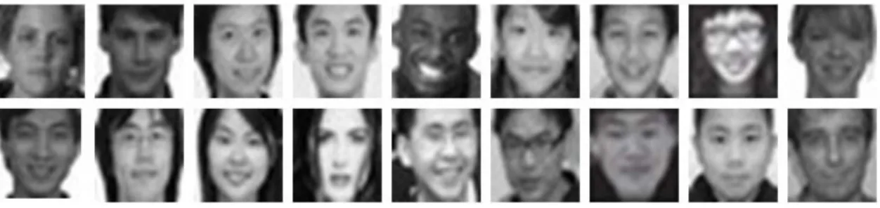
Fig. 2-10 : The positive database ... 13

Fig. 2-11 : The negative database ... 14

Fig. 2-12 : The overall classifier ... 16

Fig. 2-13 : The flow chart of training of cascaded classification ... 17

Fig. 2-14 : The flow chart of training classification for each stage ... 17

Fig. 2-15 : The image after face detecting ... 19

Fig. 2-16 : The chart of the overlapped region and the distance of a center of two blocks in (a) the local scale clustering and (b) the global scale clustering 20 Fig. 2-17 : A special case in cluster ... 21

Fig. 2-18 : (a) The results of the local scale clustering (b) the results of the global scale clustering ... 21

Fig. 3-1 : The flow chart of face identification ... 22

Fig. 3-2 : The chart of rearranging 24 X 24 pixel of image to 576 X 1 vectors ... 23

Fig. 3-3 : The average face image from our database ... 24

Fig. 3-4 : The contents of pattern information with respect to the number of eigenvectors ... 25

Fig. 3-5 : The detection rate corresponding to each number of eigenvectors ... 25

Fig. 3-6 : Example for five different head orientations of a client ... 27

Fig. 3-7 : The chart of initialization of mean vector

μ

n k, ,1 ... 29

Fig. 3-8 : The detection rate of different parameter k of the covariance matrix ... 30

Fig. 3-9 : The detection rate of different parameter

α

... 32

viii

Fig. 4-1 : (a) The results of a single face detection (b) the results of multi-faces

detection ... 34

Fig. 4-2 : The detection rate in different threshold ... 35

Fig. 4-3 : The numbers of false accept images in different threshold ... 36

Fig. 4-4 : (a), (c), (e), (g) and (i) shows the results of our face detector, Fig. 4-4(b), (d), (f), (h) and (j) shows the results of OpenCV ... 37

Fig. 4-5 : The performance of face identifier with respect to the number of clients ... 41

Fig. 4-6 : The performance of adaptive updating ... 42

Fig. 4-7 : The threshold distinguishing the clients and impostors ... 43

Fig. 4-8 : The testing result generated from the proposed face identifier. (a) The results of a single person (b) the results of multi-persons ... 44

Fig. 4-9 : The overview of clients ... 45

Fig. 4-10 : The result of face identifier ... 45

Fig. 4-11 : (a)~(e) present the procedures of capturing five images ... 47

Fig. 4-12 : The overview of updated clients ... 47

Fig. 4-13 : The result of registering client of face identifier ... 48

Fig. 4-14 : Examples of system fail #1 ... 49

Fig. 4-15 : Examples of system fail #2 ... 49

1

Chapter 1

Introduction

1.1 Motivation

Biometrics is an emerging technology for identifying people by their physical and/or behavioral characteristics [1], [2], and its applications play an important role recently. The physical characteristics of an individual that can be used in biometric identification/verification systems are fingerprint, palmprint, face, and ear; the behavioral characteristics include signature, speech, gesture, and gait. Among all biometric identification methods, face recognition has attracted much attention in recent years. Furthermore, face recognition owns the benefit of being a passive and non-intrusive system for verifying personal identity.

A typical face recognition system is composed of two parts: face detection and face identification. The purpose of face detection for the recognition system is to localize and extract the face region from the background. Following the face detection, pattern recognition methods are employed to identity the extracted face. Hence, a complete face recognition system can locate the region of faces and identify personal identity for these faces.

Many researches of face recognition focus on identifying the face without the function of detecting faces. These do not work in this situation which is not locating the face from images. Most of presented works lack resilience to add client automatically that are not sufficient for many real-time tasks.

2

Many related works are proposed to improve either the performance of face detection or that of face identification. However, a complete face recognition system including face detector and identifier is rarely proposed in recent researches. Moreover, most of presented works lack resilience to add new clients and update clients’ information automatically. These functions are important for many real-time tasks. Hence, this work tends to propose a practical system with sufficient functions required by real-time face recognition tasks.

In this thesis, a multi–client identification system using adaptive probabilistic model (APM) is proposed to achieve a complete face recognition system which can on-line update the information of the clients. In order to improve the precision and robustness of face detection, a lighting normalization process and a region-based clustering method are applied into the proposed system. Besides, our face identification can on-line add new clients and update the clients’ information due to the design of APM. The multi – client identification system using APM has been implemented and tested based on PC. The experimental results demonstrate that the proposed system can perform well and robustly with low cost of computation load.

1.2 Related Work

The goal of a detector is to find the target which is interested by a system. It is a quite challenge for detecting the face from images, because each face has the peculiar features in truthful environment. Movement, lighting variation, orientation variation and expression variation of face effects color, luminance, shadow and contour of images possibly. For this reason, it is impossible to detect face by using a single feature. Papageorgiou [3] proposed 2D Haar feature to detect objects.. It is successful

3

in using SVM (Support Vector Machine) which is composed by training the multiple Haar features to detect face from images. Besides, Li et al. proposed a “FloatBoost” algorithm to delete the worse feature for improving the detection rate and detection speed in 2002 [6]. Liehhart and Maydt [7] proposed the extended set of Haar-like features for rapid object detection. This method increases the variety of Haar feature and enhances the precision of object detection.

Then Paul and Michael proposed three important methods to detect objects speedily in 2004 [4].

1. “Integral Image” allows the features used by detector to be computed very quickly.

2. A simple and efficient classifier based on the AdaBoost learning algorithm (Freund and Schapir [5]) for selecting a small number of features from a very large potential features.

3. A method for combining classifiers in a “cascade” which reduces the computational time, because background regions of the image can be quickly discarded.

The goal of an identifier is to identify the target in the registered database. While many approaches of face identification have been made toward identifying faces under small variations in lighting, facial expression and pose, reliable techniques for identification under extreme variations have proven elusive. The major issue in view-independent face identification is the ability to identify a registered face from different viewing directions, where the face was not seen in the past.

There are different methods for handling pose variations in face identification. These methods are typically divided into the following three major topics: 1. the invariant features methods, 2. the 3D model-based methods, and 3. the multiview

4 methods.

Invariant features methods attempt to extract features that do not change when faces are seen from novel views, and use these features to identify faces whose are, such as geometric invariants [8], [9], 10]. A disadvantage of these methods is the unfeasibility of finding sufficient number of invariant features for identification.

The 3D model-based methods focus on constructing a prototypical view from a 3D model, which is extracted from the image. A recent survey of approaches to 3D face recognition is provided in [11]. The 3D model-based methods work well for small rotation angles. However, if the rotation angle is too large, some important features will be invisible [12], and these methods will fail.

Methods based on using a number of multi-view samples are most proposed. A sufficient number of different views of a face are used to deal with the pose problem [13] in multi-view methods. Beymer [14] proposed the method of the multiview methods, which models faces with templates from 15 views, sampling different poses from the viewing sphere. The way of identification consists of two main stages, a geometrical alignment stage and a correlation stage for matching.

There are other works made to propose representation schemes that are robust to changes in viewpoint. The most famous one of such methods is the single-view eigenspaces. The concept of single-view eigenspace based on the principal component analysis (PCA; proposed in Refs. [15], [16] and popularized by Tark and Pentland [17]) was first proposed in [18].

5

1.3 Thesis Organization

The remainder of this thesis is organized as follows. Chapter 1.4 describes system architecture including system overview and system flow chart. Chapter 2 describes the process of face detection which is constructed based on AdaBoost learning algorithm. A lighting normalization and a region-based clustering method are used to improve the performance of face detection. Chapter 3 shows the identification including eigenface and adaptive probabilistic model (APM). Chapter 4 shows the experimental results of face detection and identification. Chapter 5 is the conclusion of this thesis and the future works.

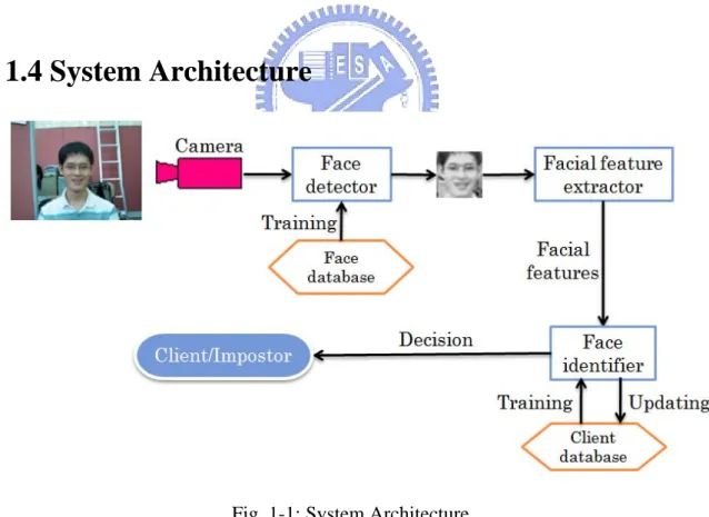
1.4 System Architecture

Fig. 1-1: System Architecture

Figure 1-1 shows the overview of our system. First, use the camera to capture the image from the scene. The face database is used to train the face detector which can

6

pick out the hypothesized faces from the image. Then, the facial feature extractor grabs the significant features from the hypothesized faces. The face identifier trained by client database can identify the hypothesized faces by their significant features. Finally, the decision of face identifier shows that they are clients or impostors.

7

Chapter 2

Face Detection

In this chapter, a feature-based system for face detection is introduced. The face detection technique employed in this system is based on the AdaBoost algorithm introduced in [4]. In the beginning, a histogram fitting method is applied for lighting normalization as a pre-process in front of the AdaBoost detector. Then, Details of using Haar-like features are described. And then, we describe the AdaBoost algorithm for combining classifiers in a “cascade.” Finally, the principle of a region-based clustering method is described.

Figure 2-1 shows the flow chart of face detection process. At the beginning of this architecture, searching windows with different scales are used to extract blocks from the images captured by a camera. The size of the searching window starts with resolution of 24 X 24 (pixels). Images with 384 X 288 pixels are scanned by 12 scales of searching windows with a scaling factor of 1.25. Then, the size and luminance of the extracted block is normalized to the same. A face detector trained by face database detects the face from the normalized block. Finally, a region-based clustering method is proposed to precisely locate the face regions from the image.

8

9

2.1 Lighting normalization

Before extracting facial features, a lighting normalization method using histogram fitting [20] is applied. In this process, a target histogram function (G l ,

( )

l=0,1, 2,..., 255; where l is the discrete gray-scale intensity level) is chosen as the histogram of the image closest to the mean value of the face database. The primary task of histogram fitting is to transform the original histograms of extracted blocks (described with a histogram function H l ) to be the same as the target

( )

histogram (described as G l ).

( )

The detail of histogram fitting is described as follow: At the beginning, have to find the functions M_H→U

( )

l (Eq. (2.1)) and M_G→U

( )

l (Eq. (2.2)) that map the histograms H l and

( )

G l onto a uniform distribution histogram. Figure 2-2 and

( )

Fig. 2-3 shows the expression of mapped histogram by Eq. (2.1) and Eq. (2.2).

( )

( )

( )

0 1 0 l j H U L j H j M l H j = → − = =

∑

∑

(2.1)

( )

( )

( )

0 1 0 l j G U L j

G j

M

l

G j

= → − =

=

∑

∑

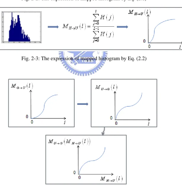
(2.2)

In order to find the desired mapping function M_H→G

( )

l that maps the image histograms onto the target histograms. Need to find the function of M_U→G

( )

l which is the inverse function of M_G→U

( )

l . Then, the desired mapping function M_H→G

( )

l

10

can present as Eq. (2-3). Figure 2-4 shows the transformed process of desired mapping function by Eq. (2-3).

( )

(

( )

)

, 0,1,..., 1 H G U G H U

M _→ l =M _→ M _→ l l= L− (2.3)

Fig. 2-2: The expression of mapped histogram by Eq. (2.1)

Fig. 2-3: The expression of mapped histogram by Eq. (2.2)

11

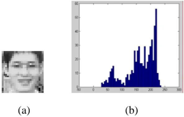
Figure 2-5(a) is the chosen target image and (b) is the histograms of the chosen target image. The origin histograms of transformed images are shown in Fig. 2-6(a) and (b) are the histograms of transformed images after the histogram fitting.

(a) (b)

Fig. 2-5: (a) The chosen target image (b) the histograms of the chosen target image

(a)

(b)

Fig. 2-6: The histograms of transformed images (a) before and (b) after the histogram fitting

12

2.2 Features

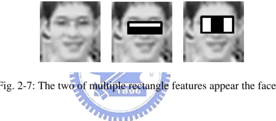
The features used in this work are reminiscent of Haar basis functions which have been used by Papageorgiou [3]. It is feasible to use composition of multiple different brightness rectangles to present the light and dark region in the image. If we can know the entire rectangle features which present the target object, the target object can be detected by contrasting unknown objects with the rectangle features. For characteristic of faces, the difference in intensity between the region of the eyes and a region across the upper cheeks is shown in Fig. 2-7.

Fig. 2-7: The two of multiple rectangle features appear the face

We use four kinds of rectangle features which are shown in Fig. 2-8.

Fig. 2-8: The four kinds of rectangle features

valve_subtracted = f x y w h Type

(

, , , ,

)

(2.4)

13

coordinate of rectangle features in the searching window. The searching window is used to find the block which has a face inside in the image. The significance of w, h denotes the relative weight and height of rectangle features. Type presents which kinds of rectangle features. valve_subtracted is the sum of the pixels in white rectangle subtracted from dark rectangle.

A single rectangle feature which best separates the face and non-face samples can be considered as a weak classification. That is, for each rectangle feature, the weak classification determiners the optimal threshold classification function, such that the minimum number of examples are misclassified.

The threshold selection for rectangle features is described below. Figure 2-9 is the flow chart of threshold selection for rectangle features.

Fig. 2-9: The flow chart of selecting threshold for rectangle features

14

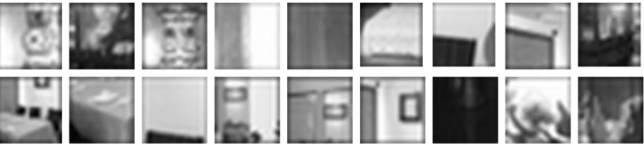
Fig. 2-11: The negative database

Selected threshold of a rectangle feature is trained by lighting normalized face database which consists of 4,000 face images and 59,000 non-face images. Figure 2-10 and Figure 2-11 present the positive and negative database. In this procedure, we need to collect the distribution information of subtracted values by this rectangle feature for face database. Then, find a threshold which discriminates the two classes to make detection rate higher than others. Eq. (2.5) is a weak classifier h x f p

(

, , ,θ

)

consists of a feature f x y w h type , a threshold

(

, , , ,

)

( )

θ and a polarity

( )

p indicating the direction of inequality. x indicates a 24 X 24 pixels sub-window of an image.

(

, , ,

)

1,

( )

0, if pf x p h x f p otherwise θ θ _{= ⎨}⎧⎪ < ⎪⎩ (2.5)

15

2.3 Training of detector

For the minimum resolution of the detector, which is 24 X 24, the exhaustive set of rectangle features are quite large, 160,000. Even through each rectangle feature can be computed very efficiently, computing the complete set is prohibitively expensive. Viola [4] presents a variant of AdaBoost is used both to select the rectangle features and to train the classifier. In its origin form, the Adaboost learning algorithm is used to boost the classification performance of a single learning algorithm. It does this by combining a collection of weak classification functions to form a stronger classifier.

In their results, the stronger classifier consists of 200-rectangle features provides initial evidence that a boosted classifier constructed from rectangle features is an effective technique for face detection. However the performance of computation time of stronger classifier is not good so that it is not sufficient for many real-world tasks.

A structure of cascaded classifiers which achieves increased detection performance while radically reducing computation time is proposed by Viola [4]. The related researches of extended structures of cascaded classifiers are introduced in the after. In our thesis, we train the classification with the concept of a structure of cascaded classifiers.

The overall classifier is shown in Fig. 2-12 that is composed of many classifiers of stages. Stages in the cascade are constructed by training classifiers using AdaBoost. In stage1, an object extracted by searching window is classified as face so that it is allowed entering to stage2, otherwise the object is rejected. As same as in stage3 the object has to pass by stage2. In brief, a labeled face is passed through a series of stages, a rejected object is rejected by particular stage even if it enters the last stage.

16

Fig. 2-12: The overall classifier

The cascade design is driven from a set of detection and performance goals. The number of cascade stages must be sufficient to achieve excellent detection rate while minimizing computation. For example, if each stage has a detection rate of 0.99 (since

10

17

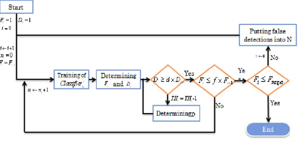
Fig. 2-13: The flow chart of training of cascaded classification

The flow chart of training of cascaded classification is shown in Fig. 2-13. The value for f is the maximum acceptable false positive rate each stage, d is minimum acceptable detection rate each stage, F_{target is overall false positive rate, P is the set}

of face samples, and N is the set of Non-face samples. The meaning for i is the stage of cascaded classification and n is the number of weak classification in the stage. _i The overall false positive rate must be smaller than F_{target and each stage have to}

satisfy the equality: F_i ≤ ×f F_i−1.

Fig. 2-14: The flow chart of training classification for each stage

The classifiers for stages in the cascade are constructed by training classifiers using AdaBoost. The procedure of this is shown in Fig. 2-14. m and l are the

18

number of non-faces and faces respectively, j is the sum of non-faces and faces samples. First we have to initialize weights _, 1 , 1 0,1

2 2

i j j

w for y

m l

= = respectively, normalization the weights by Eq. (2.6). Then, according to Eq. (2.7) select the best weak classifier with respect to the weighted error.

, , , 1 i j i j n i k k w w w = ←

∑

(2.6)

(

)

, , , min , , , i f p i j j j j w h x f p y θ ε =

∑

θ − (2.7)

Defining the h x f p

(

, , ,θ

)

while we find the best weak classifier and updating the weights by Eq. (2.8), where e_j = 0 if samples x_j is classified correctly, e_j = 1 otherwise, and 1 i i i ε β ε =

− . Eq. (2.9) and Eq. (2.10) is the final classifiers of the stage.

1 , , j e i j i j i w ←w β − (2.8)

( )

1, , , ,

(

)

1 2 0, i j i j h x f p C x otherwise α θ α ⎧ _≥ ⎪ = ⎨ ⎪⎩ (2.9) Where 1 log i i α β = (2.10)

19

2.4 Post-process: A region-based clustering method

The face detector can find a lot of candidates around faces in a scanned image as shown in Fig. 2-15.

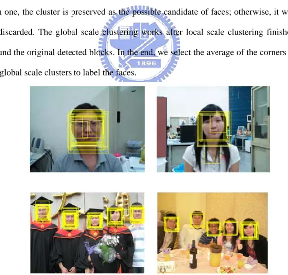
Evidently, we need to deal with the troubled problem that more than two blocks are classified as faces around a single face. A region-based clustering method is proposed to solve this problem. The method consists of two levels of clustering, one is called local scale clustering and another is called global scale clustering. The local scale clustering is used to cluster the same scale of blocks and design a simple filter to judge numbers of blocks in clusters. While numbers of blocks in a cluster are more than one, the cluster is preserved as the possible candidate of faces; otherwise, it will be discarded. The global scale clustering works after local scale clustering finished around the original detected blocks. In the end, we select the average of the corners in the global scale clusters to label the faces.

20

( )

, 1 1

( )

2

( )

0 if and cluster x y otherwise ⎧⎪ = ⎨ ⎪⎩ 　 (2.11)

( )

_

(1) _overlap rate x y, ≥TH_{overlap rate}

(2.12)

( )

(2) ,distance x y ≤TH_distance

(2.13) Eq. (2-11), Eq. (2.12) and Eq. (2.15) are formulated decision rules of the proposed method. cluster x y

( )

, = means the block x and 1 y are in the same cluster and their bounding regions is overlapped. overlap rate x y is the _

( )

, percentage of overlapped region for _{x and} y, distance x y

( )

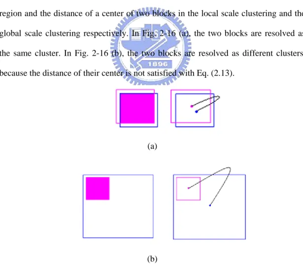
, is the distance of a center for _{x and} y. Figure 2-16 (a) and (b) shows the chart of the overlapped region and the distance of a center of two blocks in the local scale clustering and the global scale clustering respectively. In Fig. 2-16 (a), the two blocks are resolved as the same cluster. In Fig. 2-16 (b), the two blocks are resolved as different clusters, because the distance of their center is not satisfied with Eq. (2.13).

(a)

(b)

Fig. 2-16: The chart of the overlapped region and the distance of a center of two blocks in (a) the local scale clustering and (b) the global scale clustering

21

The two blocks are not in the same cluster in Fig. 2-16(b). In a special case as shown in Fig. 2-17, the four blocks are in the different clusters. Therefore, they are considered as faces and located in the image; the most of them are false accept blocks. For the reason, we choose the one of them block to replace the others if they are satisfied with Eq. (2.12).

Fig. 2-17: A special case in cluster

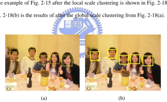
The example of Fig. 2-15 after the local scale clustering is shown in Fig. 2-18(a) and Fig. 2-18(b) is the results of after the global scale clustering from Fig. 2-18(a).

(a) (b)

Fig. 2-18: (a) The results of the local scale clustering (b) the results of the global scale clustering

22

1

Chapter 3

Face Identification

After extracting a face from the captured image, the information of the face can be used to identify the person by the system of face identification. Two major parts of the face identification in this work are eigenfaces extraction and the adaptive probabilistic model (APM). First, we describe the details of eigenfaces extraction. Then, the proposed adaptive probabilistic model (APM) used for modeling a client’s face is presented.

The flow chart of face identification process is shown in Fig. 3-1. First, the facial feature extractor is used to extract the facial features from faces that are received from the face detector mentioned in previous chapter. The facial feature extractor is constructed by the principle components analysis (PCA) [17] which is based on projecting the image space into a low dimensional feature space. According to extracted facial features, the faces are judged as either clients or imposters by the face identifier. The face identifier is formed with the adaptive probabilistic model (APM) and the client database. Details of the proposed methods are introduced in the following sections.

23

3.1 Features

The eigenfaces technique based on principle component analysis has been widely used for pattern recognition, as well as in the field of biometrics. It is the most popular feature extraction method employed by face identification techniques [17]. The principle components analysis (PCA) techniques, also known as the Karhunen-Loeve methods, choose a dimensionality reducing projection that maximizes the scatter of all projected samples. The eigenface feature extraction based on PCA is used to obtain the most important features from the face images in our system. These features are obtained by projecting the original images into corresponding subspaces.

To begin with, we have a training set of N images, and each image consists of n elements. For example, we have N = 4000 images in our database used to compute eigenfaces. Each image has n = 24 X 24 = 576 elements. Figure 3-2 shows the chart of rearranging 24 X 24 pixel of image to 576 X 1 vectors.

Fig. 3-2: The chart of rearranging 24 X 24 pixel of image to 576 X 1 vectors

The process of obtaining a single space consists of finding the covariance matrix C of the training set and computing the eigenvectors v k_k; =1, 2,...,n . The eigenvectors v corresponding to the largest eigenvalues _k λ_k span the base of the sought subspace. Each original image can be projected into the subspace as Eq. (3.1).

24

1, 2,..., T

k vk s k m

η = ⋅Φ 　　 = (3.1) Where m ( m< ) is the chosen dimensionality of the image subspace and n

s s

Φ = Γ −Ψ , where Γ is an original images from the set of images that have to be _s projected and Ψ is the average image of the training set. In Fig. 3-3, the average image obtained from our training set is presented. The coordinates of the projected images in the subspace, η_k;k=1, 2,...,m, can be used as a feature vector for the matching procedure.

Fig 3-3: The average face image from our database

Selecting dimensionality of the image subspace is an important topic. If m is closer to n , the degree of face identification is more precise. But it spends more computational time to project the original images into the corresponding subspace. Hence, we have to choose the appropriately dimensionality of the image subspace for the precision and the computational time.

The content of pattern information with respect to the number of eigenvectors is shown in Fig.3-4. The more eigenvectors are used, the more pattern information can be expressed. Forty eigenvectors can express about 77 percentage of pattern information; fifty eigenvectors can express about 81 percentage of pattern information; sixty eigenvectors can express about 84 percentage of pattern information.

Figure 3-5 denotes the detection rate corresponding to each number of eigenvectors. While the number of selected eigenvectors is greater than twenty, the

25

degree of detection rate is not obvious improved. Instead of the number of selected eigenvectors is greater than fifty, the degree of detection rate is reduced progressively. The reason is the pattern information includes the significant information and noise. The more eigenvectors are extracted, the more noises are extracted. Hence, the performance of the detection rate is descending by the affect of the noise.

Depending on the factor of the computational load and the detection rate, we choose fifty eigenvectors as the image subspace used for face identification.

Fig 3-4: The contents of pattern information with respect to the number of eigenvectors

26

3.2 Adaptive probabilistic model (APM)

The adaptive probabilistic model (APM) is proposed to achieve a fast and functional technique of face identification. The construction of the adaptive probabilistic model (APM) is a weighted combination of simple probabilistic functions. Hence, the design of APM is sufficient for real-time tasks. Furthermore, the proposed APM can on-line register new clients and update the clients’ information. The capability of on-line registering new clients enhances the practicability of the proposed system. The detection rate of identification can also be improved by updating clients’ information for long-term usage of the proposed system.

The primary concept of the APM architecture is based on view-independent face identification. The model of view-independent face identification is constructed by five different head orientations from each person (Ebrahimpour et al. [21] proposes the model of face recognition. In the model, the face space, spanning from right to left profiles along the horizontal plane, is divided into five views). The view-independent model of face identification is more robust than the single view model, because the head orientation of a person is variable in real world.

Our model is designed to achieve view-independent face identification with a mixture of view-independent faces modeled by probabilistic functions. The view-independent model of face identification is constructed by five different head orientations from each client as shown in Fig. 3-6.

27

Fig 3-6: Example for five different head orientations of a client

3.2.1 Similarity measure

APM follows probabilistic constraint, that is, similarity measures of APM are designed to model the likelihood functions. The judgment of classification is relying on the degree of likelihood. For example, the similarity of a testing sample

x

between each registered client is computed with the likelihood functions of each client. Then, the testing sample x is classified as the client corresponding to the biggest similarity.

The likelihood function APM_n

( )

x for class n is a mixture of probabilistic functions. P_{n k,}

( )

x k; =1, 2,.., 5 is defined to be one of the probabilistic functions.

( )

5 , , ,

( )

1 n n k t n k k APM x w p x = =

∑

(3.2) 5 , ,1 1 1 n k k w = =

∑

(3.3)

Eq. (3.2) shows the likelihood function. In our system, n presents the label of each client, k is the one of five head orientations, and t denotes the updating times of clients’ information. The w_{n k t, ,} is the weight of each probabilistic functions, the

28 (3.4). , ,1 0.2, 1, 2,..., 5 n k w = for k = (3.4)

( )

( )

(

)

[ ]

(

)

1 , / 2 , , , , , , 1 1 1 exp 2 2 T n k d d n k t n k t n k t P x x μ x μ σ π − ⎛ ⎞⎛ ⎞ _{⎛ ⎞} =⎜_⎜ ⎟⎜_⎟⎜ ⎟_⎟ ⎜_⎝− − Σ − ⎟_⎠ ⎝ ⎠ ⎝ ⎠ (3.5)

Eq. (3.5) indicates the original probabilistic functions. d is the dimension of input vectors, μ_{n k t, ,} is the mean vector, and σ_{n k t, ,} is the covariance matrix. Due to the assumption of Eq. (3.6) (where I is the identity matrix), the probabilistic functions in Eq. (3.5) can be simplified as Eq. (3.7). Figure 3-7 indicates the chart of initial mean vector μ_{n k, ,1}.

[ ]

[ ]

1/ 2 2 , , , , 1 2 2 , , , , d d n k t n k t n k t I n k t I σ σ σ − σ − Σ = → Σ = Σ = ⋅ → Σ = ⋅ 　　 　 　 (3.6)

( )

( )

(

, ,

) (

, ,

)

, / 2 2 , , , , 1 1 exp 2 2 T n k t n k t n k d d n k t n k t x x P x μ μ σ σ π ⎛ ⎞ ⎛ ⎞⎛ ⎞ _⎜ − − _⎟ =⎜_⎜ ⎟⎜_⎟⎜ ⎟_{⎟ ⎜}− _⎟ ⎝ ⎠ ⎝ ⎠ _{⎝ ⎠} (3.7)

29

Fig 3-7: The chart of initialization of mean vector μ_{n k, ,1}

3.2.2 Parameter tuning

The magnitude of covariance matrix σ_{n k t, ,} can affect the performance of APM. For this reason, we design an experiment to find the best value of covariance matrix

, , n k t

σ form the different coefficient of covariance matrix σ_{n k t, ,} .

The face database containing images of 10 persons is used for the experiment. The database has, for each person, images of ten different head orientations. We choose five images of ten different head orientations for each person to be the training data, the other five images is used to be the testing data.

The covariance matrix σ_{n k, ,0} is initialized by the variance of training data, because the images of each person is too less to compute the variance from the images. When obtain the initialized covariance matrix σ_{n k, ,0}, we need to adjust the coefficient of covariance matrix σ_{n k, ,1}.

30 _{n k, ,1} 1 _{n k, ,0}

k

σ = ×σ (3.8)

The covariance matrix σ_{n k, ,1} is adjusted by Eq. (3.8). The detection rate with respect to different parameter k of the covariance matrix σ_{n k, ,1} is shown in Fig. 3-8. When the parameter k is larger than four and smaller than forty-three, the detection rate is obvious improved. Therefore, we choose parameter k as 5 to obtain a suitable covariance matrix σ_{n k, ,1} for APM employed in this work.

Fig 3-8: The detection rate of different parameter k of the covariance matrix

3.2.3 Adaptive updating

The topic of adaptive updating introduces the updating functions of APM. The design of adaptive updating for APM improves the detection rate of face identification. As the updating times increase, the functions of APM become more robust. The

31

model of APM will match more precisely the head orientations of the actual person While a client is identified correctly, the function of APM is updated immediately. By the design of adaptive updating for APM, we present the improvement of the detection rate in chapter 4.

(

)

(

)

, , 1 , , 1 , , n k t n k t n k t w = −α w ₋ +α M (3.9) , , 1, 0, n k t if mapped M otherwise ⎧ = ⎨ ⎩ (3.10)

The weights of each probabilistic function are adjusted using Eq. (3.9). Where α is the learning rate for the weights and

M

_{n k t, ,} is satisfied with Eq. (3.10). If

, , n k t

M is 1 for the probabilistic function, the probabilistic function is closest the test

sample. In our system, n presents the label of each client, k is the one of five head orientations, and t denotes the number of time of clients information updating. Parameters μ_{n k t, ,} and σ_{n k t, ,} for unmatched distributions remains the same. The parameters of the distribution which matched the new observation are updated using Eq. (3.11) and Eq. (3.12).

(

)

, , 1 , , 1 n k t n k t x μ = −ρ μ ₋ +ρ (3.11)

(

)

(

) (

)

2 2 , , 1 , , 1 , , , , T n k t n k t x n k t x n k t σ = −ρ σ ₋ +ρ −μ −μ (3.12)

,where ρ is the learning rate for the mean vector and the covariance matrix. The magnitude of the learning rate affects the efficiency of updating of APM. A big learning rate may cause likelihood functions of APM over fitted, so that the

32

performance of the detection rate is reduced. Nevertheless, the small learning rate has poor improving ability of the detection rate.

We use the ORL database which contains 40 persons to select the parameter α and ρ. Each person has ten images, five of them are used to be the training data, two of them are the testing data, and the others are the updating data. Figure 3-9 and Fig. 3-10 indicates the detection rate of different parameter α and ρ. Concerning the best detection rate in experiment results, we choose 0.05 to be the value of parameter α , and the value of parameter ρ _{is 0.2.}

Fig 3-9: The detection rate of different parameter α

33

Chapter 4

Experimental Results

In this chapter, experimental results of face detection and face identification are demonstrated. We implemented our system on the platform of PC with Intel P4 2.60 GHz and 1G RAM. The development tool is Borland C++ Builder 6.0 on Window XP OS. The input images are captured from camera, and all the input images are in the resolution of 320 X 240 pixels.

In section 4.1, we present the results and performance of face detection. The results and accuracy of face identification and the comparison between the proposed method and the other methods are shown in section 4.2. Furthermore, some discussions about the proposed face detector and face identifier are made in section 4.3.

4.1 Face detection

We use the features of 2D Haar and Adaboost learning algorithm to construct our face detector. Because this system is applied in eastern country, most parts of our database are eastern faces.

Figure 4-1(a) and (b) presents the results of a single face detection and the results of multi-faces detection. The yellow block indicates that the region contains a face in the image. In the case of multi-persons with different sizes of faces, the face detector can precisely allocate regions of the faces from the image.

34 (a)

(b)

Fig. 4-1: (a) The results of a single face detection (b) the results of multi-faces detection

Table 1: The comparison between face detectors with and without lighting normalization

35

We design an experiment for the performance of face detector by estimating the detection rate and the numbers of false accept images. Detection rate and the numbers of false accept images are used to estimate the enhancement of lighting normalization. The test set consists of 130 pictures with 276 labeled frontal faces. Table 1 illustrates the comparison between face detectors with and without lighting normalization. Figure 4-2 and Fig. 4-3 present the detection rate and the numbers of false accept images in different threshold. We test seven different thresholds for our face detector and calculate the accuracy and the numbers of false accept images correspondingly. In our results, the performance of the face detector with lighting normalization is better than the face detector without lighting normalization.

36

Fig. 4-3: The numbers of false accept images in different threshold

OpenCV (Open Source Computer Vision Library Community) is an open source library. In recent years, OpenCV is widely applied to the field of image processing. One of the applications is face detection. The construction of the face detector of OpenCV also uses AdaBoost algorithm. The differences between our face detector and face detector of OpenCV are the training database and the method of post-process. Moreover, an image fitting method is employed as a lighting normalization process in our system to improve the robustness of face detection.

Figure 4-4(a), (c), (e), (g) and (i) shows the results of our face detector. Figure 4-4(b), (d), (f), (h) and (j) shows the results of OpenCV. It can be observed in Fig. 4-4 that our face detector outperforms the face detector of OpenCV, especially in cases of eastern faces.

37 (c) (d) (e) (f) (g) (h) (i) (j)

Fig. 4-4(a), (c), (e), (g) and (i) shows the results of our face detector, Fig. 4-4(b), (d), (f), (h) and (j) shows the results of OpenCV

38

4.2 Face identification

In this section 4.2, we divide the experimental results of face identification into two parts: off-line testing and on-line testing. The details of off-line testing are introduced in section 4.2.1, and the outcome of on-line testing is shown in section 4.2.2.

4.2.1 Off-line testing

Table 2 illustrates the comparison of methods and characteristics for face identification in this thesis and the other papers. The comparing methods consist of Eigenfaces, PCA+CN, SOM+CN and PCA+APM (the proposed method). Eigenfaces and PCA+CN are commonly used in pattern recognition. SOM+CN is a combined neural network (self organizing map and convolutional neural network) proposed in [22].

The comparing characteristics are based on training time, update ability, increase of clients and practicability. Because our system is based on the efficiency and performance in real time, the practicability is more important than other comparing characteristics. Our system can on-line register new clients and on-line update the information of clients in real time, hence the practicability is satisfied.

39

Table 2: The comparison of characteristics for the proposed method and the others

Table 3 presents the comparison of detection rate for our face identifier and other papers. The comparing methods similarly consist of Eigenfaces, PCA+CN, SOM+CN and PCA+APM (the proposed method). In our face identifier, a lighting normalization method is used to improve the detection rate, and the effect of this method is also demonstrated in Table 3.

The test set is ORL database which consists of 40 persons, each person has ten images. The training images for each person involves three, four and five images to model a person, the remnant images for each person are the testing images. By the different numbers of training images for each person, compare the accuracy for proposed method and the other papers.

40

Table 3: The comparison of detection rate of the proposed method and the others

The training images for our method are depending on the different head orientations to construct an APM for each person. In the comparing results, we select the optimum particular images to be training images, the rest of images in the database are testing images. Table 3 shows that the detection rate of our face identifier without lighting normalization is slightly below that of SOM+CN and higher than that of PCA+CN. The proposed face identifier with lighting normalization results in the highest detection rate.

The tolerable degree of the proposed system

In order to test the tolerable degree of our system, we design an experiment to measure the accuracy by different numbers of clients. The face database used in this experiment contains all face database used by previous experiments in this thesis, the ORL database (used in adaptive updating and the comparison with the other papers), the 10 persons database (applied in the selection of coefficient k for covariance matrix σ_{n k, ,1}) and the 13 persons database (applied in finding the threshold to distinguish the clients and impostors). There are 63 persons with 630 frontal faces used in this experiment.

41

Fig. 4-5: The performance of face identifier with respect to the number of clients

Figure 4-5 indicates the performance of face identifier with different number of clients. While the number of clients is below ten, the detection rate achieves the percentage of 100. The detection rate begins to drop off, when the number of clients exceeds ten. Until the number of clients achieves sixty-three, the detection rate is in the percentage of 86. It is accepted that the detection rate of face identifier achieves the percentage of 80. Therefore the tolerable degree of our system can accept more than sixty-three number of clients.

Adaptive updating

The ORL database is used to measure the performance of adaptive updating. We select five images for each person to be training images, three images as testing images and two images as updating images. Figure 4-6 indicates the performance of adaptive updating.

42

Fig. 4-6: The performance of adaptive updating

We use cross-validations to estimate the performance of adaptive updating. In Fig. 4-6, the upper line is the detection rate of after updating, the lower line is the detection rate of before updating. According to the results of this experiment, the face identifier with adaptive updating is obviously improved.

The threshold selection for distinguishing clients and impostors

The 26 persons’ database is used to find the threshold to distinguish the clients and impostors. We select five images for each person to be training images, and the remaining images are testing images, and the number of clients is 13. We additionally select five images from remaining 13 impostors to be testing images. The value of threshold means the value of similarity measure of APM. Figure 4-7 presents the selected threshold for distinguishing the clients and impostors.

43

Fig. 4-7: The threshold distinguishing the clients and impostors

In Fig. 4-7, FRR indicates the false reject rate and FAR indicates the false accept rate. The decreasing line is the curve of FAR and the increasing line is the curve of FRR. We utilize the intersection of FAR and FRR to be the similarity threshold. Based on the experimental result, the value of threshold for distinguishing the clients and impostors is set as 0.000125 for on-line system tested in the following section.

4.2.2 On-line testing

Results of face identification

In this part, we show the results of on-line testing. Figure 4-8(a), (b) presents the results of a single person and multi-persons generated from the proposed face

44

identifier. First, the faces are extracted from the image by the face detector, then the face identifier recognizes the faces as registered clients or impostors.

(a)

(b)

Fig. 4-8: The testing result generated from the proposed face identifier. (a) The results of a single person (b) the results of multi-persons

On-line registering new clients

The capability of registering new clients requires capturing five images of different head orientations for a new client. Figure 4-9 is the overall clients and Fig. 4-10 shows the result of face identifier. According to the overall clients, one of two persons is an impostor and the other is the client as shown in Fig. 4-10. The following section presents the procedures of on-line registering new client for the impostor in Fig. 4-10.

45

rightward and frontal faces to register the information of a new client. Figure 4-11(a)~(e) present the procedures of capturing five images. Figure 4-12 shows the overview of updated clients. Figure 4-13 shows the result after registering the new client.

Fig. 4-9: The overview of clients

46 (a)

(b)

47 (d)

(e)

Fig. 4-11: (a)~(e) present the procedures of capturing five images

48

Fig. 4-13: The result of registering client of face identifier

4.3 Discussion

For face detection, Table 1 shows that the detection rate of our face detector is more than eighty percent, and it is sufficient for a practical entrance system. The training and testing data are all frontal faces which contains many faces of eastern people.

However, there are still some situations that may cause the system fail. Figure 4-14 and Fig. 4-15 are the examples of system fail. Sometimes the shape and texture of non-faces is too close to the truly faces, the faces are non-frontal faces or partial occlusion or too small to be detected.

49

Fig. 4-14: Examples of system fail #1

Fig. 4-15: Examples of system fail #2

For face identification, Table 3 shows that the detection rate of our face identifier is more than ninety percent for the five training images for each person, and it is enough for many face identification applications. The training and testing data all consist of five images of different head orientations.

There are some situations making the system fail, such as false acceptance and false rejection. False acceptance means the impostor is identifying as the client by the face identifier; oppositely, false rejection means the client is identifying as the impostor. Figure 4-20 is an example of false acceptance , the impostor (Fig. 4-16(a)) is identified as the client (Fig. 4-16(b)).

50 (a)

(b)

51

Chapter 5

Conclusions and Future Work

In this thesis, we present a system for the multi-client identification using adaptive probabilistic model (APM). The design of this system is based on the principles of robustness and practicability.

For face detection, the technique of lighting normalization using histogram fitting is applied to improve the performance of face detector., and a region-based clustering method is proposed to deal with the problem of multi-candidates around the faces The experimental results show that the process of lighting normalization can actually improve the detection rate of face detector.

For face identification, adaptive probabilistic model (APM) is introduced to model the characteristic of the clients. According to the design of APM, the system can on-line register new clients and on-line update the information of the clients. The APM is composed of five images of different head orientations for each person. By the process of adaptive updating, the weights of five different poses and the matched probabilistic function are adjusted to adapt the latest information of registered clients.. The experimental results show that the proposed APM technique actually has the good performance for face identification.

To further improve the performance and the robustness of our system, some enhancements can be done in the future:

(a) A robust face detector is necessary for a practical face recognition system. If the faces are not extracted from the images correctly, the face identifier cannot work in the following process. For our system, one of the restrictions is that we cannot handle the variant poses of non-frontal faces, such as the

52

side faces. It is probably to select the variant poses of non-frontal faces be the training sets to solve this problem.

(b) It is hard to identify the face if the variation of the rotated angle for the face is too big. Before the process of face identifier, we may employ a method of face calibration to deal with this problem. Furthermore, this method of face calibration can also use in face detector.

(c) For face identification, a threshold is used to discriminate between the clients and the impostors. There is a trade-off problem on the selection of the threshold. A big threshold can prevent an imposter being identified as a client, but it also increases false rejections of clients. There are two possible solutions for this problem: one is to increase the specificity of face model, the other is to apply feature extraction methods which can extract more distinguishable features than eigenfaces.

(d) The tolerable degree of the proposed system may not be affordable for requirements of large numbers of clients, for instance, an entrance guard system for a big company with hundreds of staff. Hence the tolerable degree of the identification system should be improved in the future.

(e) This work lacks quantitative results of the whole face recognition system that consist of face detection and face identification. In the future work, this kind of experiments will be designed and implemented.

53

References

[1] A. k. Jain, R. Bolle, and S. Pankanti, “Biometrics: Personal Identification in Networked Society,” eds. Kluwer Academic, 1999.

[2] D. Zhang, “Automated Biometrics: Technologies Systems,” eds. Kluwer Academic, 2000.

[3] C.P. Papageorgiou, M. Oren, and T. Poggio, “A General Framework for Object Detection,” International Conference on Computer Vision, pp. 555-562, Jan. 1998.

[4] Viola Paul and J. Jones. Michael, “Robust Real-Time Face Detection,” International Journal of Computer Vision 57(2), 137-154, 2004.

[5] Y. Freund and R. E. Schapire, “A decision-theoretic generalization of on-line learning and an application to boosting,” In Computational Learning Theory: Eurocolt 95, Springer-Verlag, pp. 23-57, 1995.

[6] S. Z. Li, Q. Zhang, H. Shum, and H. J. Zhang, “FloatBoost Learning for Classification,” Neural Information Processing Systems, 2002.

[7] Rainer Lienhart and Jochen Maydt, “An Extended Set of Haar-like Features for Raid Object Detection,” IEEE ICIP 2002, Vol. 1, pp. 900-903, 2002.

[8] P. N. Belhumeur, J. Hespanha, and D. Kriegman, “Eigenfaces vs. fisherfaces: recognition using class specific linear projection,” IEEE Trans. Pattern Anal. Mach. Intell. 17 (7) (1997) 711-720.

[9] T. F. Cootes, J. F. Edwards, and C. J. Taylor. “Active appearance models,” IEEE Trans. Pattern Anal. Mach. Intell. 23 (6) (2001) 681-685.

[10] L. Wiskott, J. M. Fellous, and C. Von Der Malsburg, “Face recognition by elastic bunch graph matching,” IEEE Trans. Pattern Anal. Mach. Intell. 19 (1997)

54 775-779.

[11] K. W. Bowyer, K. Chang, and P. Flynn, “A Survey of approaches and challenges in 3D and multi-model 3D + 2D face recognition,” Comput. Vis. Image Understanding 101 (1) (2006) 1-15.

[12] W. Zhao, R. Chellappa, A. Rosenfeld, and P. J. Phillips, “Face recognition: a literature survey,” ACM Comput. Surv. (2003) 399-458.

[13] S. Du, and R. K. Ward, “Face recognition under pose variations,” J. Franklin Inst. 343 (2006) 596-613.

[14] D. J. Beymer, “Face recognition under varying pose,” Technical Report 1461, MIT AI Lab, Massachusetts Institute of Technology, Cambridge, MA, 1993.

[15] M. Kirby, and L. Sirovich, “Application of the KL procedure for the characterization of human faces,” IEEE Trans. Pattern Amal. Mach. Intell. 12 (1) (1990) 103-108.

[16] L. Sirovich, and M. Kirby, “Low-dimensional procedure for characterization of human faces,” J. Opt. Soc. Am. 4 (1987) 519-524.

[17] M. Turk, and A. Pentland, “Eigenfaces for recognition,” J. Cogn, Neurosci. 3 (1) (1991) 71-86.

[18] A. Sehad, H. Hocini, A. Hadid, M. Djeddi, and S. Ameur, “Face recognition under varying views,” Lect. Notes Comput. Sci. 1811 (2000) 258-267.

[19] H. Murase, and S. K. Nayar, “Visual learning and recognition of 3-D objects from appearance,” Int. J. Comput, Vis. 14 (1995) 5-24.

[20] R. C. Gonzales and R. E. Woods, “Digital Image Processing,” Addison Wesley, 1993.

[21] R. Ebrahimpour, E. Kabir, M. R. Yousefi, “Teacher-directed learning inview-independent face recognition with mixture of experts using single-view eigenspaces,” Journal of the Frankin Institute 345 (2008) 87-101.

55

[22] S. Lawrence, C. L. Giles, A. C. Tsoi ,and A. D. Back, “Face Recognition : A Convolutional Neural-Network Approach,” IEEE Transaction on Neural Networks, Vol. 8, NO.1, January 1997.