基於疊代最佳化之網格參數化及其於三維著色系統之應用

全文

(1)國立交通大學資訊工程系碩士論文. 基於疊代最佳化之網格參數化及其於三維著色系統之應用 An Iterative-Optimization based Parameterization for Surface Painting Systems. 研究生：鄭仁豪指導教授：莊榮宏. 博士. 中華民國九十四年八月.

(2) 基於疊代最佳化之網格參數化及其於三維著色系統之應用 An Iterative-Optimization based Parameterization for Surface Painting Systems. 研究生 : 鄭仁豪. Student : Ren-Hao Cheng. 指導教授 : 莊榮宏博士. Advisor : Dr. Jung-Hong Chuang. 國立交通大學資訊工程學系碩士論文 A Thesis Submitted to Institute of Computer Science and Information Engineering College of Electrical Engineering and Computer Science National Chiao Tung University in Partial Fulfillment of the Requirements for the Degree of Master in Computer Science and Information Engineering August 2005 Hsinchu, Taiwan, Republic of China. 中華民國九十四年八月.

(3) 基於疊代最佳化之網格參數化及其於三維著色系統之應用. 研究生 : 鄭仁豪. 指導教授 : 莊榮宏博士. 國立交通大學資訊工程學系. 摘. 要. 三維著色為一讓使用者直接於三維表面著色之程序。著色筆觸儲存於一張由網格參數化技術產生之二維貼圖。傳統三維著色的系統，網格參數化為事先產生，此參數化平面即為三維模型之材質貼圖。在著色過程中，網格參數化是固定的，並不會根據繪圖筆觸，於顏色訊號變化較為劇烈之處給予較多的貼圖取樣。為了提高三維著色系統的效能，必須針對使用者的繪圖筆觸，於著色過程中調整網格參數化使得顏色變化劇烈的區域得到較多的貼圖取樣，且須在互動時間內完成。在這篇論文中，我們提出一個基於疊代最佳化之網格參數化架構。於互動時間內，針對顏色訊號變化較為劇烈的區域在貼圖區域上給予較多的取樣空間。. 關鍵字：網格參數化、三維著色系統、材質貼圖產生. i.

(4) An Iterative-Optimization based Parameterization for Surface Painting Systems. Student: Ren-Hao Cheng. Advisor: Dr. Jung-Hong Chuang. Department of Computer Science and Information Engineering National Chiao Tung University. ABSTRACT Surface painting is a procedure that allows the users to paint onto a surface directly. The painting strokes are stored in a texture via surface parameterization techniques. In current surface painting systems, the underlying surface parameterization is fixed during the painting process. Such a parameterization is not sensitive to the frequency spectrum of the color signal introduced by painting strokes. To associate the regions of higher color signal variation with more texture samples, we need to do the re-parameterization according to users strokes at interactive rates. In this thesis, we propose a re-parameterization scheme that is based on an iterative-optimization aiming to allocate more texture samples for regions of high signal variation and to perform at an interactive rate as well.. Keywords: surface painting, surface parameterization, texture generation.. ii.

(5) Acknowledgments. First of all, I would like to thank my advisors, Dr. Jung-Hong Chuang, for his inspirations, encouragement and guidance in the past two year. I would like to thank Dan-Chi, Wen-Zheng and Yu-Hsian for their help and advice on my work. Besides, I would like to thank Wang-Yeh and Yi-Jun’s help in my daily life for the last two years. I also appreciate all my colleagues in CGGM lab, Chih-Chun, Jong-Hon, Chi-Han, Chao-Wei, Yong-Cheng, Zheng-Li, Min-Sheng and Roger from the bottom of my heart. At last, I would like to thank my parents, my sister and my girlfriend for their support, encouragement, and love.. iii.

(6) Contents Abstract. ii. Acknowledge. iii. List of Figures. vi. List of Tables. ix. 1 Introduction. 1. 1.1. Motivation . . . . . . . . . . . . . . . . . . . . . . . . . . . . . . . . .. 1. 1.2. Contributions . . . . . . . . . . . . . . . . . . . . . . . . . . . . . . .. 3. 1.3. Thesis Organization . . . . . . . . . . . . . . . . . . . . . . . . . . . .. 3. 2 Related Work 2.1. 4. Theoretic background of parameterization . . . . . . . . . . . . . . . .. 4. 2.1.1. General setup and notation . . . . . . . . . . . . . . . . . . . .. 5. 2.1.2. First fundamental form . . . . . . . . . . . . . . . . . . . . . .. 6. 2.1.3. Some stretch metrics . . . . . . . . . . . . . . . . . . . . . . .. 9. 2.2. Mesh Parameterization . . . . . . . . . . . . . . . . . . . . . . . . . .. 10. 2.3. Surface Painting . . . . . . . . . . . . . . . . . . . . . . . . . . . . . .. 16. iv.

(7) 3 A Re-parameterization Framework for Surface Painting. 23. 3.1. Approach overview . . . . . . . . . . . . . . . . . . . . . . . . . . . .. 23. 3.2. Topological surgery . . . . . . . . . . . . . . . . . . . . . . . . . . . .. 24. 3.3. Initial parameterization . . . . . . . . . . . . . . . . . . . . . . . . . .. 27. 3.4. Stroke sampling . . . . . . . . . . . . . . . . . . . . . . . . . . . . . .. 27. 3.5. Importance map and geometry stretch map . . . . . . . . . . . . . . . .. 28. 3.6. The L2s stretch . . . . . . . . . . . . . . . . . . . . . . . . . . . . . . .. 31. 3.7. Rapid re-parameterization . . . . . . . . . . . . . . . . . . . . . . . .. 33. 3.7.1. Iterative optimization based on uniform grid . . . . . . . . . . .. 33. 3.7.2. Re-parameterization . . . . . . . . . . . . . . . . . . . . . . .. 36. 3.7.3. Stroke resampling over optimized parameterization . . . . . . .. 36. Two-stage re-parameterization framework . . . . . . . . . . . . . . . .. 37. 3.8. 4 Results and Performance Analysis. 45. 4.1. Results of surface painting . . . . . . . . . . . . . . . . . . . . . . . .. 46. 4.2. Analysis of interactive application . . . . . . . . . . . . . . . . . . . .. 47. 4.3. Signal-specialized parameterization versus our method . . . . . . . . .. 49. 4.4. Comparison to painting detail . . . . . . . . . . . . . . . . . . . . . . .. 53. 5 Conclusion and Future Work. 57. 5.1. Conclusion . . . . . . . . . . . . . . . . . . . . . . . . . . . . . . . .. 57. 5.2. Future work . . . . . . . . . . . . . . . . . . . . . . . . . . . . . . . .. 58. Bibliography. 60. v.

(8) List of Figures 2.1. Parameterization φ and embedding ψ [3]. . . . . . . . . . . . . . . . .. 5. 2.2. Γ and γ represent the largest and smallest local stretch [3]. . . . . . . .. 8. 2.3. Determine λvw for v that is inside of a triangle. . . . . . . . . . . . . .. 12. 2.4. Determine λvw for v inside a n-sided polygon [6]. . . . . . . . . . . . .. 12. 2.5. A cat head model and its harmonic map [5]. . . . . . . . . . . . . . . .. 13. 2.6. Gray-coded deformation energy of different parameterizations [11]. . .. 14. 2.7. Examples of geometric-stretch and signal-stretch parameterizations [18]. 14. 2.8. Comparison of two mesh parameterization schemes [26]. Top : Stretch minimization of Sander et al [17], Down : Yoshizawa et al. [26] . . . .. 2.9. 15. Texture mapping for a cat head model [22]. (a) cat head model. (b) ABF parameterization. (c) ABF texturing result. (d) Uniform Grid G1 . (e) Smoothed grid G2 . (f) Texturing result after applying G2 . . . . . . .. 17. 2.10 Texturing result of geometry stretch and signal stretch [18]. . . . . . . .. 18. 2.11 Each stroke is stored in an individual atlas [13]. . . . . . . . . . . . . .. 19. 2.12 Uniform mesh atlas for a cloud textured moon [1]. . . . . . . . . . . . .. 20. 2.13 Rhino sculpted from wood and its area-weighted mesh atlas [1]. . . . .. 20. 2.14 Recursively partition the mesh using Metis algorithm [1]. . . . . . . . .. 21. vi.

(9) 2.15 A multiresolution meshed atlas of a cow. Each node in the tree corresponds to (a) a cluster of triangles (b) and a square region in the texture domain. (c) Each node’s cluster is the union of its children’s clusters [2].. 22. 3.1. The overall process of our method. . . . . . . . . . . . . . . . . . . . .. 25. 3.2. Procedure of parameterizing closed-surface [3]. . . . . . . . . . . . . .. 25. 3.3. Slice the closed-mesh along the cut [3]. . . . . . . . . . . . . . . . . .. 26. 3.4. Texture domain. . . . . . . . . . . . . . . . . . . . . . . . . . . . . . .. 29. 3.5. Problems of four-tap filter. . . . . . . . . . . . . . . . . . . . . . . . .. 30. 3.6. Our filter. . . . . . . . . . . . . . . . . . . . . . . . . . . . . . . . . .. 30. 3.7. Four-tap filter and our filter. . . . . . . . . . . . . . . . . . . . . . . . .. 31. 3.8. Face model with its parameterization, geometry stretch map and importance map. . . . . . . . . . . . . . . . . . . . . . . . . . . . . . . . . .. 32. The optimization result base on one iteration. . . . . . . . . . . . . . .. 35. 3.10 Chart diagram of the optimization process. . . . . . . . . . . . . . . . .. 35. 3.11 Venus model and optimized parameterization. . . . . . . . . . . . . . .. 39. 3.9. 3.12 Parasaur model : single stage optimization using 256x256 uniform sample points . . . . . . . . . . . . . . . . . . . . . . . . . . . . . . . . .. 40. 3.13 High resolution uniform grid points. . . . . . . . . . . . . . . . . . . .. 40. 3.14 Low resolution uniform grid points. . . . . . . . . . . . . . . . . . . .. 41. 3.15 Venus model and two-stage optimized parameterization. . . . . . . . .. 42. 3.16 Parasaur model : Two-stage optimization using 16 × 16 and 256 × 256 grids. . . . . . . . . . . . . . . . . . . . . . . . . . . . . . . . . . . .. 43. 3.17 Comparison of single and two stage optimization . . . . . . . . . . . .. 44. 4.1. Painting results of the venus model. Result of a fixed-parameterization (left column) and the result of our two-stage optimized parameterization (right column). . . . . . . . . . . . . . . . . . . . . . . . . . . . . . .. vii. 47.

(10) 4.2. Back-view of the painting results of the venus model. Result of a fixedparameterization (left column) and the result of our two-stage optimized parameterization (right column). . . . . . . . . . . . . . . . . . . . . .. 4.3. 48. Painting results of the triceratops model. Result of a fixed-parameterization (left column) and the result of our two-stage optimized parameterization (right column). . . . . . . . . . . . . . . . . . . . . . . . . . . . . . .. 4.4. 49. Painting results of the face model. Result of a fixed-parameterization (left column) and the result of our two-stage optimized parameterization (right column). . . . . . . . . . . . . . . . . . . . . . . . . . . . . . .. 4.5. 50. Painting results of the face model. Result of a fixed-parameterization (left column) and the result of our two-stage optimized parameterization (right column). . . . . . . . . . . . . . . . . . . . . . . . . . . . . . .. 4.6. 51. An image is texture mapped to simulate painting strokes. Result of a fixed-parameterization (left column) and the result of our two-stage optimized parameterization (right column). . . . . . . . . . . . . . . .. 4.7. 52. Four images is texture mapped to simulate painting strokes. Result of a fixed-parameterization (left column) and the result of our two-stage optimized parameterization (right column). . . . . . . . . . . . . . . .. 54. 4.8. The optimization process of triceratops model. . . . . . . . . . . . . . .. 55. 4.9. Comparison of our result with signal specialized parameterization under different texture map resolutions. . . . . . . . . . . . . . . . . . . . . .. viii. 56.

(11) List of Tables 4.1. Statistics of initial parameterization, two-stage optimization and re-parameterization time (sec.) for four different models.. ix. . . . . . . . . . . . . . . . . . .. 53.

(12) CHAPTER. 1. Introduction 1.1 Motivation Surface painting(also called 3D painting) is a technique that allows the users to paint directly onto a 3D surface. If the discretization of the surface is fine enough, user can directly paints on the vertices of the surface. However, in general, the desired precision for the color is greater than the geometric detail of the model. Assuming that a surface is provided with a parameterization, it is convenient to store colors in the parameterized texture space. In current surface painting systems, the underlying mesh parameterization is predefined and fixed during the painting process. Such a parameterization is not sensitive to the frequency spectrum of the color signal as the result of painting strokes, and in consequence, may introduce distortion at arbitrary locations and waste texture space in areas of no stroke. Moreover, current surface painting systems parameterize the surface based only on the geometric aspects. Even though these systems provide tools allowing users to adjust the underlying parameterization, but it is not intuitive for normal users. Most surface parameterization schemes assume no prior knowledge of the signal, 1.

(13) 1.1 Motivation. 2. and take only surface’s geometry information into account. For surface painting, we want to allocate more texture samples in regions of greater signal detail by doing the re-parameterization on the fly according to the painting strokes. Moreover, the reparameterization should be fast enough to achieve an interactive rate. Sander’s signal-specialized parameterization [18] minimizes the signal stretch for a given mesh with signal information. It is, however, not suitable for surface painting since it utilizes an expensive global optimization, and cannot support the interactive reparameterization required after each stroke is painted. To support painting systems, very few methods have been proposed. In Igarashi and Cosgrove [13], painting strokes are stored as separate charts which are packed into a texture atlas. The method generates each chart such that only the region with painting strokes are included, and from which fine details can be reproduced. However, overlapping strokes made at different poses are stored in separate charts, and hence additional texture space are required. Carr et al. proposed a dynamic re-parameterization scheme based on their prior work on multiresolution meshed atlas (MMA) [1, 2]. The dynamic re-parameterization is performed by changing the so called MMA tree hierarchy. This framework is complicated and, in general, achieves better results only for the model with large polygon count. Our proposed method first derives an initial parameterization, and then, during the painting process, analyze the color signal frequency introduced by painting strokes, and utilizes an iterative optimization to do the re-parameterization to interactively allocate more texture samples for regions with high color signal variation. The proposed method is simple to implement and works well for models with either low or large polygon count..

(14) 1.2 Contributions. 3. 1.2 Contributions This thesis describes a novel and simple framework of the re-parameterization necessary for future surface painting systems. Along the way to achieve this goal, we present the following contributions: • Propose a modified signal metric L2s that measures the geometric and signal stretch of a parameterization. • Propose an interactive approach for the re-parameterization aiming to increase the sampling ratio in regions with high signal variation.. 1.3 Thesis Organization Chapter 2 introduces some background and previous works related to the thesis, including surface parameterization and surface painting. Chapter 3 presents our two-stage optimization framework for surface painting. Chapter 4 demonstrates the results of the proposed method and analyzes its performance. Chapter 5 summarizes our method and mentions some research directions..

(15) CHAPTER. 2. Related Work In this chapter, reviews on related work of parameterization and surface painting will be given.. 2.1 Theoretic background of parameterization Several schemes have been proposed that flatten a surface region and establish a parameterization over the last ten years in computer graphics. Parameterization is a mapping from a two dimension domain to a high dimension space. All previous proposed techniques explicitly aim at producing least-distorted parameterizations, and vary only in the objective function (distortion metric) and the minimization processes used. The main distinction between the functions is how they measure the difference of the resulting parameterization from an isometric one (a mapping preserving lengths and angles). In this section, we introduce several metrics that are directly related to our research.. 4.

(16) 2.1 Theoretic background of parameterization. 2.1.1. 5. General setup and notation. Before reviewing the fundamental theory, we first introduce some basic concepts and notations that are useful for introducing the fundamental theory.. Figure 2.1: Parameterization φ and embedding ψ [3]. As shown in Figure 2.1, we call ΩT ∈ R3 the surface of triangulation T and further let V = V (T ) denote the set of vertices, E = E(T ) the set of edges, and F = F (T ) the set of faces of T . If ΩT has a boundary we distinguish between the disjoint sets of interior and boundary vertices as VI and VB . Two distinct vertices v, w ∈ V are neighbors if they are the end points of an edge e = [v, w] ∈ E. For each v ∈ V , Nv = {w ∈ V : [v, w] ∈ E} denotes the set of neighbors of v. In general, parameterization φ of a triangulation T over a parameter domain ΠT ∈ R2 is a homeomorphism between this domain and the surface of T ; that is, φ : ΠT → ΩT From differential geometry, we know that such a homeomorphism and its inverse.

(17) 2.1 Theoretic background of parameterization. 6. ψ = φ−1 exist if and only if ΠT and ΩT are topologically equivalent, i.e. ΠT is a 2-manifold with the same number of boundaries and handles as ΩT . The number of handles is also called the genus of the manifold. For example, a sphere has genus zero and the genus of a torus is one, etc. If ΩT and ΠT are not topologically equivalent, some topological operations are required to change the topology of ΩT such that the result is topologically equivalent to ΠT . Most parameterizations are piecewise linear functions. Due to the piecewise linearity, ψ induces a triangulation S which is equivalent to T in the sense that vertices, edges, and triangles of S and T naturally correspond to each other; that is, ψ(V (T )) = V (S), ψ(E(T )) = E(S), ψ(T ) = S, and φ(V (S)) = V (T ), φ(E(S)) = E(T ), φ(S) = T. We call triangles of S parameter triangles and S itself the parameter triangulation. Note that φ and ψ are uniquely determined by the images ψ(v), which we call the parameter points or parameter values of the vertices v ∈ V . Hence the task of parameterizing T amounts to finding parameter values ψ(v) ∈ ΠT , one for each vertex v ∈ V . Since we also expect ψ to be bijective, we have to assure that the parameter points are arranged such that the parameter triangles do not overlap or flip (adjacent triangles in ΩT with opposite orientation).. 2.1.2. First fundamental form. In this section, we introduce more complicated metrics of parameterizing ΩT based on the first fundamental form from differential geometry. Given a differentiable surface Ω and its parameterization φ, we can regard the parameterization φ as a mapping from R2 to R3 by φ(u, v) = [x(u, v), y(u, v), z(u, v)].

(18) 2.1 Theoretic background of parameterization. 7. with the following differential forms ∂x ∂x dv, du + ∂v ∂u ∂y ∂y dv, du + dy = ∂v ∂u ∂z ∂z dv. du + dz = ∂v ∂u. dx =. We define the line element as dl2 = dx2 + dy 2 + dz 2 or alternatively, dl2 = E(u, v)du2 + 2F (u, v)dudv + G(u, v)dv 2 ,. (2.1). where µ ¶2 µ ¶2 µ ¶2 ∂z ∂y ∂x ∂φ , + + = · ∂u ∂u ∂u ∂u µ ¶ µ ¶ µ ¶ µ ¶ µ ¶ µ ¶ ∂z ∂z ∂y ∂y ∂x ∂x ∂φ , · + · + · = · ∂v ∂u ∂v ∂u ∂v ∂u ∂v µ ¶2 µ ¶2 µ ¶2 ∂z ∂y ∂x ∂φ ∂φ . + + = · G(u, v) = ∂v ∂v ∂v ∂v ∂v. ∂φ E(u, v) = ∂u ∂φ F (u, v) = ∂u. E(u, v)du2 + 2F (u, v)dudv + G(u, v)dv 2 in Equation 2.1 is known as the the first fundamental form which determines the arc length of a curve on the surface. Arranging the coefficient in a symmetric matrix form  I=.  E F F G. we have ³. ´. , . . dl2 = du dv I . du dv. .. The matrix I is called the metric tensor, which can be decomposed as I = JT J where. ·. ∂φ ∂φ , J= ∂u ∂v. ¸.

(19) 2.1 Theoretic background of parameterization. 8. is the Jacobian matrix of φ. We can show that if Γ and γ are singular values of J, Γ2 and γ 2 will be eigenvalues of I. Since J can be seen as a local affine mapping from R2 to R3 , denoted by   ³ ´ p q = J o  , 1. q, o ∈ R3 ,. p ∈ R2 ,. where o is the original point for completing the affine mapping, it is intuitive to use Γ and γ for describing the lengths and angles of vectors in R2 after being mapped by φ. In other words, the singular values Γ and γ represent the largest and smallest length obtained after mapping unit-length vectors from R2 to R3 , i.e. Γ and γ can represent the largest and smallest local “stretch” of φ.. Figure 2.2: Γ and γ represent the largest and smallest local stretch [3]. Because triangulated surface ΩT is piecewise linear, φ can be seen as the piecewise linear map f as shown in Figure 2.2. The common way to represent f is the barycentric mapping B(p) defined as B(p) = (< p, p2 , p3 > q1 + < p, p3 , p1 > q2 + < p, p1 , p2 > q3 )/ < p1 , p2 , p3 > where < a, b, c > denotes the area of 4abc and p is a point on the 4abc. We can.

(20) 2.1 Theoretic background of parameterization discretize J and denote it as JT  ∂x/∂u JT =  ∂x/∂v. 9. t ∂y/∂u. ∂z/∂u. ∂y/∂v. ∂z/∂v. t. .  =. ∂B/∂u. . ∂B/∂v. where ∂B/∂u = Bu = (q1 (v2 − v3 ) + q2 (v3 − v1 ) + q3 (v1 − v2 ))/(2A) ∂B/∂v = Bu = (q1 (u3 − u2 ) + q2 (u1 − u3 ) + q3 (u2 − u1 ))/(2A) and A =< p1 , p2 , p3 >= ((u2 − u1 )(v3 − v1 ) − (u3 − u1 )(v2 − v1 ))/2 Thus the Jacobian matrix of ΩT is    (v2 − v3 ) (u3 − u2 ) x1 x2 x3   1     JT =  y y y  (v − v1 ) (u1 − u3 ) 2A  1 2 3   3  (v1 − v2 ) (u2 − u1 ) z1 z2 z3 and the largest and smallest singular values of JT are given respectively by r ´ ³ p 2 2 Γ = 1/2 (a + c) + (a − c) + 4b , r ´ ³ p γ = 1/2 (a + c) − (a − c)2 + 4b2 . where a = Bu · Bu , b = Bu · Bv , and c = Bv · Bv .. 2.1.3. Some stretch metrics. Based on above deduction, various stretch metrics base on the versatile Γ and γ have been proposed. For example, Sander et al. [17] define an L2 distortion measure by taking the root-mean-square of Γ and γ, and define L∞ as the largest singular value Γ: q 2 2 2 L = Γ +γ 2 L∞ = Γ.

(21) 2.2 Mesh Parameterization. 10. Hormann et al. [11] defines a deformation metric as Ld =. Γ γ + γ Γ. Sorkine et al. [24] defines a geometric distortion as ¾ ½ 1 Lg = max Γ, γ Khodakovsky et al. [15] defines an area distortion as Larea = Γ · γ and an anisotropic distortion as Langle =. Γ γ. 2.2 Mesh Parameterization Over the last years, a lot of research has been done in the area of surface parameterization. In the context of parameterization, harmonic maps were first used by Eck et al. [5]; see Figure 2.5. However, the texture coordinates for boundary vertices must be fixed a prior and harmonic maps may contain face flips, which violate the bijectivity of the parameterization. Based on earlier work by Tutte [25], Floater proposed a specific weight based on the barycentric maps to obtain a mapping that is shape-preserving [6]. It guarantees the embedding for convex boundaries and find a parameterization by solving a linear system. The first step of the method is to specify the parameter points ψ(v) of the boundary vertices v ∈ VB . Then, set each interior vertex v ∈ VI to be a convex combination of its neighbors. For each interior vertex v, a set of strictly positive convex weights λvw , w ∈ Nv , is chosen such that. X w∈Nv. λvw = 1..

(22) 2.2 Mesh Parameterization. 11. For all interior vertices, the mapping ψ(v), v ∈ VI , is determined by solving the following linear system of equations: ψ(v) =. X. λvw ψ(w),. v ∈ VI .. w∈Nv. This equation can be rewritten as ψ(v) −. X. X. λvw ψ(w) =. λvw ψ(w),. v ∈ VI ,. w∈Nv and w∈VB. w∈Nv and w∈VI. and further as Bx = c. The problem remained is how to determine the value of λvw . There are two cases needed to be discussed. The first case is that v is inside of a triangle as shown in Figure 2.3. We can represent v as v=. area(v, w3 , w1 ) area(v, w2 , w3 ) area(v, w1 , w2 ) · w2 , · w1 + · w3 + area(w1 , w2 , w3 ) area(w1 , w2 , w3 ) area(w1 , w2 , w3 ). and then set. area(v,w2 ,w3 ) λvw1 = area (w1 ,w2 ,w3 ) area (v,w3 ,w1 ) λvw2 = area(w 1 ,w2 ,w3 ) area (v,w1 ,w2 ) λvw3 = area(w1 ,w2 ,w3 ). The second case is that v has more than three neighbor vertices. As shown in Figure 2.4, since 4w1 w4 w5 encloses v, we can solve λvw1 , λvw4 and λvw5 using the previous method. Similarly, for each triangle k that has an end point wi and encloses v, we compute λkvwi and set λvwi as λvwi =. 1X k λ d k vwi. where d is the degree of v. Floater later proposed an improved method, called mean value coordinates, which derives the weights by using the mean value theorem [7]. The method also guarantees.

(23) 2.2 Mesh Parameterization. 12. Figure 2.3: Determine λvw for v that is inside of a triangle.. Figure 2.4: Determine λvw for v inside a n-sided polygon [6]. the existence of bijective mapping and is faster than the shape-preserving parameterization. Desbrun et al. defined a space of measures spanned by a discrete version of the Dirichlet energy and a discrete authalic energy [4]. While the authalic energy remedies.

(24) 2.2 Mesh Parameterization. 13. local area deformations, it requires fixed boundaries and, moreover, produces results that are no better than the one computed by the parameterization using global length preservation.. Figure 2.5: A cat head model and its harmonic map [5]. Hormann and Greiner proposed MIPS (Most Isometric Parameterizations) algorithm, which attempts to preserve the ratio of singular values over the parameterization using a hierarchical solver [11, 12]. The method finds a parameterization with “natural boundary” that minimizes the highly non-linear stretch metric. Figure 2.6 shows the MIPS parameterization with natural boundary. However, the metric disregards absolute stretch scale over the surface. As a result, a small domain area can map to a large region on the surface. Sander et al. proposed a non-linear stretch that integrate the sum of squared singular values over the map. We refer to this metric as geometric stretch. The parameterization is derived by a coarse-to-fine optimization scheme that minimizes the geometric stretch over the map. Note that the resulting parameterization may encounter parametric crack problem. Sander et al. developed a signal-stretch metric that combines both surface area and surface signal bandwidth [18]. It is shown that the stretch metric is related to SAE.

(25) 2.2 Mesh Parameterization. (a) Most Isometric Parameterization. 14. (b) Discrete Harmonic Parameterization. Figure 2.6: Gray-coded deformation energy of different parameterizations [11]. (Signal-Approximation Error) - the difference between a signal defined on the surface and its reconstruction. Sander’s signal stretch can be seen as the extension of the geometry stretch. Figure 2.7 shows the results of the parameterization using geometric-stretch and signal-stretch parameterizations.. (a) Geometric-stretch parameterization. (b) Signal-specialized parameterization. Figure 2.7: Examples of geometric-stretch and signal-stretch parameterizations [18]. Parameterization using either geometric stretch or signal stretch involves a process of expensive non-linear optimization. Yoshizawa et al. developed a simple and fast method that computes the parameterization of low geometry stretch [26]. Floater’s shape preserving parameterization [6] is used as an initial parameterization, which is then optimized gradually. At each step, the parameterization generated at previous step is optimized by updating the set of positive convex weights λvw for each interior vertex.

(26) 2.2 Mesh Parameterization. 15. v ∈ VI using geometry stretch. The formula is as follows: λnew vw =. λold vw , σw. w ∈ Nv. where σw =. qX. σ(U ) =. p. A(Tu )σ(Uu )2 /. (Γ2 + γ 2 )/2,. X. A(Tu ),. U = hu1 , u2 , u3 i in the parametric plane,. and A(Tu ) is the area of triangle Tu and the sums are taken over all triangles Tu surrounding the vertex. After the weights are updated, the new parameterization is computed by solving a linear system, which is fast. Moreover, the parametric cracks that may happen in Sander’s global optimization will not be encountered. This method is, however, heuristic and lack of rigorous mathematical support. Nevertheless, it is fast and powerful for generating parameterization with low geometry stretch. See Figure 2.8 for the comparison.. Figure 2.8: Comparison of two mesh parameterization schemes [26]. Top : Stretch minimization of Sander et al [17], Down : Yoshizawa et al. [26] Another approach that minimizes angular distortion is proposed by Sheffer and Sturler [21]. The parameterization is derived by minimizing the relative distortion of the.

(27) 2.3 Surface Painting. 16. planar angles with respect to their counterparts in the three-dimensional space. Though the minimization problem is linear, it becomes non-linear as some other non-linear constraints have to be taken into account in order to generate a valid solution. As a type of discrete conformal parameterization, the method suffers more area distortion, especially in region closed to the center of the surface. The area distortion leads to linear distortion in texture mapping. Sheffer et al. tried to solve the problem by applying a mesh smoothing procedure to the uniform grid overlaying on the parametric domain [22]. The smoothing uses a sizing function which is based on the ratios between the lengths of the edges in the three-dimensional surface and their counterparts in parametric domain. Figure 2.9 demonstrates the result of texture mapping by overlaying a regular grid. Levy et al. computed quasi-conformal parameterizations by measuring the violation of the Cauchy-Rieman equation in the least square sense [16]. They also show that the quasi-conformal parameterization exists uniquely, independent of resolution and preserves orientations. Using a standard numerical conjugate gradient solver they are able to compute least squares approximations to continuous conformal maps very efficiently without requiring fixed boundary texture coordinates.. 2.3 Surface Painting Surface painting system allows users to paint directly onto a three-dimensional surface and stores the painting result in a texture. The mapping between mesh and texture space is built via a parameterization. In current surface painting systems, the parameterization is pre-computed and remains fixed during the painting process. One and the only thing done by surface painting systems is to sample painting stokes into the texture space. In this way, it is often that insufficient samples will be found in the regions with high painting detail. The left side of Figure 2.10 shows that the aliasing occurs in the region.

(28) 2.3 Surface Painting. 17. Figure 2.9: Texture mapping for a cat head model [22]. (a) cat head model. (b) ABF parameterization. (c) ABF texturing result. (d) Uniform Grid G1 . (e) Smoothed grid G2 . (f) Texturing result after applying G2 . spaced in-between black and white. The right part of Figure 2.10 depicts same model with reduced aliasing, as the result of using a parameterization that takes the signal variation into account. Hanrahan and Haeberli firstly proposed the concept of three dimensional surface painting, in which the color signal is stored directly in mesh vertices [10]. Based on this method, the shading result is interpolated between mesh vertices, though we could not reveal rich texture detail. Igarashi and Cosgrove stored the paint strokes image that occurred for each pose as separate charts packed into a texture atlas [13]. As shown in Figure 2.11, the eyes and mouth were first painted. Mesh triangles affected by these strokes are found and.

(29) 2.3 Surface Painting. 18. Figure 2.10: Texturing result of geometry stretch and signal stretch [18]. projected onto a two dimensional domain to form an atlas. Similarly, each subsequent stroke is stored in a new atlas. When the painting process complete, all the atlas are packed together to form the final texture atlas. The major disadvantage of the method is that a stroke that overlapping other strokes may appear in more than one atlas; as shown in Figure 2.11. In such cases, texture space may be wasted. Before going on the approach proposed by Carr et al., we address the concept of procedural texturing. The simplest form of texturing is texture mapping. The texture space is usually created from an image file, often a photograph or artist’s rendering of the material. The major disadvantage is that aliasing occurs when the texturing is under.

(30) 2.3 Surface Painting. 19. Figure 2.11: Each stroke is stored in an individual atlas [13]. either minification or magnification. Another issue is that the mapping function itself could be complicated. The essential idea of procedural texturing is that the color of a pixel is based functionally on the three dimensional coordinates of its corresponding vertex. In general, the result of procedural texturing is stored via texture atlases. Some methods for constructing mesh atlas have been proposed, for example, uniform mesh atlas (Figure 2.12), area-weighted mesh atlas (Figure 2.13) and length-weighted mesh atlas. There are two major drawbacks among these methods. The first is that the texture sample space is not completely used. As shown in Figure 2.13, much texture space are wasted at the right-side of the atlas. The second drawback is that these methods do not take the triangles’ shape and area into account. As shown in Figure 2.12, each triangle has the same sample space no matter how large it is. Carr and Hart made use of the Metis algorithm [14] to recursively partition the mesh into several charts; see Figure 2.14. A quaternary tree hierarchy, called MMA, is then constructed. The construction is based on the clustering of charts via a top-down or a bottom-up approach. The MMA framework takes the size of mesh triangles into account such that each triangle could be allocated suitable texture sample space..

(31) 2.3 Surface Painting. 20. Figure 2.12: Uniform mesh atlas for a cloud textured moon [1].. Figure 2.13: Rhino sculpted from wood and its area-weighted mesh atlas [1]. Based on the MMA framework, Carr and Hart proposed a method aiming to derive a parameterization that is sensitive to signal distribution [2]. The method consists of three steps. Firstly, the mesh is divided into several charts based on the method proposed by Sander et al. [19]. Several triangles are chosen as seed of the charts and from each of which faces are joined into chart based on the geometric distance and normal difference between face and chart. Secondly, each chart is parameterized into a two.

(32) 2.3 Surface Painting. 21. Figure 2.14: Recursively partition the mesh using Metis algorithm [1]. dimensional domain based on Sander et al’s geometry stretch metric [17]. Finally, an MMA hierarchy is constructed for all charts built in step one. Each chart has the weight as its L2 stretch computed in step two. The MMA hierarchy can be presented by a quaternary tree, in which tree nodes at the same level have the same weight, and, in consequence, have equivalent texture space. As shown in Figure 2.15, each of the four child nodes occupies one-fourth texture space of its parent node. During the surface painting process, all painting strokes are rendered into texture and then the stroke frequency distributed on the texture is analyzed using graphics hardware. After the analysis, an importance value computed from frequency analysis for previous strokes is attached to each chart and the MMA hierarchy(quaternary tree) is re-balanced to generate a new parameterization. All of the charts are placed in a priority queue based on the importance value. The MMA hierarchy is reconstructed via the priority queue. Each chart should consist of a quite large number of faces in order to reduce distortion introduced by the parameterization. Moreover, the re-balancing is more significant with more number of charts. Therefore this method is suitable for meshes with large number of triangles..

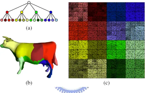
(33) 2.3 Surface Painting. 22. Figure 2.15: A multiresolution meshed atlas of a cow. Each node in the tree corresponds to (a) a cluster of triangles (b) and a square region in the texture domain. (c) Each node’s cluster is the union of its children’s clusters [2]..

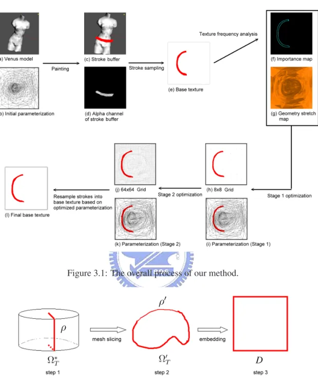
(34) CHAPTER. 3. A Re-parameterization Framework for Surface Painting 3.1 Approach overview To optimize the sampling resolution in parametric space, our basic idea is to increase the resolution of regions with high signal variation while decreasing the resolution of other regions. Our parameterization optimization framework for surface painting comprises the following steps as shown in Figure 3.1: 1. Transform the closed-surface Ω∗T into an open-surface Ω0T using topological surgery, construct a global initial parameterization for the surface mesh, and generate a base texture based on the parameterization. 2. Resample painting strokes into the base texture. Analyze the signal frequency on base texture using graphics hardware to generate the importance map. Another 23.

(35) 3.2 Topological surgery. 24. map called geometry stretch map is also computed using graphics hardware. 3. Apply a uniform grid G underlying the parameterization domain, in which each point of G is assigned a L2s stretch value derived from importance map and geometry stretch map, and then apply a two-stage optimization to get an optimized uniform grid Gopt . 4. Re-parameterize Ω0T according to the optimized uniform grid Gopt , and resample the painting strokes according to the new parameterization. Our proposed parameterization optimization framework has the following characteristics: • Topological surgery is used to automatically transform the closed-surface into an open-surface which is topologically equivalent to a disk. • A method which analyzes the surface signal variation by using graphics hardware. • A re-parameterization derived based on optimized uniform grid approach is fast enough for interactive applications.. 3.2 Topological surgery To parameterize ΩT onto a planar domain, ΩT should be topologically equivalent to a disk. If ΩT is a closed-surface we want to transform ΩT to an open-surface Ω0T that is equivalent to a topological disk. To achieve this goal we use the topological surgery proposed in [9]. The topological surgery consists of two steps, as depicted in Figure 3.2. In step 1, we find a good cut ρ to reduce the potential distortions of the parameterization. Such a cutting may introduce parametric discontinuity. Several automatic solutions for finding.

(36) 3.2 Topological surgery. 25. Figure 3.1: The overall process of our method.. Figure 3.2: Procedure of parameterizing closed-surface [3]. such a cutting while reducing parametric discontinuity have been proposed. To this end, the total length of ρ should be as short as possible [8, 9, 20, 23]. In this thesis, we.

(37) 3.2 Topological surgery. 26. slightly modify Gu’s cutting algorithm [9]. The algorithm begins by finding an initial cut, and followed by iteratively augmenting the cut in parametric domain D to reduce the potential distortion of the embedding. For each iteration, instead of geometry stretch parameterization [17], a faster parameterization proposed by Yoshizawa [26] is applied to speed up the cutting process.. Figure 3.3: Slice the closed-mesh along the cut [3]. After finding a ρ, ΩT is cut into Ω0T , which is topologically equivalent to a disk. Each non-boundary edge of ρ is split into two boundary edges to form an open cut ρ0 as shown in Figure 3.3. This directed loop of edges ρ0 is then the boundary edges of Ω0T . We say that two edges in ρ0 are mates if they result from the splitting of an edge in ρ. A vertex v with valence k in ρ is replicated as k vertices in ρ0 . Vertices in ρ that have valence k 6= 2 in the cut are called cut-nodes of ρ and ρ0 . A cut-path is the set of boundary edges and vertices between two ordered cut-nodes in the loop ρ0 . The slicing algorithm starts from a cut node in ρ, and recursively traces the path along the cut until all cut vertices and edges have been produced. Note that, whenever the algorithm traces to a cut node and there are more than two paths to trace, the paths should be traced clockwisely to avoid path overlapping..

(38) 3.3 Initial parameterization. 27. 3.3 Initial parameterization Although many parameterization techniques are adequate to derive a global initial parameterization, the one aiming to guarantee uniform sampling and preserve conformality structure of the input mesh is most preferable. Here, we use the method proposed by Yoshizawa et al. [26] because it meets the preferable properties and requires solving a simple, sparse linear system, which is usually handled in a matter of seconds using Conjugate Gradient solver with good preconditioning.. 3.4 Stroke sampling To sample painting stroke into texture, we use the method proposed by Carr et al [2], in which each paint stroke applied in the same object pose (i.e. modelview coordinates of the model) is rendered directly into base texture map using graphics hardware. For this task, we need a stroke buffer for storing the painting data and a depth buffer for the depth of current object pose. The resampling is done by a vertex shader and a fragment shader. The vertex shader transforms the world space position into model view coordinates and then swaps each vertex’s model view coordinates with its texture coordinates. The fragment shader is applied to render the new base texture by taking the stroke buffer, depth buffer, and the original base texture as input. The alpha channel in stroke buffer represents the existence of paint strokes to ensure that only the strokes can overwrite the existing base texture. The depth buffer is used to prevent paint being applied to invisible portions of the model. This process is performed for the stroke painted at each pose. The following pseudo code gives an overview of this method..

(39) 3.5 Importance map and geometry stretch map Pseudo code 1 // Vertex Shader . Procedure vertexShader() // take input texture coordinates as output vertex coordinates OU T.P os ← IN.texCoord // take model view coordinates as output texture coordinates OU T.T ex ← mul(mvp, IN.position) // Fragment Shader . Procedure fragmentShader() // oldColor got from original base texture oldColor ← tex2D(baseMap, t1) // newColor got from stroke buffer newColor ← tex2D(strokeMap, t0) // depth value got from depth buffer shadowCoef f ← tex2D(shadowMap, t0) // alpha channel of stroke buffer stores the existence of stroke color test ← newColor.alpha ∗ shadowCoef f if test > 0 then result ← newT exColor else result ← oldT exColor end if. 3.5 Importance map and geometry stretch map The signal stretch derived by Sander et al. [18] is define as: Eh (s, t) = kh(s, t) − e hij (s, t)k2 = kh(si + sˆ, tj + tˆ) − h(si , tj )k2. 28.

(40) 3.5 Importance map and geometry stretch map. 29. where (s, t) = (si + sˆ, tj + tˆ), as shown in Figure3.4 , h is the function that maps (s, t) from texture domain to signal domain and e h is its reconstruction from a discrete sampling of the texture domain given by e hij (s, t) = h(si , tj ). Therefore Eh (s, t) estimates the difference between (si + sˆ, tj + tˆ) and (si , tj ), i.e. Eh (s, t) represents the gradient of h(s, t). Therefore Eh (s, t) can be re-written as Eh (s, t) =. ∂h ∂h ∂h ∂h · + · ∂t ∂t ∂s ∂s. Figure 3.4: Texture domain. To analyze the base texture for finding regions that requires additional samples, a four-tap gradient magnitude filter is used in [2] to find undersampled regions. The four-tap filter fetches four samples from the input texture, and outputs the result in half resolution. For the four-tap gradient magnitude filter, some gradient features will be missed. For example, as shown in Figure 3.5, each red rectangle represents 4 pixels on the texture, and we detected the gradient in s-direction of paint (a), but not in paint (b). Here we modify previous four-tap filter. For each pixel on the base texture, we calculated its magnitude of the gradient using fragment shader arithmetic by central difference, as shown in Figure 3.6. Actually, this is the Sobel Filter in the filed of image.

(41) 3.5 Importance map and geometry stretch map. 30. Figure 3.5: Problems of four-tap filter. processing. The filter is applied for each pixel of the base texture, therefore the output image is the same resolution as the base texture. Figure 3.7 demonstrates the result of two filters which shows that our modified filter is more accurate than four-tap filter.. Figure 3.6: Our filter. Besides the importance map, another map called geometry stretch map is also computed. This geometric stretch map stores L2 stretch value for each face on parametric domain as shown in Figure 3.8. We normalize the value of geometric stretch of each face to lie between 0 and 1. Next, we render the mesh on parametric domain using the normalized geometric stretch value as the color of the face..

(42) 3.6 The L2s stretch. 31. Figure 3.7: Four-tap filter and our filter.. 3.6 The L2s stretch After the generation of importance map and geometry stretch map, the L2s stretch is derived from these two maps. As mentioned in [18], the signal stretch can have zero gradient since the signal may be locally constant on a region of the surface. Therefore, a tiny fraction of geometry stretch is added into the energy function to be minimized..

(43) 3.6 The L2s stretch. 32. Figure 3.8: Face model with its parameterization, geometry stretch map and importance map. The L2s stretch is defined as follows:   1 − L2 (s, t) L2s (s, t) =  1 − (α · L2 (s, t) + β · E (s, t)) h. , if Eh (s, t) = 0 , otherwise.. where Eh (s, t) is the signal stretch proposed by Sander et al. [18], and L2 (s, t) is the geometry stretch [17]. The two values are obtained from importance map and geometry stretch map, respectively. In the region with signal variation, we use the weighted.

(44) 3.7 Rapid re-parameterization. 33. geometric stretch and signal stretch as in [18]. Otherwise, in the region without signal variation, we purely take the geometry stretch into account to prevent undersampling in regions with no signal variation. The L2s stretch could be considered as the extension of signal stretch.. 3.7 Rapid re-parameterization This section describes the main contribution of this thesis, an iterative optimization framework for the re-parameterization procedure. After constructing an initial parameterization, we re-parameterize Ω0T in response to the strokes painted by the user. The objective of the re-parameterization is to assign more texture samples to the regions with high signal variation.. 3.7.1. Iterative optimization based on uniform grid. For interactive applications, the parameterization proposed by Sander et al. [18] has two major problems when it is applied to surface painting systems. First, since the signal introduced by painting strokes is not constant over the triangle, numerical integration is used to compute the signal stretch on each triangle. All the mesh triangles are subdivided into 64 sub-triangles and the signal stretch are evaluated at all the vertices. The second drawback is that the optimization process proposed by Sander et al. is a nonlinear, global optimization. As a result, the parameterization is expensive and therefore not suitable for interactive surface painting applications. To reduce the cost of computing signal stretch, instead of subdividing each triangle, we derive the signal stretch on parametric domain. We apply an N × N uniform grid G to the parametric domain in which the initial parameterization lies as shown in Figure 3.9. These grid points, rather than the mapping of mesh vertices, are used to sample L2s stretch on parametric domain, that is, we compute L2s stretch for each grid point. Such.

(45) 3.7 Rapid re-parameterization. 34. an approach allows us to control the sampling resolution. Moreover, the grid is used to be the target for stretch optimization. By doing this, the computational complexity of performing optimization will be dependent on the resolution of the grid, rather than the mesh. We then optimize G by the following steps: 1. For each point N ∈ G, derive L2s (N ) from importance map and geometry stretch map by graphics hardware. 2. For each interior point Ni ∈ G in turn, P 0 0 2 N 0 ∈1-ring of Ni Ls (N ) · N fi = P , compute N 0 2 N 0 ∈1-ring of Ni Ls (N ) set. fi . Ni = N. fi − Ni k < ² for every i. 3. Repeat 1 and 2 until kN Figure 3.9(a) shows the face model with a red painting stroke and the resulting importance map is shown in Figure 3.9(d). A 64 × 64 uniform grid G is applied to the parametric domain, where each sample point is assigned a L2s stretch value as shown in Figure 3.9(e) (we take only signal stretch into account in this case). Figure 3.9(f) shows the optimized grid Gopt , where the sample points are more sparse in the regions with signal variation. The optimization procedure on the grid points is illustrated in Figure 3.10. Figure 3.10(a) depicts the grid points and the corresponding parametric domain with signal distributed. Since the L2s stretch values of p2 , p7 and p12 are smaller than that of p0 , p5 and p10 , p1 , p6 and p11 are moved toward p0 , p5 and p10 . Similarly, p3 , p8 and p13 are moved toward p4 , p9 and p14 ; as shown in Figure 3.10(b)(c). The optimization procedure is an iterative optimization process, in which the local optimization optimizes a grid point in one iteration. After the optimization, we will get an optimized uniform grid Gopt . On Gopt , grid points will become dense in the regions.

(46) 3.7 Rapid re-parameterization. (a) The face model with a painting. 35. (b) Initial parameterization.. (c) Initial uniform grid G.. stroke.. (d) Importance map.. (e) Stretch value on each sample(f) Optimized uniform sample points points (64 × 64).. Gopt .. Figure 3.9: The optimization result base on one iteration.. (a) Initial grid.. (b) The optimization process.. (c) The optimized grid.. Figure 3.10: Chart diagram of the optimization process. with high L2s stretch (lower signal variation), and sparse otherwise. After the optimization process, the underlying parameterization will be re-computed by barycentric.

(47) 3.7 Rapid re-parameterization. 36. interpolation according to the optimized grid points as described in next section.. 3.7.2. Re-parameterization. After optimizing the initial uniform sample points G, we re-parameterize the parameterization by the barycentric interpolation based on the optimized uniform sample points Gopt . For each vertex vj ∈ VI , let N j0 , N j1 , N j2 and N j3 be the sample points of the cell that contains vj . Barycentric coordinates w0 , w1 , w2 and w3 are derived such that vj =. 3 X. wi · N ji .. i=0. The new position of vj will be vjopt. =. 3 X. ji wi · Nopt ,. i=0 j3 j2 j1 j0 are the homologous points of N j0 , N j1 , N j2 and N j3 in and Nopt , Nopt , Nopt where Nopt. Gopt . Figure 3.11 demonstrates the re-parameterization process for venus model with no painting strokes. Figure 3.11(c) shows that the geometry stretch is high in the center of parametric domain. Therefore, the central region should have more texture space to minimize the overall geometry stretch. After the process, Figure 3.11(d) shows the optimized uniform grid Gopt in which the grid points become dense in high stretch areas and sparse otherwise. After the barycentric interpolation, the central region on parametric domain will be assigned more texture space. Figure 3.11(e) shows the optimized parameterization, where geometry stretch is reduced from 0.075163 to 0.069868.. 3.7.3. Stroke resampling over optimized parameterization. Finally, we resample the base texture based on the optimized parameterization. The sampling process is similar to the method mentioned in section 3.4. The only difference.

(48) 3.8 Two-stage re-parameterization framework. 37. is that now we have two texture coordinates, i.e. parameter values tprev and topt for each vertex, which are derived from initial parameterization φ and optimized parameterization φopt , respectively. As described in section 3.4, we first swap each vertex’s model view coordinates with its current texture coordinates topt in vertex shader, and then we resample painting strokes to form a new base texture. The resampling procedure here consists of two step. The first step resamples current painting strokes stored in stroke buffer; step two resamples previous painting strokes stored in the previous base texture. Therefore current model view coordinates and topt are used to sample current stroke from stroke buffer and tprev is used to sample previous stroke form previous base texture.. 3.8 Two-stage re-parameterization framework Compared to Sander’s signal-specialized parameterization [18], the proposed framework tends to be a local optimization process. Figure 3.12 shows the re-parameterization result using a 256x256 uniform sample points. We can see that the relaxation of sample points is bounded inside the cell it lies. As shown by the red arrow in Figure 3.12, there should be less sample space in these regions with lower signal gradient. However, the movement of the sample points in these regions is not much due to the fact that the L2s stretch of these points are almost the same. Therefore the relaxation works well in the regions with high gradient, but may not work well in the other regions. To solve this problem, a two stage optimization framework is used instead of the single stage optimization. In the two-stage optimization, we expect that the first stage diminishes the texture sample space in region with lower signal gradient and the second stage magnifies the texture space in regions with high signal gradient. To achieve this goal, a lower resolution uniform grid is used in the first stage and a high resolution grid in the second stage..

(49) 3.8 Two-stage re-parameterization framework. 38. Figure 3.13 illustrates the optimization result using a high resolution grid. As shown in Figure 3.13(c), only these sample points near the regions of low L2s stretch value (high signal variation) will be moved after the iterative optimization. Other sample points will remain fixed in other regions where neighboring points have the same L2s stretch value. Figure 3.13(d) shows the final result of the optimization. The regions with lower signal stretch are expected to obtain less texture space. Apparently, optimization using a high resolution grid does not work well for this purpose, see the comparison highlighted by the blue circle in Figure 3.13(a) and Figure 3.13(d). The optimization resulting from using a lower resolution grid will have more convergence effect in the regions of high L2s stretch (lower signal variation), and allocate less texture space in these regions. See the comparison shown in Figure 3.14(a) and Figure 3.14(d). Compare to Figure 3.11, Figure 3.15 shows the two-stage optimization result of the venus model. A 8 × 8 uniform grid is used in the first stage and a 64 × 64 uniform grid is used in the second stage. The geometry stretch is reduced from 0.075163 to 0.059678, which is better than that of single stage optimization. Figure 3.16(b) shows that the sample points of 16 × 16 resolution int the first stage and Figure 3.16(d) is the result of using the sample points of 256 × 256 resolution in the second stage. We see that the texture space in regions of lower signal gradient is diminished in stage one; as shown in Figure 3.16(c), while in stage two, more texture space in the regions of high signal gradient are allocated; see Figure 3.16(e). Figure 3.17 shows the result of single stage optimization and two stage optimization for comparison. Obviously, the texture space is used more efficiently using the two stage optimization method, especially in the regions of lower signal gradient, see the comparison highlighted by the red arrows in Figure 3.17..

(50) 3.8 Two-stage re-parameterization framework. Figure 3.11: Venus model and optimized parameterization.. 39.

(51) 3.8 Two-stage re-parameterization framework. (a) Parasaur model. 40. (b) Optimized uniform sample. (c) Base texture. points. Figure 3.12: Parasaur model : single stage optimization using 256x256 uniform sample points. (a) Initial grid.. (b) The optimization process.. (c) The relaxed grid points.. (d) The optimization result.. Figure 3.13: High resolution uniform grid points..

(52) 3.8 Two-stage re-parameterization framework. 41. (a) Initial grid.. (b) The optimization process.. (c) The relaxed grid points.. (d) The optimization result.. Figure 3.14: Low resolution uniform grid points..

(53) 3.8 Two-stage re-parameterization framework. Figure 3.15: Venus model and two-stage optimized parameterization.. 42.

(54) 3.8 Two-stage re-parameterization framework. (a) Parasaur model.. (b) Optimized 16 × 16 grid in the. 43. (c) Base texture (Stage 1).. first stage.. (d) Optimized 256 × 256 grid in. (e) Base texture (Stage 2).. the second stage.. Figure 3.16: Parasaur model : Two-stage optimization using 16 × 16 and 256 × 256 grids..

(55) 3.8 Two-stage re-parameterization framework. (a) Single stage optimization. 44. (b) Two stage optimization. Figure 3.17: Comparison of single and two stage optimization.

(56) CHAPTER. 4. Results and Performance Analysis All results are performed with a AMD Athlon64 3000+ PC, 512 MB RAM and an NVIDIA GeForce 6800 graphics card. It is running Windows XP with NVIDIA Cg 1.3 compiler, vp40 vertex shader profile and fp40 fragment shader profile. We use the pBuffer extension for efficient texture rendering. We demonstrate the result of our method applied to surface painting in section 4.1. We compare our result with that based on static parameterization in current surface painting systems. In section 4.2, we analyze the performance of our method for interactive use. In section 4.3, we compare the texturing result of our parameterization with signal-specialized parameterization[18] proposed by Sander et al. Finally, a simple comparison between Painting Detail [2] and our method is given in section 4.4.. 45.

(57) 4.1 Results of surface painting. 46. 4.1 Results of surface painting In current surface painting systems, the underlying surface parameterization is fixed during surface painting process. Therefore some texturing artifacts appear in the regions where texture samples are insufficient. In this section, we demonstrate the effect of our optimization framework used in surface painting system. We paint stroke onto the mesh surface directly and the strokes are stored in strokes buffer. The strokes are rendered by OpenGL “GL POINTS” and “GL POINT SMOOTH” procedure. We paint the wear and a flag on the back of the venus body. Figure 4.1 and Figure 4.2 show the painting result of our surface painting system. The left columns show the result of current surface painting systems, i.e. with fixed underlying parameterization. The right columns show the result of our two-stage optimization process. Our method depicts better texturing quality than that for current surface painting systems. Figure 4.3, Figure 4.4 and Figure 4.5 demonstrate other painting results. Aliasing occurs in undersampling regions and our method alleviate this problem efficiently. The strokes of all the results shown in Figure 4.1 to Figure 4.5 are painted manually. Figure 4.6 shows the result where an image is texture mapped to simulate painting strokes. The artifact, blur, occurs due to the fact that texture is undersampled using fixed parameterization as shown in the left column of Figure 4.6. The right column shows that the result of two-stage optimization is much more better. Figure 4.7 demonstrates another result. Four images is texture mapped to simulate painting strokes for the parasaur model..

(58) 4.2 Analysis of interactive application. 47. Figure 4.1: Painting results of the venus model. Result of a fixed-parameterization (left column) and the result of our two-stage optimized parameterization (right column).. 4.2 Analysis of interactive application The performance of re-parameterization is an important issue for surface painting system. Table 4.1 shows the computation time for initial parameterization, two-stage optimization and re-parameterization occurs during surface painting process. Because the optimization procedure is done on parametric domain, the computation cost of two-stage.

(59) 4.2 Analysis of interactive application. 48. Figure 4.2: Back-view of the painting results of the venus model. Result of a fixedparameterization (left column) and the result of our two-stage optimized parameterization (right column). optimization is independent on the face number of input model. The timing required by the two-stage optimization is reasonable for the interactive application of surface painting systems. Figure 4.8 shows the optimization time after each stroke is applied on the triceratops model. Since the geometry stretch is minimized in the first optimization.

(60) 4.3 Signal-specialized parameterization versus our method. 49. Figure 4.3: Painting results of the triceratops model. Result of a fixed-parameterization (left column) and the result of our two-stage optimized parameterization (right column). process, the timing is higher than succeeding optimizations.. 4.3 Signal-specialized parameterization versus our method The signal-specialized parameterization proposed by Sander et al.[18] is thought to be the state-of-art work in mesh parameterization which is sensitive to surface signal. We.

(61) 4.3 Signal-specialized parameterization versus our method. 50. Figure 4.4: Painting results of the face model. Result of a fixed-parameterization (left column) and the result of our two-stage optimized parameterization (right column). compare the parameterization performance between our two-stage optimization framework and signal-specialized parameterization. The comparison is done as follows: Firstly, the parasaur model with its signal-specialized parameterization φsig and a high resolution texture(2048x2048) based on φsig are given. Then we load the parasaur model.

(62) 4.3 Signal-specialized parameterization versus our method. 51. Figure 4.5: Painting results of the face model. Result of a fixed-parameterization (left column) and the result of our two-stage optimized parameterization (right column). and form its initial parameterization φinit as described in section 3.3. Next, for each two-stage optimization process, we resample the color from the high resolution texture into our lower resolution base texture. After resampling, texture frequency analysis is processed then the two-stage optimization process comes next. After the two-stage optimization, we obtain the optimized parameterization. Finally the resampling procedure is executed again to output the resulted based texture. Figure 4.9(a)(b) show the result of signal-specialized parameterization using 2048 × 2048 and 128 × 128 texture maps, respectively. Figure 4.9(c)(d) shows the result of our.

(63) 4.3 Signal-specialized parameterization versus our method. 52. Figure 4.6: An image is texture mapped to simulate painting strokes. Result of a fixedparameterization (left column) and the result of our two-stage optimized parameterization (right column). two-stage optimization under two different texture map resolutions. Our result is pretty good under resolution of 256x256 and still fine under resolution of 128x128..

(64) 4.4 Comparison to painting detail. Model. face. Init-param.. venus. 1396. triceratops. 53 Two-stage Optimization. Re-param.. range. avg.. 0.625. 0.718 - 3.843. 1.784. 0.016. 5660. 3.234. 0.625 - 3.156. 1.739. 0.063. face. 1162. 0.5. 1.531 - 3.828. 1.690. 0.016. horse. 7500. 4.906. 1.031 - 3.125. 1.375. 0.078. Table 4.1:. Statistics of initial parameterization, two-stage optimization and re-. parameterization time (sec.) for four different models.. 4.4 Comparison to painting detail Finally, we compare our method to Painting Detail proposed by Carr et al [2]. The re-parameterization for Painting Detail is based on the re-balancing of the MMA tree hierarchy. To get significant re-balancing effect, a quite deep tree hierarchy is expected. Therefore, Painting Detail works better on models with large polygon count. On the contrary, our optimization procedure is performed on parametric domain, hence works for models of high and low polygon count. The common drawback of the methods based on texture atlases, such as Painting Detail, is the problem of mip-mapping. In Painting Detail, a quaternary MMA tree is used to alleviate the problem. For our methods, the based texture is not constructed by atlases. There is no mip-mapping problem in our scheme..

(65) 4.4 Comparison to painting detail. 54. Figure 4.7: Four images is texture mapped to simulate painting strokes. Result of a fixed-parameterization (left column) and the result of our two-stage optimized parameterization (right column)..

(66) 4.4 Comparison to painting detail. Figure 4.8: The optimization process of triceratops model.. 55.

(67) 4.4 Comparison to painting detail. 56. (a) Signal-specialized (2048x2048). (b) Signal-specialized (128x128). (c) Two-stage optimization (256x256). (d) Two-stage optimization (128x128). Figure 4.9: Comparison of our result with signal specialized parameterization under different texture map resolutions..

(68) CHAPTER. 5. Conclusion and Future Work 5.1 Conclusion Texture mapping increases the vividness of rendering effects in computer graphics. It is a simple and efficient way to model and represent the surface’s details. Surface painting is a technique that allows a user to paint directly onto three dimensional surface. In general, the result is stored in parametric space as texture. Therefore a fine parameterization is required to construct a good texture when the regions with high signal variation will obtain more samples in parametric space. Furthermore, the signal varies during surface painting process, hence a re-parameterization framework that can interactively respond to the signal variation is strongly desirable. We have proposed a rapidly re-parameterization framework for surface painting which redistributes texture sample space according to the surface signal variation. We proposed a two stage uniform grid optimization framework which diminished sample space in lower gradient regions in stage one and magnifies sample space for high gradi57.

(69) 5.2 Future work. 58. ent regions in stage two. In addition, this two stage optimization framework is suitable for interactive use required by surface painting. For the optimization process, we derived the modified L2 metric denoted as L2s . The L2s metric takes signal stretch into account in the regions of signal variation and combines geometry stretch in the regions without signal variation.. 5.2 Future work Some potential future work are listed as follows: • Better stroke sampling method The stroke sampling method[2] based on graphics hardware is simple and fast for interactive use. However the result is bad when the resampling was done under either magnification or minification. Perhaps some filter on image space could alleviate this problem. • Parameterization metric In the proposed L2s stretch, geometry stretch is applied in the regions without signal gradient to prevent the excessively undersampling in the un-painted regions. The major issue is that the same value of geometry and signal stretch does not imply the equal significance. Therefore, a study on the weighted relationship between geometry and signal stretch will enhance the theoretical background of our method. Though our L2s metric works well for a surface painting system, but it is a little heuristic in some measure. We look for a better metric, especially the one which is more sensitive for the anisotropical distribution of surface signal on parametric domain. • Hierarchical optimization.

(70) 5.2 Future work. 59. Optimization based on adaptive sample points can be utilized to improve the performance. In our two-stage optimization framework, the sample points are uniformly distributed on parametric domain at each step. To use the sample points more efficiently, we distribute more sample points on the regions of high signal gradient to accurately grab the signal variation. Less sample points are distributed on the regions of lower signal gradient, thus these regions will be converged more quickly. To achieve the goal, a hierarchy architecture of uniform grid is required to maintain the different resolution of grid points. For sampling, there are two major problems of the hierarchical method. The first one is the determination of high gradient region and lower gradient region. A two-pass method will be practical to accomplish this. The second problem is that a theoretical and efficient method to propagate the L2s stretch from high resolution grid pints to lower resolution grid points is required. In addition to the problems of sampling, an efficient optimization algorithm for the hierarchical gird architecture is also required. • Dynamic cutting Topological surgery is used to transform the closed surface into an open-one. Current method [9] only takes the geometric information into account. A signal sensitive topological surgery will be a novel and great contribution for current surface surface painting system. The main issue is the time complexity of the cutting algorithm..

(71) Bibliography [1] N. A. Carr and J. C. Hart. Meshed atlases for real-time procedural solid texturing. ACM Transactions on Graphics, 21(2):106–131, 2002. [2] N. A. Carr and J. C. Hart. Painting detail. ACM Transactions on Graphics. Special issue for SIGGRAPH conference, 23, 3:845–852, 2004. [3] W.-Z. Dai. User-assisted parameterization of polygonal meshes. Master’s thesis, National Chiao Tung University, 2004. [4] M. Desbrun, M. Meyer, and P. Alliez. Intrinsic parameterizations of surface meshes. In Eurographics conference proceedings, pages 209–218, 2002. [5] M. Eck, T. DeRose, T. Duchamp, H. Hoppe, M. Lounsbery, and W. Stuetzle. Multiresolution analysis of arbitrary meshes. In SIGGRAPH 95 Conference Proceedings, pages 173–182, Aug. 1995. [6] M. S. Floater. Parametrization and smooth approximation of surface triangulations. Computer Aided Geometric Design, 14(3):231–250, 1997. [7] M. S. Floater. Mean value coordinates. Computer Aided Geometric Design, 20: 19–27, 2003.. 60.

(72) Bibliography. 61. [8] X. Gu. Parameterization for Surfaces with Arbitrary Topologies. PhD thesis, Department of Computer Science, Harvard University, 2002. [9] X. Gu, S. J. Gortler, and H. Hoppe. Geometry images. In SIGGRAPH 2002 Conference Proceedings, pages 335–361, 2002. [10] P. Hanrahan and P. Haeberli. Direct wysiwyg painting and texturing on 3d shapes. In International Conference on Computer Graphics and Interactive Techniques, pages 215–223, 1990. [11] K. Hormann and G. Greiner. MIPS: An efficient global parametrization method. In Curve and Surface Design: Saint-Malo 1999, pages 153–162. Vanderbilt University Press, 2000. [12] K. Hormann, G. Greiner, and S. Campagna. Hierarchical parametrization of triangulated surfaces. In Proceedings of Vision, Modeling, and Visualization 1999, pages 219–226, Nov. 1999. [13] T. Igarashi and D. Cosgrove. Adaptive unwrapping for interactive texture painting. In Proceedings of the 2001 symposium on Interactive 3D graphics, pages 209–216, 2001. [14] G. Karypis and V. Kumar. Multilevel algorithms for multi-constraint graph partitioning. In Proceedings of the 1998 ACM/IEEE conference on Supercomputing, pages 1–13, 1998. [15] A. Khodakovsky, N. Litke, and P. Schr¨oder. Globally smooth parameterizations with low distortion. ACM Transactions on Graphics. Special issue for SIGGRAPH conference, 22, 3:350–357, 2003. [16] B. L´evy, S. Petitjean, N. Ray, and J. Maillot. Least squares conformal maps for automatic texture atlas generation. In Proceedings of the 29th Conference on.