Study on Complex-Field Space Time Trellis
Codes Over
Frequency Selective Channels
Study on Complex-Field Space Time Trellis Codes Over
Frequency Selective Channels
Student Tsung-wen Hu
Advisor Tzu-Hsien Sang
A Thesis
Submitted to Department of Electronics Engineering & Institute of Electronics College of Electrical Engineering and Computer Engineering
National Chiao Tung University in partial Fulfillment of the Requirements
for the Degree of Master
in
Electronics Engineering 2008
Study on Complex-Field Space Time Trellis Codes Over
Frequency Selective Channels
student Tsung-wen Hu
Advisors Tzu-Hsien Sang
Department of Electronics Engineering & Institute of Electronics
National Chiao Tung University
ABSTRACT
In this thesis, we propose a novel complex-field Space Time Trellis Codes
(STTC) and derive performance upper bounds for this code over frequency
selective channels. The novel STTC can directly combine the coding trellis
and the channel effect to enable the full diversity order be achieved by joint
decoding based on MLSE (Maximum Likelihood Sequence Estimator). Then
we discuss the characteristics of the complex-field STTC. In order to simplify
the performance analysis of this code, we assume that error probability is
dominated by the minimum distance of the first error event in the combined
trellis. We use the Rayleigh sum distribution and density to derive an upper
bound for this code and show this new code can achieve diversity order as we
expect by simulation results.
Contents
………...I
ABSTRACT………...II
……..……….…..III
CONTENT……….…..
LIST OF FIGURES..………...…… V
Chapter 1 Introduction ... 1
Chapter 2 MIMO System and Space Time Codes ... 3
2.1 MIMO system ... 3
2.2 Design criterion for space time codes ... 6
2.3 Space time block code-Alamouti code ... 9
2.4 Space time trellis codes ... 12
2.4.1 Conventional space time trellis code ... 12
2.4.2 Complex-field space time trellis code... 15
Chapter 3 Performance Analysis and Space Time Turbo Equalization ... 24
3.1 Performance analysis ... 24
3.2 Space time turbo equalization…..………..30
3.3 Simulation results... 33
3.4 Summary ... 40
Chapter4 Conclusion... 41
Reference... 42
LIST OF FIGURES
Figure 2.1 Block diagram of a MIMO system………...……….….3
Figure 2.2 Delay transmit diversity scheme... 5
Figure 2.3 The Alamouti scheme ... 11
Figure 2.4 The conventional STTC... 12
Figure 2.5 Encoder of the conventional STTC ... 13
Figure 2.6 Block diagram of the proposed STTC... 15
Figure 2.7 Encoder of the proposed STTC ... 16
Figure 2.8 The transmitter of general complex field STTC... 16
Figure 2.9
Linear translation mapping... 20
Figure 3.1 Illustration of an error event ... 24
Figure 3.2 Trellis diagram for code 1.3 with the combined channel………...26
Figure 3.3 Minimum distance in the trellis diagram... 27
Figure 3.4 PDF of random varialve X... 28
Figure 3.5 The structure of transmitter and turbo equalizer ... 31
Figure 3.6 Bit error rate of space time codes on flat fading channel... 34
Figure 3.7 Bit eror rate of code 1.1, 1.2 and 1.3 ... 35
Figure 3.8 Upper bounds for code 1.1 ... 35
Figure 3.9 Upper bounds for code 1.3 ... 36
Figure 3.10 Upper bounds with different diversity order. ... 36
Figure 3.11 Performance of the LCF-STTC and the conventional STTC on flat
fading channel ... 37
Figure 3.12 Performance of the LCF-STTC with code 1.1 and the conventional
STTC on frequency selective channel
...37Figure 3.13 Performance of the LCF-STTC with code 1.3 and the conventional
STTC on frequency selective channe
l ...38Figure 3.14 Bit error rate of the turbo equalizer
...38Chapter 1 Introduction
In recent years, the demand for high-speed wireless services has been increasing. The goal is to use the wireless channel not only for voice transmission, but also for data video, and multimedia communication. Use of multiple antennas at receivers and transmitters is a method to meet the higher data rates and more reliable services without extra power or bandwidth, because multiple antennas systems potentially obtain diversity and thus achieve performance improvements. The basic idea of diversity is that if two or more independent samples of a signal are taken, these samples will fade in an uncorrelated manner, some samples are severely faded while others are less attenuated. A proper combination of the various samples results in greatly reduced effect of fading, and thus improved reliability of transmission. Space time code is such a technique enabling multiple antenna systems to obtain the spatial and temporal diversity [1], [2]. Such codes includes delay codes [3], space-time block code (STBC) [4], space-time trellis code (STTC) [5]. STBC can achieve a maximum possible diversity advantage with a simple decoding algorithm. It is very attractive because of its simplicity. However, it seems no systematic way to design STBC with coding gain. STTC which was first introduced in [4] can simultaneously offer a substantial coding gain spectral efficiency, and diversity improvement.
Most studies of space-time codes, such as Alamouti scheme and STTC, assume that there is no intersymbol interference (ISI). If the channel is frequency selective and the transmitted symbols suffer from ISI, Alamouti scheme and STTC need equalizer to solve ISI but have less path diversity gain. In order to handle ISI effects, a scheme which combines space-time code with MLSE (maximum likelihood sequence estimate) algorithm is proposed in this paper. MLSE is an optimal estimate which can not only handle ISI but exploit the benefits
from multipath channels. As a result, multipath will not cause problems but provide the multipath diversity gain.
It will be shown out the proposed scheme obtains the spatial diversity provided by multiple antennas and temporal diversity provided by multipath. To be even more effective, a novel space-time trellis code defined on complex field is developed for directly combining the coding trellis with the channel effect. Full diversity can be achieved by joint decoding based on MLSE. It will be shown that the proposed STTC has better performance than the conventional STTC over frequency selective channels. We derive the upper bound for the proposed codes from obtaining the combined trellis assuming that the error bound is dominated by minimum distance of the first event error. The minimum distance is a random variable that carries the fading channel information. Then using Rayleigh sum distribution and density [7] to calculate the probability density function (PDF) of the random variable in order to show this new scheme exactly achieve full diversity. The main advantage of space time codes defined on complex field is that their encoding arithmetic operation and the multipath channel arithmetic operations are all defined on the complex field and therefore can be algebraically combined together. The receiver will extract multipath diversity gain. For the reason of complexity, space time turbo equalizer is considered at the receiver.
The remaining of this thesis is organized as follows: in chapter 2, we introduce the system model and establish notations. Space time codes such as STBC and STTC will be discussed and the complex field STTC is proposed. In chapter3, we describe our method of calculating the upper bound for the proposed STTC. By obtaining the minimum distance from trellis diagram of the combined channel and using Rayleigh sum distribution and density, our new scheme will be shown that it can achieve diversity order as we expect. Space time turbo equalization is discussed. Finally, conclusion is in chapter 4.
Chapter2 MIMO System and Space Time Codes
2.1 MIMO system
1 t x nt t x 1 t r nr t rFig2.1 Block diagram of a MIMO system
The rapidly growing demand for wireless communication requires systems to make full use of radio source and provide reliable service. The multiple-input-multiple-output (MIMO) system is the system that can provide high data rate and high link quality. Fig2.1 shows the block diagram of a MIMO system. The basic idea behind MIMO system is that the signals on the transmit antennas at one end and the receive antennas at the other end are ‘combined’ in such a way that the quality or data rate of the communication for each MIMO user will be improved. However, wireless links are impaired by the random fluctuations in signal level across space, time and frequency known as fading. Unlike the Guassian channel, the wireless channel suffers from attenuation due to destructive addition of multipath in the propagation media and due to interference from other users. The attenuation makes it impossible for receiver to determine the transmitted signal. In order to combat the attenuation due to wireless fading channels, some less-attenuated replica of the transmitted signal is provided to the receiver. This resource is called diversity and it is the
single most important contributor to reliable wireless communications.
In wireless mobile communications, diversity techniques are widely used to reduce the effect of multipath fading and improve the reliability of transmission without increasing the transmitted power or sacrificing the bandwidth. Diversity provides the receiver with multiple looks at the same transmitted signal. Each look constitutes a diversity branch. Diversity techniques stabilize the wireless link leading to an improvement in link reliability or error rate. According to the domain where the diversity is introduced, diversity techniques are classified into time, frequency and space diversity [1].In mobile communications, error control coding is combined with interleaving to achieve time diversity. The replica of the transmitted signals are usually provided to the receiver in the form of redundancy in the frequency domain introduced by spread spectrum such as direct sequence spread spectrum, multicarrier modulation, and frequency hopping. Space diversity is also called antenna diversity. Depending on whether antennas are used for transmission or reception, we can classify space diversity into two categories: receive diversity and transmit diversity. In transmit diversity, multiple antennas deployed at transmitter site. Messages are processed at transmitter and then spread across multiple antennas. A number of transmit diversity scheme can be divided into tow categories: schemes with and without feedback channel state information. The advantage for scheme with feedback is that the modulated signals are transmitted from multiple transmit antennas with different weighting factors which are chosen adaptively for the transmit antennas so that the received signal power or channel capacity is maximized [7]; For transmit diversity schemes without feedback, signal processing at the transmitter is designed appropriately to enable the receiver exploiting the embedded diversity from the received signals
The delay diversity scheme is one of transmit diversity schemes used to combat fading channels in wireless environment [3]. Such an example is one of the delay diversity scheme
1 x T 2 x T t xn T s T (nT−1)Ts
Fig2.2 The delay transmit diversity scheme
called standard delay diversity scheme shown in Fig2.2. The transmitted symbols on antenna two is delayed by one symbol period, on antenna three is delayed by two symbol periods, and so on. At the receiver, the multipath distortion can be resolved or exploited by using a maximum likelihood sequence estimator to obtain a diversity gain. In some sense, the delay diversity is an optimal transmit diversity scheme since it can achieve the maximum possible transmit diversity order determined by the number of transmit antennas without bandwidth expansion. Although the standard delay diversity scheme guarantees to extract full diversity for flat fading channels, it can not extract full diversity in a frequency selective environment. The generalized delay diversity scheme which is an extension to the standard delay diversity scheme was proposed in order to extract full diversity in a frequency selective environment [9]. For a channel of length L, the data stream with generalized delay diversity scheme is delayed on the second transmit antenna by L symbols, on the third antenna by 2L symbols and so on. Performance analysis of the generalized delay diversity scheme can be used to shown that such the codes can extract full spatial and temporal diversity.
coding technique designed for use with multiple transmit antennas. Coding is performed in both spatial and temporal domains to introduce correlation between signals transmitted from various antennas at various time periods. The spatial-temporal correlation is used to exploit the MIMO channel fading and minimize transmission errors at the receiver. Space-time coding can achieve transmit diversity and coding gain over spatially uncoded systems without sacrificing the bandwidth. Coding is not only defined on finite field but also defined on complex field. There are various approaches in coding structures, for example, space time block codes and space-time trellis codes. In general, space time coding is operated on finite field or finite ring. In [10], the complex-field space time block code is proposed. We propose space time trellis code which the coefficients are defined on complex field. These codes will be discussed in the following sections.
2.2 Design criterion for Space time codes
In this section, we consider a MIMO system with nt transmit and nr receive antennas
communicating through a frequency flat-fading channel. A codeword X =[x0 xT−1]
of size n Tt× contained in the codebook χ (the set of all possible transmitted codewords )
is transmitted over T symbol durations via nt transmit antennas. At the th
k time instant, the transmitted and received signals are related by
k s k k k
r = E H x +n (2.1) where rkis the nr×1 received signal vector,Hkis the n nr× tchannel matrix and nkis a
1
r
n × zero mean complex additive white Guassian noise (AWGN) vector with
2
{ H} r ( )
k l n n
n n I k l
ε =σ δ − .The parameter Es is the energy normalization factor.
time code designs. With instantaneous channel realizations perfectly known at the receiver, the ML decoder computes an estimate of the transmitted codeword according to
2 1 0 ˆ arg minX T k s k k k X − r E H x = = − (2.2) where the minimization is performed over all possible codewords. We are interested in the probability that ML decoder decodes the error codeword E=[e0 eT−1] .This probability is known as the pairwise error probability (PEP) and is classically studied as a measure of error performance. When the PEP is conditioned on the channel 1
0
{ }T
k k
H =− ,it is defined as the conditional PEP,
2 1 1 0 0 ( { } ) ( ( ) ) 2 T T k k k k k k F p X E H − Q ρ − H x e = = → = − (2.3) where Q x( ) is the Guassian Q-function and ρis the SNR. The average PEP, denoted as
( )
p X →E , is finally obtained by averaging the conditional PEP of (2.3) over the probability distribution of the channel gains. The system performance is in general ,especially at high SNR, dominated by the couples of codewords that lead to the worst PEP. Because the exact error performance is not easily predictable, an upper bound of the average error rate pe be obtained through the use of union bound. Assuming that all
codewords are equally likely, the average union bound is as
1 ( ) # e X E X E p p X E χ χ χ ∈ ∈ ≠ ≤ → (2.4)
where#χ denotes the cardinality of the codebook χ . The design criterion is to design codes in order to minimize the pairwise error probability.
In i.i.d Rayleigh fast fading channels, the upper bound based on chernoff bound
2
2
( )
x
Q x ≤e− for the average PEP can be expressed as
1 2 0 ( ) (1 ) 4 r T n k k k p X E − ρ x e − = → ≤
∏
+ − (2.5)In the high SNR regime, the average PEP is further upper-bounded by , , 2 ( ) ( ) ( ) 4 r X E r X E n l n k k k p X E x e τ ρ − − ∈ → ≤
∏
− (2.6) with lX E, the effective length of the pair of codewords {X,E}.At high SNR, the errorprobability is naturally dominated by the worst cast PEP. As a consequence, the design criterion focuses on the maximization of the worst-case PEP. This worst-cast PEP is due to error events whose effective length is equal to the minimum effective length of the code. The design criteria for fast fading channel is described as
1. distance criterion: maximize the minimum effective length Lminof the code over all pairs of codewords {X,E} with X ≠E
min minX E, X E,
X E
L l
≠
= (2.7) 2. product criterion: maximize the minimum product distance dpof the code over all
pairs of codewords {X,E} with X ≠E , , min 2 , min C E C E p X E k k k X E l L d x e τ ∈ ≠ = =
∏
− (2.8) In i.i.d Rayleigh slow fading channels, the upper bound for the average PEP is given by( ) [det( )] 4 r t n n p X →E ≤ I +ρ E − (2.9) ( ) 1 (1 ( )) 4 r r E n i i E ρ λ − = =
∏
+ (2.10) At high SNR (2.10) becomes ( ) ( ) 1 ( ) ( ) ( ) 4 r r r E n r E n i i p X E ρ − λ− E = → ≤∏
(2.11) with ( )r E denoting the rank of the error of the error matrix E=(X E X E− )( − )Hand{ ( )}λi E for i=1, r E( ) the set of its non-zero eigenvalues. The maximization of the
1. rank criterion: maximum the minimum rank rminof E over all pairs of codewords {X,E} with X ≠E min , min ( ) X E X E r r E ≠ = (2.12) 2. determinant criterion: maximize the minimum of the product dλof the non-zero
eigenvalues of E over all pairs of codewords {X,E} with X ≠E
( ) , 1 minX E r E i( ) i X E dλ λ E = ≠ =
∏
(2.13) If rmin = ,the product of the non-zero eigenvalues of the error matrix is equal to the ntdeterminant of the error matrix and determinant criterion comes to maximize the minimum determinant of the error matrix over all pairs of codewords {X,E} withX ≠E
, min det( ) X E X E dλ E ≠ = (2.14) For a given pair of {X,E}, the diversity gain is given by the rank of the error matrix multiplied by the number of receive antennas,n r Er ( ) .The coding gain is directly
proportion to the quantity ( )
1 ( ) r E i i E λ =
∏
. The diversity gain is maximized first, and the coding gain is maximized in a second step.2.3 Space time block code-Alamouti code
The Alamouti code was first proposed by Alamouti in 1998 [4]. The Alamouti scheme is the first space-time block code to provide full transmit diversity for systems with two transmit antennas over flat fading channels. The block diagram of the Alamouti scheme is shown in Fig2.3. The outputs of the encoder are transmitted in two consecutive symbol
times from two transmitted antennas. At first symbol time t, two symbols x1 and x2 are
transmitted simultaneously form antenna one and antenna two, respectively. In the second transmission period, signal x2*is transmitted from transmit antenna one and signal x1*
from antenna two, where x1* is the complex conjugate of x1 .The key feature of the
Alamouti scheme is that the transmit sequences from the two transmit antennas are orthogonal, and assume that the fading channels are constant over two consecutive symbol times. The channels from the first and second transmit antennas to the receiver antenna are denoted by h1 and h2, respectively. At the receive antenna, the received signals over two
consecutive symbol periods, denoted by r1 and r2 for time t and t+T, respectively, can be
expressed as 1 1 1 2 2 1 r =h x h x+ + n * * 2 1 2 2 1 2 r = −h x +h x +n (2.15) where n1 and n2 present independent additive white Guassian noise samples at time t and
t+T, respectively. Given the channel state information for the receiver, a maximum likelihood decoder choose a pair of signal over all possible values of ˆx1and ˆx2 to
minimize the distance metric
2 2 2 2 * * * * 2 1 1 1ˆ 2 ˆ 2 1 2ˆ 2 1ˆ 1 1 1ˆ 2 2ˆ 2 1 2ˆ 2 1ˆ ( , ) ( , ) d r h x h x+ +d r −h x +h x = −r h x h x− + +r h x −h x (2.16) substituting ( 2.15) into (2.16), it can be represented as
1 2 2 2 2 2 2 2 1 2 ( , )ˆ ˆ 1 2 1 2 1 1 2 2 ˆ ˆ ˆ ˆ ˆ ˆ ( , ) arg min ( 1)( ) ( , ) ( , ) x x C x x h h x x d x x d x x ∈ = + − + + + (2.17)
where C is the set of all possible symbol pairs ( , )x xˆ ˆ1 2 ,x1andx2 are constructed by
combining the received signals. They are given by * * 1 1 1 2 2 x =h r h r+ * * 2 2 1 1 2 x =h r h r− (2.18)
1 h h2 1 x 1 x∗ 2 x 2 x∗ − 1, 2 n n 1 x ∧ 2 x ∧ 2 h∧ 1 h∧ ~ 1 x x~2
Fig2.3 The Alamouti scheme
and substitute (2.15) into (2.18), then it can be written as
2 2 * * 1 ( 1 2 ) 1 1 1 2 2 x = h + h x h n h n+ + 2 2 * * * 2 ( 1 2 ) 2 1 1 2 1 x = h + h x −h n h n+ . (2.19) Note that x1 and x2 are only functions of x1 and x2 respectively, thus the ML decoding rule can be separated into two independent decoding rules for x1 and x2,
1 2 2 2 2 1 ˆ 1 2 1 1 1 ˆ arg min( 1) ˆ ( , )ˆ x x = h + h − x +d x x 2 2 2 2 2 2 ˆ 1 2 2 2 2 ˆ arg min( 1) ( , )ˆ x x = h + h − x +d x x (2.20) respectively. (2.20) can be further simplified to
1 ~ 2 1 1 1 ˆ ˆ arg min ( , ) x x = d x x∧ 2 2 2 ˆ 2 2 ˆ arg min ( , )ˆ x x = d x x (2.21) for M-PSK signal constellations because the term,(h12+ h22−1) xˆi2, i=1, 2 ,are constant
for all signal points.
It has been proved in [4] that the Alamouti code can achieve full diversity over flat fading channel because of its code structure .The orthogonal property of the code also makes the implement of receivers simpler.
2.4 Space time trellis code
2.4.1 Conventional Space time trellis code
x 1 't x 'nT t x rtnr 1,1 h ,1 R n h c 1,nT h , R T n n h 1 t r ' x c
Fig2.4 The Conventional STTC
Although Space time block codes can achieve full diversity on flat fading channels with a simple decoding algorithm, it does not offer any coding gain. In 1998, Space-Time trellis code was first introduced by Tarokh, Seshadri and Calderbank in [5].The system block diagram is shown in Fig2.4. The STTC can simultaneously provide substantial coding gain
and full spatial diversity on flat fading channels. The encoder structure is shown in Fig2.5. Assuming M-PSK modulation, the input sequence of STTC, denoted by c, is expressed
asc=
(
c ,c ,...,c ,...0 1 t)
. ct , which consists of m=log2M bits, is the input sequence at time tand is given byc
(
1, ,...,2 m)
t = c ct t ct . The encoded M-PSK sequence x, is expressed
byx =
(
x , x ,..., x ,...0 1 t)
, where xt is a transmitted space-time symbol at time t andexpressed by
x
(
1, ,...,
2 nT)
Tt
=
x x
t tx
t .For a system with nT transmit antennas, the symboltransmitted through the n-th transmit antenna at time t is denoted byxtn.
⊗
1 1 0,1 0, (g , g nT) 1 1 1,1 1, (g , g nT)⊗
⊗
1 1 1,1 1, (gv , gv nT)⊗
⊗
0,1 0, ( m, mT) n g g ( 1,1m, 1,mT) n g g⊗
,1 , ( mm , mm T) v v n g g 1 2 ( ,x x xnT) 1 1 1 1 0 (ct c c ) 1 0 ( m m m) t c c cThe m generator coefficient sets is given by
(
) (
) (
)
(
) (
) (
)
(
)
1 1 1 2 2 2 1 1 1 1 1 1 1 1 1 1 0,1 0,2 0, 1,1 1,2 1, 1,1 1,2 1, 2 2 2 2 2 2 2 2 2 2 0,1 0,2 0, 1,1 1,2 1, 1,1 1,2 1, 0,1 0,2 0, 1,1g
,
,...
,
,
,...
,...
,
,...
g
,
,...
,
,
,...
,...
,
,...
g
,
,...
,
,
T T T T T T T n n v v v n n n v v v n m m m m m ng
g
g
g g
g
g
g
g
g
g
g
g g
g
g
g
g
g
g
g
g
− − − − − −=
=
=
(
1,2,...
1, T) (
,...
m 1,1,
m 1,2,...
m 1, T)
m m m m m n v v v ng
g
g
−g
−g
−where gkj i, , k = 1,2,…,m, j = 1,2,…,vk, i = 1,2,…,nT, is an element of the generator
coefficient set, and vk is the memory order of the k-th path. Then we can computextnas
1 , 1 0 mod k v m i k k t j i t j k j x − g c− M = = = i=1,2...nT (2.22)
The total number of states for the trellis encoder is 2v.The m multiplication coefficient set
sequences are called the generator sequences, since they can fully describe the encoder structure.
At the receiver for STTC, the decoder employs the Viterbi algorithm to perform maximum likelihood decoding. Assuming that perfect channel state information is known at the receiver, for a branch labeled by ( ,1 2 nT)
t t t
x x x , the branch metric is computed as the squared Euclidean distance between the received symbols with no noises and the actual received signals as 2 , 1 1 R T n n j t i t j i t j i r h x = = − (2.23)
where hj i, is the fading channel between i-th transmitted antenna and j-th received
antenna. The examples such as Tarokh/Seshadri/Calderbank (TSC) codes and Baro/Baush/Hansmann (BBH) codes and performance analysis are discussed in [5].
2.4.2 Space time trellis codes defined on complex field
' c 1 t x t n t x rtnr 1,1 h ,1 R n h c 1,nT h , R T n n h 1 t r cFig2.6 Block diagram of the proposed STTC
In this section a new STTC will be presented. This code enables the merge of the code trellis with the channel state trellis and thus a joint STTC/channel decoding based on MLSE becomes possible and straightforward.
Usual STTC is constructed on a finite field while the ISI channel is represented on the complex field. As a result, their trellises cannot be combined through simple arithmetic. To overcome this difficulty, a STTC defined on the complex field is developed. The overall scheme is shown in Fig2.6. As seen in Fig2.6, the input sequence c is mapped into the complex field first, we denote c'; afterwards the STTC encoder generates signal mapping for transmitter. The detail of the encoder structure with mapping is shown in Fig2.7.Take two transmit antennas for example, the generator coefficient set is given by
1 1, 1, 1, 1, 1, 1, 1, 1, 0,1 0,1 0,2 0,2 1,1 1,1 1,2 1,2 2 2, 2, 2, 2, 2, 2, 2, 2, 0,1 0,1 0,2 0,2 1,1 1,1 1,2 1,2 [( , ),( , ),( , ),( , )] [( , ),( , ),( , ),( , )] R I R I R I R I R I R I R I R I g g g g g g g g g g g g g g g g g g = = (2.24) where , , , , , k k R k I j i j i j i
g =g + jg , k = 1,2,…,m, j = 1,2,…,vk, i = 1,2, is an element of the generator
coefficient set with real part , ,
k R j i
g and image part , ,
k I j i
g respectively. The complex-value signal of i-th antenna at time t is given by
⊗
1, 1, 1, 1, 0,1 0,1 0, 0, (( , ), ( ,R Q RT QT) n n g g g g 1, 1, 1, 1, 1,1 1,1 1, 1, (( , ) ( , ))R Q R QT T n n g g g g⊗
⊗
1, 1, 1, 1, 1,1 1,1 1, 1, (( ,R Q), ( RT, QT)) v v v n v n g g g g⊗
⊗
, , , , 0,1 0,1 0, 0, (( , ) ( , ))mR mQ mR mQT T n n g g g g , , , , 1,1 1,1 1, 1, (( , ), ( , ))mR mQ mR mQT T n n g g g g⊗
, , , , ,1 ,1 , , (( m Rm , mQm ), ( m Rm T, mQm T)) v v v n v n g g g g 1 2 ( ,x x xnT) 1 1 1 1 0 ( 'ct c c' ') 1 0 ( 'm ' ')m m t c c cFig2.7 Encoder of the proposed STTC
, , , , , , 1 1 1 1 ( ( ' )) ( ( ' )) i i R i I t t t m v m v k R k k I k j i t j j i t j k j k j x x jx g c − j g c − = = = = = + = ⋅ + ⋅ (2.25)
With the complex-value STTC the combined channel derived from STTC encoder and channel is obtained. The operation of the encoder is now linear. Assume that there are two transmitted antenna and one received antenna, the received signal can be written as
(
)
1 2 1 2 1 ',1 ' 2 ',2 ' 1 '0 1 '0 1 ',1 ' 2 ',2 ' 1 '0 1 '0 1 1 2 2 1 1 ' ' ' ' ' t t m v m v k k k k j t j j t j k j k j m v m v k k k k j t j j t j k j k j m m k k k t k k r h x h x n h g c h g c n h g c h g c n h g c h g c − − = = = = − − = = = = = = = ⊗ + ⊗ + = ⊗ + ⊗ + = ⊗ + ⊗ + = ⊗ ⊗ + ⊗(
⊗)
(
1 1 2 2)
1 ' 1 ' ' ' k t m k k k t k m k k t k n h g h g c n h c n = = + = ⊗ + ⊗ ⊗ + = ⊗ + (2.26) where 0, 1, , ( , , ), k k k k i i i v i g = g g g (2.27) and the combined channel is'
1 1 2 2, 1,2
k k
k
h =h ⊗g + ⊗h g k= (2.28) where⊗denotes the convolution operation. To make the combination valid, appropriate complex generating coefficients must be found .In the following, we will present a simple way to design STTC for M-QAM with M=2m. . Assume that all constellation points are on
integer grid point, the generator coefficient are chosen from 20, 21,…,2(m/2-1) and 20j, 21j,…,2(m/2-1)j ;with these coefficients, all grid points can be generated through linear
combinations. The operation of the encoder is best illustrated with the following examples. Example 1:
Code 1.1, code 1.2 and code 1.3 are all complex STTC for 4-QAM (QPSK) system with two input sequence. Memory order of the system is two, which means there are one register in each encoding path.
Code 1.1: 1
(
1 1)
( )
1 01, 11 1,0 g = g g = , 1(
1 1)
( )
2 02, 12 1,0 g = g g = 2(
2 2)
( )
1 01, 11 ,0 g = g g = j , 2(
2 2)
( )
2 02, 12 ,0 g = g g = jCode 1.2: 1
( )
1 1,0 g = , 1( )
2 0,1 g = , 2( )
1 ,0 g = j , 2( )
2 ,0 g = j Code 1.3: 1( )
1 0,1 g = , 1( )
2 1,0 g = , 2( )
1 ,0 g = j , 2( )
2 0, g = j Example 2:Code 2.1, code 2.2 are complex STTC for 4-QAM system with two input sequence, and memory order of the system is three.
Code 2.1: 1
(
)
1 1,0,0 g = , 1(
)
2 0,1,0 g = , 2(
)
1 0, ,0 g = j , 2(
)
2 ,0,0 g = j Code 2.2: 1(
)
1 1,0,0 g = , 1(
)
2 0,0,1 g = , 2(
)
1 0,0, g = j , 2(
)
2 ,0,0 g = j Example 3:This code is for 16-QAM system with four input sequence, and memory order of the system is two. Code 3.1: 1
( )
1 0, 2 g = , 1( )
2 1,0 g = , 2( )
1 ,0 g = j , 2( )
2 0, g = j ,( )
3 1 0,1 g = , 3( )
2 2,0 g = , 4(
)
1 2 ,0 g = j , 4(
)
2 0, 2 g = j .It is found through simulations that coding gains of these codes are similar, but different diversity orders are achieved. The code design criterion for achieving the highest diversity order will be discussed in the following.
The diversity order which a system can achieve is decided by the length of the combined channel in (2.28). Assume 4-QAM for example, the combined channel can be written as
( )
1 1 ' 1 1 1 1, ,1 2, ,2 0 0 v v n i i n i i i i h n − h − g − h − g = = = +( )
1 1 ' 2 2 2 1, ,1 2, ,2 0 0 v v n i i n i i i i h n − h −g − h −g = = = + (2.29)in which the total length of the combined channel is L+v-1,where L is length of original channel. The diversity level of the system is L+v-1 theoretically (When L+v-1 is larger than
Tx×L, the diversity level be capped by Tx×L). To ensure that the combined channel has
potentially the longest length, certain first and last coefficients of the generating polynomials cannot be zero simultaneously. For the 4-QAM example, the following should be observed: 1 1 1 1 01 02 1,1 1,2 2 2 2 2 01 02 1,1 1,2
(
,
) (0,0) , (
,
) (0,0)
(
,
) (0,0) , (
,
) (0,0)
v v v vg g
g
g
g g
g
g
− − − −≠
≠
≠
≠
(2.30)In addition, the power distribution of the combined channel should be as even as possible to achieve a higher diversity order; therefore, the magnitude of the coefficients should be symmetric, i.e,
,1 1 ,2 , 1, 2 , 1, 2,..., 1
c c
i v i
g = g − − c= i= v− . (2.31)
Equations (2.30) and (2.31) are the design criteria for complex-valued STTC to achieve the highest possible diversity order.
The generator matrix set of proposed STTC is a subset of that of the complex-field STTC [6] for QAM modulation. Fig2.8 shows the block diagram of the STTC and the structure of the encoder is the same with that of the proposed STTC shown in Fig2.7. The only difference between two encoders is that the encoder of the STTC has modulo operation and the encoder of proposed STTC does not have. In order to distinguish the two complex-field STTCs, we called the proposed STTC the linear complex field STTC (LCF-STTC) because of the linear operation of the encoder. Take 16-QAM for example, signals generated by the
STTC are ', ' 1 '1 , , ', ' ', ' 1 '1 1 '1 ( ),mod ( ( )) ( ( )),mod m v i k k t j i t j k j m v m v k R k k I k j i t j j i t j k j k j x g c M g c j g c M − = = − − = = = = = ⋅ = ⋅ + ⋅ (2.32) where , , ', , ', {0,1, 2,3} k R k I j i j i
g g ∈ ,and c∈{0,1}. The signals are mapped into a 16-QAM signal
c x 1 t x T n t x
Fig.2.8 The transmitter of the general complex field STTC
set by a linear translation mapping ,i.e., i 2 ˆi (3 3 )
t t
x = ⋅ − +x j , which is shown in Fig2.9.
The signals of LCF-STTC are generated by the equation (2.25), where , ,
', , ', {0,1, 2}
k R k I j i j i
g g ∈ and c' { 1,1}∈ − and they are generated on the 16-QAM
constellation points directly.
The advantage of the LCF-STTC is that it can combine channels and a joint processing at the receiver can be realized. The performance of the LCF-STTC is better than conventional STTC because the LCF-STTC has the joint processing gain at the receiver. However, the number of generator matrix is constrained by the linear operation of the encoder. It is a trade-off between the joint process and the number of the generator matrix
Fig.2.9 Linear translation mapping
The difference between conventional STTC encoder and LCF-STTC encoder is the generator coefficients. For the conventional STTC, the generator coefficients are defined on finite ring whereas the generator coefficients of LCF-STTC are defined on complex field. However, we can not directly convert the generator coefficients defined on finite ring, into complex field because modulo operation applied in the conventional STTC encoder is a linear operation on finite ring but it is not linearly on complex field.
The STTC can be viewed as delay diversity scheme in some case. For example, let us assume that the generator sequence of a four-state space time trellis coded QPSK scheme with two transmit antennas are
1 2 [(02),(20)] [(01),(10)] g g = = (2.33) the transmitted signals are the form
1 1 2 1 2 1 1 1 2 1 2 2 1 1 ... 2 2 ... ... 2 2 ... t t t t t t t t x c c c c c c c c x − − + + + + = + + (2.34)
where inputs are binary sequence as
1 1 1 1 2 2 2 1 ... ... ... ... t t t t c c c c c c + + = (2.35) note it is actually a delay diversity scheme since the signal sequence transmitted from the first antenna is a delayed version of the signal sequence from the second antenna. The
proposed codes can also be viewed as delay codes. We take codes 1.1-1.3 for example and explain why code 1.3 has better performance than code 1.1 and 1.2 from the point view of delay diversity scheme. Assume that the memory order of the encoder is two. That is each branch of the encoder has one register. The generator matrix for code 1.3 is
0 1 0 1 0 0 j G j = (2.36) Where 1 2 1 1 1 2 2 2 g g G g g
= . the transmitted signals from two antennas are
1 1 2 1 2 1 1 1 2 1 2 2 1 1 ... ' ' ' ... ' ... ... ' ' ... . ' . . t t t t t t t t x c j jc jc c c c c c j x − + − + + + = + + (2.37)
note that both input information sequence c'1 and c'2 extract delay diversity and they
are complex number. The input information signals '1
t
c and '2
t
c are transmitted at time t and time t+1 slot although they are placed in different symbols. For code 1.2, the generator matrix is 1 0 0 0 1 0 j G j = (2.38) the transmitted signals are
1 1 2 1 2 1 1 1 2 1 2 2 1 1 ... ' ' ' ' ... ' ... ... ' ' ' ... t t t t t t t t x jc c jc c jc jc x c c + + − + + + = + + (2.39)
only input information sequence C1 has delay diversity and it’s performance is worse than
code1.3. And for code 1.1, the generator matrix is
1 0 0 1 0 0 j G j = (2.40) the transmitted antenna are the following
1 1 2 1 2 1 1 1 2 1 2 2 1 1 ... ' ' ' ' ... ... ' ' ' ' ... t t t t t t t t x c jc c jc c jc c jc x + + + + + + = + + (2.41)
we see that neither input information sequence c'1 nor c'2 extract delay diversity thus
the performance of the code is the worst of three with the same input information sequence. Note that the codes satisfied both design criteria are a form of delay diversity scheme and indeed have good performance.
Another error control code, modulated code, is also defined on complex field [11] -[13].It is a pre-coding technique and the channel condition is known at transmitter. The main advantage of modulated codes is that their encoding arithmetic operation and the multipath channel arithmetic operations are all defined on the complex field and therefore can be algebraically combined together. The joint maximum likelihood decoding is used at receiver. The basic ideal is similar to our proposed codes but their goals are different. The LCF-STTC is designed for exploiting multipath diversity gain whereas the modulated code is designed for exploiting the optimal coding gain form the ISI channel. Both of the two schemes exploit multipath to improve the performance of systems.
Chapter 3 Performance analysis and space time
turbo equalization
3.1 Performance analysis
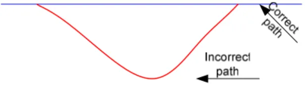
In this section, we find a method to derive an upper bound for the proposed STTC to demonstrate the novel scheme indeed can achieve diversity as we expected. For trellis codes, it is extremely complex to calculate the bit error rate (BER) and no efficient methods exist. Therefore we look for more accessible ways of obtaining a measure of performance. We consider the probability that a codeword error occurs. Such an error happens when the decoder follows a path in the trellis which diverges from the correct path somewhere in the trellis. The decoder will make an error if the path that follows through its trellis does not coincide with the path taken by the encoder. An error that follows a path in the trellis which diverges and emerges only once from the correct path in the trellis is called the first error
event shown in Fig3.1. In general, the error performance analysis of trellis codes is almost based on a code’s distance spectrum used in union bounding techniques. The distance spectrum for trellis codes is usually found by computer search. In [5], the authors derived design principles for space time channel codes over quasi-static fading channels. The design guidelines were based on maximizing the rank of the codeword difference matrix, in order to achieve the highest possible diversity over the quasi-static fading channel. In the following, we derive the performance bounds for proposed codes with some assumptions. Because the proposed STTC encoder is defined on complex field, it can be combined with multipath channel directly. Assuming that channel states information is known at receiver. We obtain the trellis diagram of the combined channels and from it we can get the minimum distance of the first error event assuming that all-zero path is transmitted. Furthermore we assume the error probability is dominated by the minimum distance, dmin. Because the distribution of channel random variable hj i, is complex Guassian distributed with zero mean and unit variance, its amplitude is Rayleigh distributed. Then we use the Rayleigh sum distributions and densities [7] to find the probability density function (PDF) of the random variable dmin. The upper bound for the proposed STTC can be calculated
from PDF of dmin. Although there is no closed form for the upper bound so far, the upper bound derived by our method is an evidence to explain that the proposed codes can achieve diversity orders as we expected. The method to derive the upper bound can simply be described as following steps:
1. Obtain dmin from the trellis of combined channels. 2. Find pdf of dminusing Rayleigh sum distribution. 3. Calculate upper bound for the proposed code.
1 2 1 2 1 1 2 2 t t t t c c c c− − − − 1 1 1 1 − − − − 1 1 1 1 1 2 1 2 1 1 t t t t c c c c− − 1 2/ t t t c c r 1 1 1 1 − − − − 1 1 1 1
Fig3.2 Trellis diagram for code1.3 with the combined channel
In the following, we take code 1.3 for example, two transmitted antenna and one receive antenna are used and channel length is two. From (2.28), the combined channel will be
(3.1) combined channels could be considered as tap delay line and the trellis diagram is shown in Fig3.2. We assume all-zero path is transmitted and define the Euclidean distance between two branches asdij = r ri− j 2 , where ri and rj are received signals of i-th and j-th
' 1 [ ,21 11 22, 12] h = h h +h h ' 2 [ 11, ( 12 21), 22] h = jh j h +h jh
Fig3.3 Minimum distance in the trellis diagram
branch respectively. From the trellis diagram in Fig3.3, we can obtain thedmin:
(3.2)
There are three terms in (3.2), each term presents an event error. We can easily see that the third term of (3.2) is always larger than the others, thus it does not need to be considered. (3.2) can be simplified as:
{
}
min min{ 11 12 21 22 , 21 11 22 12} min , d h h h h h h h h X Y = + + + + + + = (3.3)where is Rayleigh distributed .And let random variables X and Y be:
2 2 2 21 11 22 12 2jh + 2 (j h +h ) + 2jh h 2 2 2 11 21 12 21 11 22 22 12 , 2jh +2h + 2 (j h +h ) 2(+ h +h ) + 2jh +2h } 2 2 2 min min{ 2 11 2 ( 12 21) 2 22 , d = =l jh + j h +h + jh
X= h11 + h12 +h21 + h22
Y= h21 + h11+h22 + h12 , (3.4)
Figure 3.4 PDF of random varialve X
X ,Y are Rayleigh sum distributed ,and also they are independent and identical distribution (i.i.d) under this condition. Fig3.4 shows the pdf of the random variable X. For Rayleigh sum distribution, the approximated probability density function and cumulative density function (CDF) of N i.i.d. Rayleigh random variables are as following :
PDF: , x≥0 (3.5) where , (2N−1)!! (2= N−1)(2N−3)...3 1⋅ 1 2 [(2 1)!!]N b N N σ = − 2 2 1 2 1 ( ) 2 ( 1)! x N b N N x e f x b N − − − = −
CDF:
(3.6) .
Based on probability theorem, the probability density function of dmin can be calculated
as the form: 2 min 2 min 5 2 min min 2 3 0 ( ) 2 ( ) 2 ! k d b D k d d b f d e b k − = = ,dmin ≥ . (3.7) 0
Because the error probability is dominated by random variabledmin, we derive the upper
bound conditioned on channel as:
min 0 ( ) ( ) 2 s e E P X E H Q d N → ≤ (3.8)
where Es is the energy per symbol at each transmit antenna and Q function is the
complementary error function defined by
2 2 1 ( ) 2 t x Q x e dt π ∞ − = , (3.9) and we use the inequality
2 2 1 ( ) , 0 2 x Q x ≤ e− x≥ , (3.10)
in order to get an upper bound on the unconditional error probability, we need to average the channel with respect to the random variabledmin. The error probability can be upper
bounded by 2 2 1 2 0 ( ) 2 ( ) 1 ! k x N b k x b F x e k − − = = −
2 min 0 min 4 min min 0 1 ( ) ( ) 2 E d N e d D P ∞ e− f d d d = ≤ 2 2 min min 0 min 2 min 5 2 4 min min 2 3 0 0 ( ) 1 2 ( ) 2 2 ! k E d d N b d k d d b e e d d b k − − ∞ = = ≤ . (3.11)
Equation (3.11) is an upper bound for code 1.3.In the processing of proving the upper bound, some assumptions are needed to simplify calculation. Although the upper bound is not a tied bound, it provides an evidence to demonstrate that the proposed codes indeed can achieve diversity order we expected.
3.2 Space time turbo equalization
We use joint STTC/channel decoder based on MLSE to deal with ISI and exploit the multipath diversity gain. However, the computational complexity of the receiver is determined by the channel length and the number of trellis states. It grows exponentially when the channel length or the number of trellis states increase. Because of the high complexity, optimal receiver might be infeasible in most practical systems. For complexity reasons, the equalizer and decoder of most practical systems are separated. The straightforward way to implement this separate equalization and decoding process is for the equalizer to make hard decisions as to which sequence of channel symbols were transmitted and for these hard decisions to be mapped into their constituent binary code bits. The process of making hard decisions on the channel symbols actually destroys information pertaining to how likely each of the possible channel symbols might been, however. To mitigate the performance degradation made by hard decision, soft decision is considered. The ‘soft’ information can be converted into probabilities that each of the
received code bits takes on the value of zero or one that is precisely the form of information that can be exploited by a decoding algorithm. Many practical systems use this form of soft-input error control decoding by passing soft information between an equalizer and decoding algorithm. In order to approach the remarkable performance of optimal receivers with lower complexity, turbo equalization [14] is proposed. It is a receiver that the iterative process is between equalization and decoding. The transmitter and receiver structures for two transmit antennas are illustrated in Fig3.4. The BCJR algorithm [15] is used both in the equalizer and the decoder to estimate the soft information. At the center of the turbo equalizer are two BCJR algorithms that can operate on observations and prior information about individual bits or symbols. Only the extrinsic information is fed back in the iterative loop.
The MAP equalizer computers the LLR log-likelihood ratio of each group of information symbolsxt = . The soft output (i Λ xt = is given by [1][14] i)
{ | } ( ) log { 0 | } r t t r t P x i r x i P x r = Λ = = = / 0 / 1 ( ', ) 0 1 ( ', ) ( ') ( ', ) ( ) log ( ') ( ', ) ( ) i t t i t t t l l B t t t l l B l l l l l l l l α γ β α γ β − ∈ − ∈ = (3.12)
Where i denotes and information group from the set,{00,01,02,….., 2m− 21 m− },1 r is
the received sequence, i t
B is the set of transitions defined by St−1= → = , that are l' St l
caused by the input symbol i, where St is a trellis state at time t, and the probabilities
( )
t l
α , ( )βt l and ( 'γt l l, ) can be computed recursively. The symbol i with the largest
log-likelihood ratio in equation (3.12),i∈{00,01,02,….., 2m− 21 m− },is chosen as the 1
hard decision output.
The decoder operates on a trellis with Ms states. The forward recursive variables can be
computed as follows 1 1 '0 ( ) Ms ( ') ( 'i , ) t t t l l l l l α −α− γ = = ,l=0,1,2,....Ms− (3.13) 1 with the initial condition
αt(0) 1, ( ) 0,= αt l = l≠ 0
and the backward recursive variables can be computed as
1 1 1 '0 ( ) s ( ') ( , ') M i t t t l l l l l β − β+ γ + = = , l=0,1,2,....Ms − (3.14) 1 with the initial condition
βτ(0) 1, ( ) 0,= βτ l = l≠ . 0
The branch transition probability at time t, denoted by i ( ', )
t l l
, , 0 1 1 2 ( ) ( , ') exp( ), ( , ') (0) 2 0, R T n n L j n t j k n t k j n k i t i t t t r h x p i l l for l l B p othewise γ σ − = = = − = − ∈ (3.15) Where j t
r is the received signal by j-th antenna at time t, hj k n, , is k-th path of the channel
attenuation between n-th transmit antenna and j-th receive antenna , n t
x is the modulated symbol at time t, transmitted from n-th antenna and associated with the transition
1 '
t t
S− = → = , and l S l p it( )is the a priori probability of xt = . i
The iterative process between equalizer and decoder is that the soft information from equalizer is interleaved and taken into account in the decoding process and similarly the soft information from decoder is entered the equalizer, creating a feedback loop between equalizer and decoder. The performance of the BCJR algorithm can be greatly improved if good prior information is available. With iterative process, the performance of turbo equalizer would approach the optimal receiver.
3.3 Simulation results
In our simulation, a system with two transmit antennas and one receive antenna on the Rayleigh fading channel is used and 4-QAM modulation is used. We assume that the channel estimation is perfect.
Fig3.6 shows the comparison of STBC with Alamouti scheme, STTC and space time delay code (STDC) over flat fading channel. The system with two transmitted antennas and one received antenna and 4-QAM modulation is used. We assume that channel estimation is perfect. That is the channel state information is known at the receiver. We use the
conventional STTC with the coefficientsg1 =[(02),(20)],g2 =[(01),(10)] and the STDC
with one delay. Note that the STTC has better coding gain than STBC.
Fig3.7 shows the BER of codes 1.1, code 1.2 and code 1.3.The signals are transmitted over frequency selective channel with length of two. Note that code 1.3 has the highest diversity order. Two upper bounds for code1.1 and 1.3 calculated from our method are shown in Fig3.8 and Fig 3.9 respectively. In Fig3.10, simulation results shows that different upper bounds exactly have the diversity order of two, there and four.
Fig3.7 Bit error rate of code 1.1, 1.2 and 1.3
Fig3.9 Upper bound for code 1.3
Fig3.11 Performance of LCF-STTC and conventional STTC
over flat fading channel
Fig3.12 Performance of LCF-STTC with code 1.1 and conventional STTC over frequency selective channels.
Fig3.13 Performance of LCF-STTC with code 1.3 and conventional STTC over frequency selective channels.
Fig3.11 shows the performance comparison between LCF-STTC and conventional STTC over flat fading channel. In Fig3.11-Fig3.13, data1 is the code with coefficients g1=[(02),(20)] , g2 =[(01),(10)] ; data2 is the code with
coefficients g1 =[(02),(10)],g2 =[(22),(01)] ,and data3 is the code with coefficients 1 [(22),(10)], 2 [(02),(30)]
g = g = ;data4 and data5 are the same complex code. In Fig3.11 and Fig3.13, code1.3 is used, and code 1.1 is used in Fig3.12. Data5 is encoded with complex coefficients and decoded separately at the receiver whereas data4 is encoded with complex coefficients and jointly decoded at receiver. We see that Both two schemes have the same diversity order and the LCF-STTC has better performance than conventional STTC because the LCF-STTC has joint processing gain at the receiver. The performances of above two schemes over frequency selective channels are shown in Fig 3.12 and Fig3.13.The complex code satisfied designed criterion can combined with channel thus the receiver will extract mutipath diversity gain. With joint processing at receiver, the LCF-STTC has better performance than conventional STTC. Fig3.14 shows that with turbo equalizer, the performance of conventional STTC approaches the LCF-STTC after 0,1,2 and 5 iterations over frequency selective channels.
The complex-value coefficients of encoder can combine multipath channels directly and joint decoding based on MLSE receiver is used to exploit the multipath diversity gain. It shows that the proposed codes obtain the spatial diversity provided by multiple antennas and the temporal diversity provided by multipath. The conventional STTC designed for flat fading scenarios are guaranteed to extract spatial diversity at least if used in a frequency selective environment.
3.4 Summary
Space time trellis coding has been proposed as an effective approach to support high data rate transmission over fading channels. It is shown that the LCF-STTC with joint decoding based on MLSE receiver has better performance than the conventional STTC defined on finite ring over flat fading channel or frequency selective channels. Space time codes defined on complex field can combine multipath channels thus the receiver will extract the path diversity gain. Particular attention has been paid on the analytical performance evaluation of space-time coding. One method is to compute the code distance spectrum and apply the union bound technique to calculate the average pairwise error probability [16] [17]. A more accurate performance evaluation can be obtained with exact evaluation of pairwise error probability, rather than evaluating the bounds. This can be done by using residue methods based on the characteristic function technique [18]. Usually performance evaluation of STTC is analyzed over flat fading channels. However, performance analysis becomes more complicated and has more challenges over frequency selective channels. Our method proposed in previous section is analyzed under a simple and special case. Although the result is not a closed form, it provides an evidence to demonstrate that the proposed codes can achieve expected diversity order. The performance of the conventional STTC with turbo equalizer at the receiver will approach that of the LCF-STTC.
Chapter 4 Conclusion
It is shown that MLSE can be used together with space-time codes to exploit the multipath diversity gain. The focus is on the diversity benefit provided by the mutipath of ISI channels. For the case of STTC, a new complex-valued STTC is defined to facilitate the merge of the coding trellis and the channel effect, and thus a joint decoding based on MLSE can be realized. With this novel scheme, a full space and multipath diversity can be achieved besides a substantial coding gain. Space time code defined on complex field is discussed. The main advantage of space time codes defined on complex field is that their encoding arithmetic operation and the multipath channel arithmetic operations are all define on the complex field and therefore can be algebraically combined together. Then the receiver will extract multipath diversity gain. The LCF-STTC can be considered as one kind of delay code. Performance analysis of the LCF-STTC is presented. A method is found to derive an upper bound to show the novel scheme indeed achieve the diversity order as we expect.
Reference
[1] B. Vucetic and J. Yuan, “Space-time coding”, Wiley, Inc, 2003.
[2] A. Paulraj, R. Nabar, and D. Gore, “Introduction to Space-Time Wireless Communications”, 1th ed. United Kingdom at the University Press, Cambridge 2003.
[3] N. Seshadri and J. H. Winters, “Two signaling schemes for improving the error performance of FDD transmission systems using transmitter antenna diversity”, in
Proc. 1993 IEEE Vehicular Technology Conf. (VTC 43rd), May 1993, pp. 508-511.
[4] S. M. Alamouti, “A simple transmit diversity technique for wireless communication”,
IEEE J. Sel. Areas Comm., 16(8), 1451-1458, Oct. 1998.
[5] V. Tarokh, N. Seshdri and A. R. Calderbank, “Space-Time Codes for High Data Rate Wireless Communication: Performance Analysis and Code Construction“, IEEE
Trans. Inform. Theory, vol.44, no. 2, pp.744-765, Mar. 1998.
[6] A.Wong, J. Yuan, J. Choi, S. R.Kim, I-K Choi, and D-S Kwon,” Design of 16-QAM space time trellis codes for quasi-static fading channels. ” IEEE Vehicular Technology Conference, pp. 880-883, Malin, Italy,Oct. 2004.
[7] Jeremiah Hu and Norman C.Beaulieu ,”Accurate simple closed-form approximations to Rayleigh sum distributions and densities”. IEEE communications letters, vol.9, NO. 2, Feb 2005.
[8] J. H. Winters, “Switched diversity with feedback for DPSK mobile radio systems”,
IEEE Trans. Vehicular Technology, vol. 32, pp. 134-150, 1983.
[9] J. H. Winters, “The diversity gain of transmit diversity in wireless systems with Rayleigh fading”, in Proc. 1994 ICC/SUPERCOMM, New Orleans, LA, May 1994, vol. 2, pp. 1121-1125.