利用Isomap學習及VLMM技術來分析人類之動作

國立交通大學

資訊工程學系

博士論文

利用

Isomap 學習及 VLMM 技術來分析人類之動作

A Study on Video-Based Human Action Analysis by Isomap

Learning and VLMM Techniques

研 究 生： 梁祐銘

指導教授： 廖弘源 教授

林正中 教授

A Study on Video-Based Human Action Analysis by Isomap Learning and

VLMM Techniques

研 究 生：梁祐銘 Student：Yu-Ming Liang

指導教授：廖弘源 Advisor：Hong-Yuan Mark Liao

林正中

Cheng-Chung

Lin

國 立 交 通 大 學

資 訊 工 程 學 系

博 士 論 文

A Dissertation

Submitted to Department of Computer Science College of Computer Science

National Chiao Tung University in Partial Fulfillment of the Requirements

for the Degree of Doctor of Philosophy

in

Computer Science January 2009

利用

Isomap 學習及 VLMM 技術來分析人類之動作

學生：梁祐銘

指導教授：廖弘源 博士

林正中 博士

國立交通大學資訊工程學系(研究所)博士班

摘

要

人類動作分析是一個很基本的研究議題，並且被廣泛地應用在許多不同 的研究領域。本論文提出了兩種適於人類動作分析之相關應用的視訊處理技 衛。首先，為了自動化分析一段冗長且尚未被切割過之人類動作視訊資料， 我 們 提 出 一 個 以 流 形 學 習(manifold learning) 技 術 為 基 礎 之 非 監 督 式 (unsupervised)人類動作分析架構。為了有效地分析人類動作，非監督式學習 的方法比監督式學習的方法更為適合，主要是因為非監督式學習的方法事先 不需要太多的人為介入。然而，複雜的人類動作使得非監式學習的方法更具 挑戰性。在這項研究中，我們首先從一個訓練用的動作序列中取得一個成對 的人類姿勢距離矩陣。接著再利用等構映圖(Isomap)演算法從此矩陣中建構 出低維度的結構。因此，訓練用的動作序列可以被映射到等構映圖空間中的 流形軌跡(manifold trajectory)。為了有效地找出連續兩個單元(atomic)動作軌 跡中的中斷點，我們將等構映圖空間中的流形軌跡描述為低維度的時間序 i

列。我們接著再利用時間分割的技術將此時間序列分割成許多次級序列，每 個次級序列都代表一個單元動作。然後，我們利用動態時間校正(dynamic time warping)的技術來對這些單元動作序列分群。最後，我們依據分群結果來學 習單元動作，並且再利用最近鄰算法(nearest neighbor rule)對單元動作做分 類。假如介於輸入的動作序列與最相近的群平均單元動作序列的距離大於某 個門檻值時，我們便將此輸入的動作序列視為未知的單元動作。

在 第 二 項 研 究 中 ， 我 們 提 出 了 一 個 利 用 可 變 長 度 馬 可 夫 模 型 (variable-length Markov models)技術來學習及辨認單元人類動作的架構。本架 再包含兩個主要模組：姿勢標記模組及可變長度馬可夫模型之單元動作學習 及辨認模組。首先，我們修改外形上下文(shape context)的技術來發展一個姿 勢樣板(posture template)選擇的演算法。被選取的姿勢樣板可形成一個碼本 (codebook)，利用此碼本我們可以將輸入的姿勢序列轉變為離散的符號序列。 接著，我們利用可變長度馬可夫模型技術來學習對應於訓練用的單元動作之 符號序列。最後，我們可將被建構的可變長度馬可夫模型轉換成隱藏式馬可 夫模型(HMM)，並且再利用它來辨認輸入的單元動作。這項研究主要是結合 可變長度馬可夫模型在學習方面的傑出好處及隱藏式馬可夫模型在容錯辨識 能力的好處。

A Study on Video-Based Human Action Analysis

by Isomap Learning and VLMM Techniques

Student：Yu-Ming Liang Advisors：Dr. Hong-Yuan Mark Liao

Dr. Cheng-Chung Lin

Department of Computer Science

National Chiao Tung University

Abstract

Human Action Analysis is a fundamental issue that can be applied to different application domains. In this dissertation, we propose two video processing techniques for human action analysis. First, to automatically analyze a long and unsegmented human action video sequence, we propose a framework for unsupervised analysis of human action based on manifold learning. To analyze of human action, unsupervised learning is superior to supervised one because the former does not require much human intervention beforehand. However, the complex nature of human action analysis makes unsupervised learning a challenging task. In this work, a pairwise human posture distance matrix is derived from a training action sequence. Then, the isometric feature mapping (Isomap) algorithm is applied to construct a low-dimensional structure from the distance matrix. Consequently, the training action sequence is mapped

into a manifold trajectory in the Isomap space. To identify the break points between any two successive atomic action trajectories, we represent the manifold trajectory in the Isomap space as a time series of low-dimensional points. A temporal segmentation technique is then applied to segment the time series into sub-series, each of which corresponds to an atomic action. Next, the dynamic time warping (DTW) approach is used to cluster atomic action sequences. Finally, we use the clustering results to learn and classify atomic actions according to the nearest neighbor rule. If the distance between the input sequence and the nearest mean sequence is greater than a threshold, it is regarded as an unknown atomic action.

In our second work, we propose a framework for learning and recognizing atomic human actions using variable-length Markov models (VLMMs). The framework comprises two modules: a posture labeling module, and a VLMM atomic action learning and recognition module. In the first stage, a posture template selection algorithm is developed based on a modified shape context matching technique. The selected posture templates form a codebook which can be used to convert input posture sequences into discrete symbol sequences for subsequent processing. Then, the VLMM technique is applied to learn the training symbol sequences of atomic actions. Finally, the constructed VLMMs are transformed into hidden Markov models (HMMs) for recognizing input atomic actions. This approach combines the advantages of the excellent learning function of a VLMM and the fault-tolerant recognition ability of an HMM.

誌謝

二十幾年來的求學過程，終於隨著本論文的完成而告結束。在博士求學 期間，對我而言，是影響我人生最大的一段歷程。在這段過程中，遭遇了一 些人生的大事，很慶幸有良師、益友陪我走過，讓我能堅持地走完這段漫長 的求學過程。 首先，要感謝中研院資訊所的指導教授廖弘源老師，在我大四時帶領我 進入這個領域，並且從碩士一路指導到現在完成博士學位。在這段日子裏， 他不但教導我許多作研究的態度與方法，也教導了我許多做人做事的原則， 並且給予我許多生活上的協助，真的很有福氣能當他的學生。其次，要感謝 中研院資訊所施純傑老師，不管我在研究上或生活上遇到困難時，都可以提 供我許多寶貴的建議與思考的方向，讓我獲益良多。另外，要感謝暨南大學 資工系石勝文老師，在這段研究過程中，給了我許多研究上的建議，並且教 導我論文寫作的技巧。此外，也要感謝校內的指導教授林正中老師，在博士 求學過程中，給予我許多校內事務上的協助。因為有了這些老師的付出，這 篇論文才得以在此呈現。 感謝佛光大學副校長范國清教授、台科大電子系方文賢教授、本系蔡文 祥教授與莊仁輝教授，在百忙之中仍撥空指導並審查論文，實在惠我良多。 同時也要感謝中研究資訊所多媒體技術實驗室的伙伴們：陳敦裕博士、蘇志 文博士、林學億博士、曾易聰博士、孫士韋博士、張俊雄博士、賴育駿、羅 v

使得研究的旅程不孤單。

最後，也是最重要的，要感謝我最親愛的家人，他們總是給予我最大的 關心與支持，讓我能夠全心全力投入研究中，才造就了今日的我。

一聲聲的感謝，仍道不出我感恩之心，說不盡我感激之情，謹於此，獻 上我最大的祝福，願大家都幸福美滿。

Table of Contents

Abstract in Chinese i

Abstract in English iii

Acknowledgements in Chinese v

Table of Contents vii

List of Tables x

List of Figures xi

1. Introduction 1

1.1 Motivation ⋅⋅⋅⋅⋅⋅⋅⋅⋅⋅⋅⋅⋅⋅⋅⋅⋅⋅⋅⋅⋅⋅⋅⋅⋅⋅⋅⋅⋅⋅⋅⋅⋅⋅⋅⋅⋅⋅⋅⋅⋅⋅⋅⋅⋅⋅⋅⋅⋅⋅⋅⋅⋅⋅⋅⋅⋅⋅⋅⋅⋅⋅⋅⋅⋅⋅⋅⋅⋅⋅⋅⋅⋅⋅⋅⋅⋅⋅⋅⋅⋅⋅⋅⋅ 1 1.2 Related Work ⋅⋅⋅⋅⋅⋅⋅⋅⋅⋅⋅⋅⋅⋅⋅⋅⋅⋅⋅⋅⋅⋅⋅⋅⋅⋅⋅⋅⋅⋅⋅⋅⋅⋅⋅⋅⋅⋅⋅⋅⋅⋅⋅⋅⋅⋅⋅⋅⋅⋅⋅⋅⋅⋅⋅⋅⋅⋅⋅⋅⋅⋅⋅⋅⋅⋅⋅⋅⋅⋅⋅⋅⋅⋅⋅⋅⋅⋅⋅⋅ 2 1.2.1 Survey on Atomic Action Segmentation ⋅⋅⋅⋅⋅⋅⋅⋅⋅⋅⋅⋅⋅⋅⋅⋅⋅⋅⋅⋅⋅⋅⋅⋅⋅⋅ 2 1.2.2 Survey on Atomic Action Recognition ⋅⋅⋅⋅⋅⋅⋅⋅⋅⋅⋅⋅⋅⋅⋅⋅⋅⋅⋅⋅⋅⋅⋅⋅⋅⋅⋅⋅ 4 1.3 Overview of the Proposed Methods ⋅⋅⋅⋅⋅⋅⋅⋅⋅⋅⋅⋅⋅⋅⋅⋅⋅⋅⋅⋅⋅⋅⋅⋅⋅⋅⋅⋅⋅⋅⋅⋅⋅⋅⋅⋅⋅⋅⋅⋅⋅⋅⋅⋅⋅ 9 1.4 Dissertation Organization ⋅⋅⋅⋅⋅⋅⋅⋅⋅⋅⋅⋅⋅⋅⋅⋅⋅⋅⋅⋅⋅⋅⋅⋅⋅⋅⋅⋅⋅⋅⋅⋅⋅⋅⋅⋅⋅⋅⋅⋅⋅⋅⋅⋅⋅⋅⋅⋅⋅⋅⋅⋅⋅⋅⋅⋅⋅⋅⋅⋅⋅ 11

and Variable-Length Markov Model 13

2.1 Shape Context ⋅⋅⋅⋅⋅⋅⋅⋅⋅⋅⋅⋅⋅⋅⋅⋅⋅⋅⋅⋅⋅⋅⋅⋅⋅⋅⋅⋅⋅⋅⋅⋅⋅⋅⋅⋅⋅⋅⋅⋅⋅⋅⋅⋅⋅⋅⋅⋅⋅⋅⋅⋅⋅⋅⋅⋅⋅⋅⋅⋅⋅⋅⋅⋅⋅⋅⋅⋅⋅⋅⋅⋅⋅⋅⋅⋅⋅⋅ 13 2.2 Manifold Learning ⋅⋅⋅⋅⋅⋅⋅⋅⋅⋅⋅⋅⋅⋅⋅⋅⋅⋅⋅⋅⋅⋅⋅⋅⋅⋅⋅⋅⋅⋅⋅⋅⋅⋅⋅⋅⋅⋅⋅⋅⋅⋅⋅⋅⋅⋅⋅⋅⋅⋅⋅⋅⋅⋅⋅⋅⋅⋅⋅⋅⋅⋅⋅⋅⋅⋅⋅⋅⋅⋅⋅ 16 2.2.1 Isomap Algorithm ⋅⋅⋅⋅⋅⋅⋅⋅⋅⋅⋅⋅⋅⋅⋅⋅⋅⋅⋅⋅⋅⋅⋅⋅⋅⋅⋅⋅⋅⋅⋅⋅⋅⋅⋅⋅⋅⋅⋅⋅⋅⋅⋅⋅⋅⋅⋅⋅⋅⋅⋅⋅⋅⋅⋅⋅⋅⋅⋅⋅⋅⋅⋅ 19 2.3 Variable-Length Markov Model ⋅⋅⋅⋅⋅⋅⋅⋅⋅⋅⋅⋅⋅⋅⋅⋅⋅⋅⋅⋅⋅⋅⋅⋅⋅⋅⋅⋅⋅⋅⋅⋅⋅⋅⋅⋅⋅⋅⋅⋅⋅⋅⋅⋅⋅⋅⋅⋅⋅⋅⋅ 22 2.3.1 VLMM Learning ⋅⋅⋅⋅⋅⋅⋅⋅⋅⋅⋅⋅⋅⋅⋅⋅⋅⋅⋅⋅⋅⋅⋅⋅⋅⋅⋅⋅⋅⋅⋅⋅⋅⋅⋅⋅⋅⋅⋅⋅⋅⋅⋅⋅⋅⋅⋅⋅⋅⋅⋅⋅⋅⋅⋅⋅⋅⋅⋅⋅⋅⋅⋅⋅⋅ 24 2.3.2 VLMM Recognition ⋅⋅⋅⋅⋅⋅⋅⋅⋅⋅⋅⋅⋅⋅⋅⋅⋅⋅⋅⋅⋅⋅⋅⋅⋅⋅⋅⋅⋅⋅⋅⋅⋅⋅⋅⋅⋅⋅⋅⋅⋅⋅⋅⋅⋅⋅⋅⋅⋅⋅⋅⋅⋅⋅⋅⋅⋅⋅⋅⋅ 27

3. Unsupervised Analysis of Human Action Based on Manifold

Learning 29

3.1 Introduction ⋅⋅⋅⋅⋅⋅⋅⋅⋅⋅⋅⋅⋅⋅⋅⋅⋅⋅⋅⋅⋅⋅⋅⋅⋅⋅⋅⋅⋅⋅⋅⋅⋅⋅⋅⋅⋅⋅⋅⋅⋅⋅⋅⋅⋅⋅⋅⋅⋅⋅⋅⋅⋅⋅⋅⋅⋅⋅⋅⋅⋅⋅⋅⋅⋅⋅⋅⋅⋅⋅⋅⋅⋅⋅⋅⋅⋅⋅⋅⋅⋅⋅ 29 3.2 The Proposed Approach ⋅⋅⋅⋅⋅⋅⋅⋅⋅⋅⋅⋅⋅⋅⋅⋅⋅⋅⋅⋅⋅⋅⋅⋅⋅⋅⋅⋅⋅⋅⋅⋅⋅⋅⋅⋅⋅⋅⋅⋅⋅⋅⋅⋅⋅⋅⋅⋅⋅⋅⋅⋅⋅⋅⋅⋅⋅⋅⋅⋅⋅⋅⋅ 32 3.2.1 Posture Representation and Matching ⋅⋅⋅⋅⋅⋅⋅⋅⋅⋅⋅⋅⋅⋅⋅⋅⋅⋅⋅⋅⋅⋅⋅⋅⋅⋅⋅⋅⋅⋅⋅⋅⋅ 33 3.2.2 Isomap Learning of Human Action ⋅⋅⋅⋅⋅⋅⋅⋅⋅⋅⋅⋅⋅⋅⋅⋅⋅⋅⋅⋅⋅⋅⋅⋅⋅⋅⋅⋅⋅⋅⋅⋅⋅ 37 3.2.3 Temporal Segmentation ⋅⋅⋅⋅⋅⋅⋅⋅⋅⋅⋅⋅⋅⋅⋅⋅⋅⋅⋅⋅⋅⋅⋅⋅⋅⋅⋅⋅⋅⋅⋅⋅⋅⋅⋅⋅⋅⋅⋅⋅⋅⋅⋅⋅⋅⋅⋅⋅⋅⋅⋅⋅⋅⋅⋅ 38 3.2.4 Atomic Action Clustering ⋅⋅⋅⋅⋅⋅⋅⋅⋅⋅⋅⋅⋅⋅⋅⋅⋅⋅⋅⋅⋅⋅⋅⋅⋅⋅⋅⋅⋅⋅⋅⋅⋅⋅⋅⋅⋅⋅⋅⋅⋅⋅⋅⋅⋅⋅⋅⋅⋅⋅⋅⋅ 40 3.2.5 Atomic Action Learning and Classification ⋅⋅⋅⋅⋅⋅⋅⋅⋅⋅⋅⋅⋅⋅⋅⋅⋅⋅⋅⋅⋅⋅⋅⋅ 41 3.3 Experiments ⋅⋅⋅⋅⋅⋅⋅⋅⋅⋅⋅⋅⋅⋅⋅⋅⋅⋅⋅⋅⋅⋅⋅⋅⋅⋅⋅⋅⋅⋅⋅⋅⋅⋅⋅⋅⋅⋅⋅⋅⋅⋅⋅⋅⋅⋅⋅⋅⋅⋅⋅⋅⋅⋅⋅⋅⋅⋅⋅⋅⋅⋅⋅⋅⋅⋅⋅⋅⋅⋅⋅⋅⋅⋅⋅⋅⋅⋅⋅⋅⋅ 45 3.4 Concluding Remarks ⋅⋅⋅⋅⋅⋅⋅⋅⋅⋅⋅⋅⋅⋅⋅⋅⋅⋅⋅⋅⋅⋅⋅⋅⋅⋅⋅⋅⋅⋅⋅⋅⋅⋅⋅⋅⋅⋅⋅⋅⋅⋅⋅⋅⋅⋅⋅⋅⋅⋅⋅⋅⋅⋅⋅⋅⋅⋅⋅⋅⋅⋅⋅⋅⋅⋅⋅⋅ 54

4. Learning Atomic Human Actions Using Variable-Length

Markov Models 57

4.1 Introduction ⋅⋅⋅⋅⋅⋅⋅⋅⋅⋅⋅⋅⋅⋅⋅⋅⋅⋅⋅⋅⋅⋅⋅⋅⋅⋅⋅⋅⋅⋅⋅⋅⋅⋅⋅⋅⋅⋅⋅⋅⋅⋅⋅⋅⋅⋅⋅⋅⋅⋅⋅⋅⋅⋅⋅⋅⋅⋅⋅⋅⋅⋅⋅⋅⋅⋅⋅⋅⋅⋅⋅⋅⋅⋅⋅⋅⋅⋅⋅⋅⋅⋅ 57 4.2 The Proposed Method for Atomic Action Recognition ⋅⋅⋅⋅⋅⋅⋅⋅⋅⋅⋅⋅⋅⋅⋅⋅ 60 4.2.1 Posture Labeling ⋅⋅⋅⋅⋅⋅⋅⋅⋅⋅⋅⋅⋅⋅⋅⋅⋅⋅⋅⋅⋅⋅⋅⋅⋅⋅⋅⋅⋅⋅⋅⋅⋅⋅⋅⋅⋅⋅⋅⋅⋅⋅⋅⋅⋅⋅⋅⋅⋅⋅⋅⋅⋅⋅⋅⋅⋅⋅⋅⋅⋅⋅⋅⋅⋅ 61 4.2.2 Human Action Sequence Learning and Recognition ⋅⋅⋅⋅⋅⋅⋅⋅⋅⋅ 64 4.3 Experiments ⋅⋅⋅⋅⋅⋅⋅⋅⋅⋅⋅⋅⋅⋅⋅⋅⋅⋅⋅⋅⋅⋅⋅⋅⋅⋅⋅⋅⋅⋅⋅⋅⋅⋅⋅⋅⋅⋅⋅⋅⋅⋅⋅⋅⋅⋅⋅⋅⋅⋅⋅⋅⋅⋅⋅⋅⋅⋅⋅⋅⋅⋅⋅⋅⋅⋅⋅⋅⋅⋅⋅⋅⋅⋅⋅⋅⋅⋅⋅⋅⋅ 69 4.4 Concluding Remarks ⋅⋅⋅⋅⋅⋅⋅⋅⋅⋅⋅⋅⋅⋅⋅⋅⋅⋅⋅⋅⋅⋅⋅⋅⋅⋅⋅⋅⋅⋅⋅⋅⋅⋅⋅⋅⋅⋅⋅⋅⋅⋅⋅⋅⋅⋅⋅⋅⋅⋅⋅⋅⋅⋅⋅⋅⋅⋅⋅⋅⋅⋅⋅⋅⋅⋅⋅⋅ 81

5. Conclusions and Future Work 83

5.1 Conclusions ⋅⋅⋅⋅⋅⋅⋅⋅⋅⋅⋅⋅⋅⋅⋅⋅⋅⋅⋅⋅⋅⋅⋅⋅⋅⋅⋅⋅⋅⋅⋅⋅⋅⋅⋅⋅⋅⋅⋅⋅⋅⋅⋅⋅⋅⋅⋅⋅⋅⋅⋅⋅⋅⋅⋅⋅⋅⋅⋅⋅⋅⋅⋅⋅⋅⋅⋅⋅⋅⋅⋅⋅⋅⋅⋅⋅⋅⋅⋅⋅⋅⋅ 83 5.2 Future work ⋅⋅⋅⋅⋅⋅⋅⋅⋅⋅⋅⋅⋅⋅⋅⋅⋅⋅⋅⋅⋅⋅⋅⋅⋅⋅⋅⋅⋅⋅⋅⋅⋅⋅⋅⋅⋅⋅⋅⋅⋅⋅⋅⋅⋅⋅⋅⋅⋅⋅⋅⋅⋅⋅⋅⋅⋅⋅⋅⋅⋅⋅⋅⋅⋅⋅⋅⋅⋅⋅⋅⋅⋅⋅⋅⋅⋅⋅⋅⋅⋅⋅ 85

Bibliography 87

Publication List 99

List of Tables

4.1. The results of atomic action recognition using the training data 73 4.2. Comparison of our method’s recognition rate with that of the

HMM computed with the test data obtained from nine different human subjects ⋅⋅⋅⋅⋅⋅⋅⋅⋅⋅⋅⋅⋅⋅⋅⋅⋅⋅⋅⋅⋅⋅⋅⋅⋅⋅⋅⋅⋅⋅⋅⋅⋅⋅⋅⋅⋅⋅⋅⋅⋅⋅⋅⋅⋅⋅⋅⋅⋅⋅⋅⋅⋅⋅⋅⋅⋅⋅⋅⋅⋅⋅⋅⋅⋅⋅⋅⋅⋅⋅⋅⋅⋅⋅⋅ 77 4.3. Comparison of our method’s recognition rate with that of the

AME plus NN method and the MMS plus NN method for the public database ⋅⋅⋅⋅⋅⋅⋅⋅⋅⋅⋅⋅⋅⋅⋅⋅⋅⋅⋅⋅⋅⋅⋅⋅⋅⋅⋅⋅⋅⋅⋅⋅⋅⋅⋅⋅⋅⋅⋅⋅⋅⋅⋅⋅⋅⋅⋅⋅⋅⋅⋅⋅⋅⋅⋅⋅⋅⋅⋅⋅⋅⋅⋅⋅⋅⋅⋅⋅⋅⋅⋅⋅⋅⋅⋅ 80

List of Figures

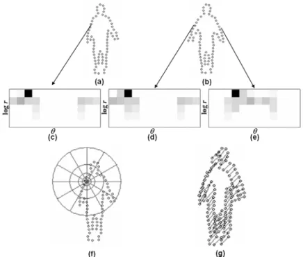
2.1. Shape context computation and matching: (a) and (b) show the sampled points of two shapes; and (c)-(e) are the local shape contexts corresponding to different reference points. A diagram of the log-polar space is shown in (f), while (g) shows the correspondence between points computed using a bipartite graph matching method. ⋅⋅⋅⋅⋅⋅⋅⋅⋅⋅⋅⋅⋅⋅⋅⋅⋅⋅⋅⋅⋅⋅⋅⋅⋅⋅⋅⋅⋅⋅⋅⋅⋅⋅⋅⋅⋅⋅⋅⋅⋅⋅⋅⋅⋅⋅⋅⋅⋅⋅⋅⋅⋅⋅⋅⋅⋅⋅⋅⋅⋅ 14 2.2. The 2-dimensional embedding manifolds of “Swiss Roll”

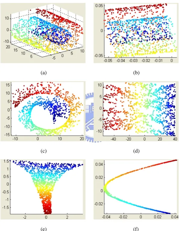
computed with five different dimensionality reduction techniques: (a) Original 3-D data set, (b) PCA, (c) MDS, (d) Isomap, (e) LLE, and (f) LE. ⋅⋅⋅⋅⋅⋅⋅⋅⋅⋅⋅⋅⋅⋅⋅⋅⋅⋅⋅⋅⋅⋅⋅⋅⋅⋅⋅⋅⋅⋅⋅⋅⋅⋅⋅⋅⋅⋅⋅⋅⋅⋅⋅⋅⋅⋅⋅⋅⋅⋅⋅⋅⋅ 18 2.3. An example of a VLMM ⋅⋅⋅⋅⋅⋅⋅⋅⋅⋅⋅⋅⋅⋅⋅⋅⋅⋅⋅⋅⋅⋅⋅⋅⋅⋅⋅⋅⋅⋅⋅⋅⋅⋅⋅⋅⋅⋅⋅⋅⋅⋅⋅⋅⋅⋅⋅⋅⋅⋅⋅⋅⋅⋅⋅⋅⋅⋅⋅⋅⋅ 23 2.4. The PST for constructing the VLMM shown in Figure 2.3 ⋅⋅⋅⋅⋅⋅⋅⋅ 24 3.1. The flowchart of the proposed method ⋅⋅⋅⋅⋅⋅⋅⋅⋅⋅⋅⋅⋅⋅⋅⋅⋅⋅⋅⋅⋅⋅⋅⋅⋅⋅⋅⋅⋅⋅⋅⋅⋅⋅⋅⋅⋅⋅⋅ 33 3.2. Human action consists of a series of discrete human postures 34 3.3. Convex hull-shape contexts matching: (a) and (b) show the

convex hull vertices of two shapes; (c) shows the correspondence between the convex hull vertices determined using shape matching. ⋅⋅⋅⋅⋅⋅⋅⋅⋅⋅⋅⋅⋅⋅⋅⋅⋅⋅⋅⋅⋅⋅⋅⋅⋅⋅⋅⋅⋅⋅⋅⋅⋅⋅⋅⋅⋅⋅⋅⋅⋅⋅⋅⋅⋅⋅⋅⋅⋅⋅⋅⋅⋅⋅⋅⋅⋅⋅⋅⋅⋅⋅⋅⋅ 36 3.4. The residual variance of Isomap on the training data ⋅⋅⋅⋅⋅⋅⋅⋅⋅⋅⋅⋅⋅⋅⋅⋅⋅ 37

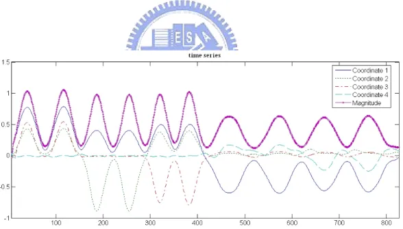
the action sequence projected on to (a) the first three dimensions (dims. 1-3), and (b) the last three dimensions (dims. 2-4). ⋅⋅⋅⋅⋅⋅⋅⋅⋅⋅⋅⋅⋅⋅⋅⋅⋅⋅⋅⋅⋅⋅⋅⋅⋅⋅⋅⋅⋅⋅⋅⋅⋅⋅⋅⋅⋅⋅⋅⋅⋅⋅⋅⋅⋅⋅⋅⋅⋅⋅⋅⋅⋅⋅⋅⋅⋅⋅⋅⋅⋅⋅⋅⋅⋅⋅⋅⋅⋅⋅⋅⋅⋅⋅⋅⋅⋅⋅⋅⋅⋅ 38 3.6. The time series of data points and corresponding magnitudes

after Gaussian smoothing ⋅⋅⋅⋅⋅⋅⋅⋅⋅⋅⋅⋅⋅⋅⋅⋅⋅⋅⋅⋅⋅⋅⋅⋅⋅⋅⋅⋅⋅⋅⋅⋅⋅⋅⋅⋅⋅⋅⋅⋅⋅⋅⋅⋅⋅⋅⋅⋅⋅⋅⋅⋅⋅⋅⋅⋅⋅⋅⋅ 39 3.7. The five classes of atomic actions used for training ⋅⋅⋅⋅⋅⋅⋅⋅⋅⋅⋅⋅⋅⋅⋅⋅⋅⋅⋅ 46 3.8. The Isomap space constructed from the training data: the 4-D

manifold trajectory projected on to (a) the first three dimensions (dims. 1-3), and (b) the last three dimensions (dims. 2-4). ⋅⋅⋅⋅⋅⋅⋅⋅⋅⋅⋅⋅⋅⋅⋅⋅⋅⋅⋅⋅⋅⋅⋅⋅⋅⋅⋅⋅⋅⋅⋅⋅⋅⋅⋅⋅⋅⋅⋅⋅⋅⋅⋅⋅⋅⋅⋅⋅⋅⋅⋅⋅⋅⋅⋅⋅⋅⋅⋅⋅⋅⋅⋅⋅⋅⋅⋅⋅⋅⋅⋅⋅⋅⋅⋅⋅⋅⋅⋅⋅⋅ 46 3.9. The results of temporal segmentation of (a) the time series, and

(b) the human posture sequence. ⋅⋅⋅⋅⋅⋅⋅⋅⋅⋅⋅⋅⋅⋅⋅⋅⋅⋅⋅⋅⋅⋅⋅⋅⋅⋅⋅⋅⋅⋅⋅⋅⋅⋅⋅⋅⋅⋅⋅⋅⋅⋅⋅⋅⋅⋅⋅⋅ 47 3.10. Five mean trajectories representing the five classes of atomic

actions are plotted in different colors. ⋅⋅⋅⋅⋅⋅⋅⋅⋅⋅⋅⋅⋅⋅⋅⋅⋅⋅⋅⋅⋅⋅⋅⋅⋅⋅⋅⋅⋅⋅⋅⋅⋅⋅⋅⋅⋅⋅⋅⋅ 47 3.11. The atomic action trajectories constructed from test data

sequence 1 and the classification results ⋅⋅⋅⋅⋅⋅⋅⋅⋅⋅⋅⋅⋅⋅⋅⋅⋅⋅⋅⋅⋅⋅⋅⋅⋅⋅⋅⋅⋅⋅⋅⋅⋅⋅⋅⋅ 49 3.12. The atomic action trajectories constructed from test data

sequence 2 and the classification results ⋅⋅⋅⋅⋅⋅⋅⋅⋅⋅⋅⋅⋅⋅⋅⋅⋅⋅⋅⋅⋅⋅⋅⋅⋅⋅⋅⋅⋅⋅⋅⋅⋅⋅⋅⋅ 49 3.13. The atomic action trajectories constructed from test data

sequence 3 superimposed on to the five learned exemplar trajectories. ⋅⋅⋅⋅⋅⋅⋅⋅⋅⋅⋅⋅⋅⋅⋅⋅⋅⋅⋅⋅⋅⋅⋅⋅⋅⋅⋅⋅⋅⋅⋅⋅⋅⋅⋅⋅⋅⋅⋅⋅⋅⋅⋅⋅⋅⋅⋅⋅⋅⋅⋅⋅⋅⋅⋅⋅⋅⋅⋅⋅⋅⋅⋅⋅⋅⋅⋅⋅⋅⋅⋅⋅⋅⋅⋅⋅⋅⋅⋅⋅⋅ 50

3.14. The selected key data points and the reconstructed Isomap space ⋅⋅⋅⋅⋅⋅⋅⋅⋅⋅⋅⋅⋅⋅⋅⋅⋅⋅⋅⋅⋅⋅⋅⋅⋅⋅⋅⋅⋅⋅⋅⋅⋅⋅⋅⋅⋅⋅⋅⋅⋅⋅⋅⋅⋅⋅⋅⋅⋅⋅⋅⋅⋅⋅⋅⋅⋅⋅⋅⋅⋅⋅⋅⋅⋅⋅⋅⋅⋅⋅⋅⋅⋅⋅⋅⋅⋅⋅⋅⋅⋅⋅⋅⋅⋅⋅⋅⋅⋅⋅⋅ 52 3.15. The average distance between the original Isomap and the

reconstructed Isomap using different percentages of selected key points over the total number of data points ⋅⋅⋅⋅⋅⋅⋅⋅⋅⋅⋅⋅⋅⋅⋅⋅⋅⋅⋅⋅⋅⋅⋅⋅⋅ 52 3.16. The reconstructed atomic action trajectories derived from test

data sequence 1 and the classification results based on the simplified action classification approach. ⋅⋅⋅⋅⋅⋅⋅⋅⋅⋅⋅⋅⋅⋅⋅⋅⋅⋅⋅⋅⋅⋅⋅⋅⋅⋅⋅⋅⋅⋅⋅⋅⋅⋅ 53 3.17. The reconstructed atomic action trajectories derived from test

data sequence 2 and the classification results based on the simplified action classification approach. ⋅⋅⋅⋅⋅⋅⋅⋅⋅⋅⋅⋅⋅⋅⋅⋅⋅⋅⋅⋅⋅⋅⋅⋅⋅⋅⋅⋅⋅⋅⋅⋅⋅⋅ 53 3.18. The reconstructed atomic action trajectories derived from test

data sequence 3 based on the simplified action classification approach superimposed on to the five learned exemplar trajectories. ⋅⋅⋅⋅⋅⋅⋅⋅⋅⋅⋅⋅⋅⋅⋅⋅⋅⋅⋅⋅⋅⋅⋅⋅⋅⋅⋅⋅⋅⋅⋅⋅⋅⋅⋅⋅⋅⋅⋅⋅⋅⋅⋅⋅⋅⋅⋅⋅⋅⋅⋅⋅⋅⋅⋅⋅⋅⋅⋅⋅⋅⋅⋅⋅⋅⋅⋅⋅⋅⋅⋅⋅⋅⋅⋅⋅⋅⋅⋅⋅⋅ 54 4.1. Block diagram of the proposed posture labeling process ⋅⋅⋅⋅⋅⋅⋅⋅⋅⋅⋅⋅ 62 4.2. (a) The VLMM constructed with the original input training

sequence; (b) the original VLMM constructed with the preprocessed training sequence; (c) the modified VLMM, which includes the possibility of self-transition. ⋅⋅⋅⋅⋅⋅⋅⋅⋅⋅⋅⋅⋅⋅⋅⋅⋅⋅⋅⋅⋅⋅⋅ 67 4.3. The distribution of observation error, obtained using the

training data. ⋅⋅⋅⋅⋅⋅⋅⋅⋅⋅⋅⋅⋅⋅⋅⋅⋅⋅⋅⋅⋅⋅⋅⋅⋅⋅⋅⋅⋅⋅⋅⋅⋅⋅⋅⋅⋅⋅⋅⋅⋅⋅⋅⋅⋅⋅⋅⋅⋅⋅⋅⋅⋅⋅⋅⋅⋅⋅⋅⋅⋅⋅⋅⋅⋅⋅⋅⋅⋅⋅⋅⋅⋅⋅⋅⋅⋅⋅⋅ 68 4.4. The ten categories of atomic actions used for training ⋅⋅⋅⋅⋅⋅⋅⋅⋅⋅⋅⋅⋅⋅⋅ 70

4.6. The histograms of the log-likelihood of the random sequences and the positive sequences for an action model ⋅⋅⋅⋅⋅⋅⋅⋅⋅⋅⋅⋅⋅⋅⋅⋅⋅⋅⋅⋅⋅⋅⋅⋅⋅ 73 4.7. Nine test human subjects ⋅⋅⋅⋅⋅⋅⋅⋅⋅⋅⋅⋅⋅⋅⋅⋅⋅⋅⋅⋅⋅⋅⋅⋅⋅⋅⋅⋅⋅⋅⋅⋅⋅⋅⋅⋅⋅⋅⋅⋅⋅⋅⋅⋅⋅⋅⋅⋅⋅⋅⋅⋅⋅⋅⋅⋅⋅⋅⋅⋅⋅ 76 4.8. Some typical postures of a human subject exercising action 1:

(a) the input posture sequence; (b) the corresponding minimum-CSC-distance posture templates. ⋅⋅⋅⋅⋅⋅⋅⋅⋅⋅⋅⋅⋅⋅⋅⋅⋅⋅⋅⋅⋅⋅⋅⋅⋅⋅⋅⋅⋅⋅⋅ 77 4.9. Recognition rates with respect to different τc ⋅⋅⋅⋅⋅⋅⋅⋅⋅⋅⋅⋅⋅⋅⋅⋅⋅⋅⋅⋅⋅⋅⋅⋅⋅⋅⋅⋅ 78 4.10. Sample images in the public action database ⋅⋅⋅⋅⋅⋅⋅⋅⋅⋅⋅⋅⋅⋅⋅⋅⋅⋅⋅⋅⋅⋅⋅⋅⋅⋅⋅⋅ 80

Chapter 1

Introduction

1.1 Motivation

In recent years, visual analysis of human action has become a popular research topic in the field of computer vision. This is because it has a wide spectrum of potential applications, such as smart surveillance [14, 27], human computer interfaces [35, 55], content-based retrieval [39, 57], and virtual reality [21, 67]. Comprehensive surveys of related work can be found in [1, 23, 64]. In [64], Wang et al. pointed out that a human action analysis system needs to address two low-level processes, namely human detection and tracking, and a high-level process of understanding human action. While the low-level processes have been studied extensively, the high-level process has received relatively little attention. In this dissertation, we put our emphasis on video-based human action understanding.

1.2 Related Work

Human action usually consists of a series of atomic actions, each of which indicates a basic and complete movement. Therefore, understanding human action involves two key issues: 1) how to segment an input action sequence into atomic actions; and 2) how to recognize each segmented atomic action. Many approaches have been proposed for these two issues, which we describe in the following two subsections, respectively.

1.2.1 Survey on Atomic Action Segmentation

Ali and Aggarwal [2] proposed a methodology for automatic segmentation and recognition of continuous human activity. They segmented a continuous human activity into separate actions and correctly identified each action. First, they computed the angles subtended by three major components of the human body with the vertical axis, namely the torso, the upper component of the leg and the lower component of the leg. Then, they classified frames into breakpoint and non-breakpoint frames using these three angles as a feature vector. Breakpoints indicated an action’s commencement or termination. Finally, each action between any two breakpoint frames was trained and classified using the corresponding sequence of feature vectors. In [68], a new method for temporal segmentation of human actions was proposed based on a 2D inter-frame similarity

1.2 Related Work

plot. A similarity matrix involved relevant information for analysis of cyclic and symmetric human activities was used. The pattern associated to a periodic activity in the similarity matrix is rectangular and decomposable into elementary units. Thus, a morphology-based approach for the detection and analysis of activity patterns was proposed, and pattern extraction was then applied for the detection of the temporal boundaries of the cyclic symmetric activities. In [11], Chen et al. proposed a framework for automatic atomic human action segmentation in continuous action sequences. They used a star figure enclosed by a bounding convex polygon to effectively and uniquely represent the extremities of the silhouette of a human body. Thus, a sequence of the star figure’s parameters was used to represent a human action. Then, they applied Gaussian mixture models (GMM) for human action modeling. Finally, they automatically segmented a sequence of continuous human actions using the underlying technique of the description model.

Cuntoor and Chellappa [17] proposed an antieigenvalue-based approach to detect key frames by investigating properties of operators that transformed past states to observed future states. The theory of antieigenvalues is based on changes in the data, and it is sensitive to how much a data vector is turned from a known direction, rather than the direction of persistence. On the other hand, eigenvectors represent the direction of maximum spread of the data and the eigenvalues are proportional to the amount of dilation. In [42], a method for segmentation and recognition of human body behavior data was proposed by

Nakata. He proposed a two-step scheme for human behavior recognition: analysis of movement correlations among limbs and temporal segmentation of motion data. Inter-limb movement correlations were widely observed in various behaviors and well represented contents of behavior, so it would be a universal feature value for general behavior. In general, the combination of inter-limb movements can be preserved until the action changes. Therefore, observing changes of inter-limb correlations, they segmented motion capture data into temporal fragment of action units. Hunter et al. [28] proposed a system to determine the segment boundaries in a broad range of actions and then to discriminate different action-types. They predicted sub-events using a set of basic movement features for a wide range of actions in which a human model interacted with objects. In addition, they created an accessible tool to track human actions for use in a wide range of machine vision and cognitive science applications.

1.2.2 Survey on Atomic Action Recognition

In the action recognition issue, existing methods can be categorized into two classes, i.e., 3-D based or 2-D based, depending on the type of human body model adopted [40].

1.2 Related Work

3-D Based Methods

Ohya [45] proposed computer vision based methods for analyzing human behaviors: estimating postures and recognizing interactions between a human body and object. He developed a heuristic based method and a non-heuristic method for estimating postures in 3D from multiple camera images. The heuristic based method analyzes the contour of a human silhouette so that significant points of a human body can be located in each image, while the non-heuristic method utilizes a curve function for analyzing contours without using heuristic rules. Finally, they used the function-based contour analysis and motion vector-based analysis for recognizing the interactions so that the system could judge whether the human body interacted with the object. In [9], Boulay et al. presented a new approach for recognizing human postures in video sequences. They first used projections of moving pixels on a reference axis and learned 2-D posture appearances through PCA. Then, they employed a 3-D model of the posture to make the projection-based method independent of the camera’s position.

Dockstader et al. [19] proposed a new model-based approach toward the 3-D tracking and extraction of gait and human motion. They suggested a structural model of the human body that leveraged the simplicity and robustness of a 3-D bounding volume and the elegance and accuracy of a highly parameterized stick model. The hierarchical structural model is accompanied by hard and soft

kinematic constraints. In [66], Werghi proposed a method for recognizing human body postures from 3D scanner data by adopting a model-based approach. To find a representation for a high power of discrimination between posture classes, he developed a new type of 3D shape descriptors, namely wavelet transform coefficients (WC). These features can be seen as an extension to 3D of 2D wavelet shape descriptors developed by [56]. Finally, he compared the WC with other 3D shape descriptors within a Bayesian classification framework.

2-D Based Methods

Using 3-D human body model, one can deal with more complex human actions. However, due to the need of developing low-cost systems, complex computations and expensive 3-D solutions are not considered for real-time applications. As a result, a number of researchers have proposed their analyses of human action based on 2-D postures. For examples, Haritaoglu et al. [26] proposed the W4 system, a real time visual surveillance system for detecting and tracking multiple people and monitoring their activities in an outdoor environment. They computed the vertical and horizontal projections of a 2-D silhouette image to determine the global posture of a subject (standing, sitting, bending, or lying). In [8], Bobick and Davis proposed a new view-based approach for the representation and recognition of human movement. First, they stacked a set of consecutive frames to build a 2-D temporal template that characterizes human motion by using motion energy images (MEI) and motion history images (MHI). Moment-based

1.2 Related Work

features were then extracted from the MEI and MHI and used for action recognition based on template matching.

Rahman and Ishikawa [50] proposed an automatic human action representation and recognition technique. In their scheme, a tuned eigenspace technique for automatic human posture and/or motion recognition that successfully overcome the appearance-change problem due to human wearing dresses and body shapes was proposed. In the first stage tuning, they employed image pre-processing by Gaussian and Sobel edge filter for reducing a dress effect. In the second stage tuning, they proposed a mean eigenspace produced by taking the mean of similar postures for avoiding the preceding problem. Finally, the obtained tuned eigenspace was used for recognition of unfamiliar postures and actions. In [37], Lv and Nevatia presented an example based single view action recognition system and demonstrated it on a challenging test set consisting of 15 action classes. They modeled each action as a series of synthetic 2D human pose rendered from a wide range of viewpoints. First, silhouette matching between the input frames and the key poses was performed using an enhanced Pyramid Match Kernel algorithm. And then, the best matched sequence of actions was tracked using the Viterbi algorithm. Li et al. [34] presented an automatic analysis of complex individual actions in diving video, and the aim was to provide biometric measurements and visual tools for coaching assistant and performance improving. They used 2D articulated human body model fitting and shape analysis techniques to obtain the main body joint angles of the athlete. Finally,

they presented two visual analyzing tools for individual sports game training: motion panorama and overlay composition.

In [38], Meng et al. proposed a human action recognition system for embedded computer vision applications. They addressed the limitations of the well known MHI and proposed a new hierarchical motion history histogram (HMHH) feature to represent the motion information. HMHH not only provides rich motion information, but also remains computationally inexpensive. Finally, they extracted a low dimension feature vector from the combination of MHI and HMHH and then used the feature vector for the support vector machine (SVM) classifiers. Hsieh et al. [27] presented a novel posture classification system for analyzing human movements directly from video sequences. In their schemes, each sequence of movements was converted into a posture sequence. They triangulated the posture into triangular meshes, and then extracted two features: the skeleton feature and the centroid context feature. The first feature was used as a coarse representation of the subject, while the second was used to derive a finer description. They generated a set of key postures from a movement sequence based on these two features such that the movement sequence was represented by a symbol string. Therefore, matching two arbitrary action sequences became a symbol string matching problem.

1.3 Overview of the Proposed Methods

1.3 Overview of the Proposed Methods

Most of the approaches mentioned above are supervised learning-based. However, since the atomic actions are unknown beforehand, a large number of manually labeled training examples must be collected when using a supervised learning approach. Therefore, unsupervised learning approaches are always preferable for human action analysis. In this dissertation, we propose two video processing techniques for human action analysis. First, to automatically analyze a long and unsegmented human action sequence, we propose an unsupervised analysis of human action scheme based on manifold learning. Second, to learn segmented atomic action sequences, we propose a learning atomic human actions scheme using variable-length Markov models (VLMMs). A brief overview of the proposed methods is given as follows.

Unsupervised Analysis of Human Action Based on Manifold

Learning

In this work, we propose a framework for unsupervised analysis of long and unsegmented human action sequences based on manifold learning. First, a pairwise human posture distance matrix, based on a modified shape context matching technique, is derived from a training action sequence. Then, the isometric feature mapping (Isomap) algorithm is applied to construct a low-dimensional structure from the distance matrix. Consequently, the training

action sequence is mapped into a manifold trajectory in the Isomap space. To identify the break points between any two successive atomic action trajectories, we represent the manifold trajectory in the Isomap space as a time series of low-dimensional points. A temporal segmentation technique is then applied to segment the time series into sub-series, each of which corresponds to an atomic action. Next, the dynamic time warping (DTW) approach is used to cluster atomic action sequences. Finally, we use the clustering results to learn and classify atomic actions according to the nearest neighbor rule. If the distance between the input sequence and the nearest mean sequence is greater than a threshold, it is regarded as an unknown atomic action.

Learning Atomic Human Actions Using Variable-Length Markov

Models

In this work, we propose a framework for learning and recognizing segmented atomic human action sequences using VLMMs. The framework is comprised of two modules: a posture labeling module, and a VLMM atomic action learning and recognition module. First, a posture template selection algorithm, based on the modified shape context matching technique, is developed. The selected posture templates form a codebook that is used to convert input posture sequences into discrete symbol sequences for subsequent processing. Then, the VLMM technique is applied to learn the training symbol sequences of atomic actions. Finally, the constructed VLMMs are transformed into hidden Markov models (HMMs) for recognizing input atomic actions. This approach combines the

1.4 Dissertation Organization

advantages of the excellent learning function of a VLMM and the fault-tolerant recognition ability of an HMM.

1.4 Dissertation Organization

The remainder of this dissertation is organized as follows. In Chapter 2, we introduce the prerequisite materials of this dissertation, i.e., shape context, manifold learning, and variable-length Markov model. In Chapter 3, the proposed framework for unsupervised analysis of human action based on manifold learning is described in detail. In Chapter 4, we propose a framework for understanding human atomic actions using VLMMs. Finally, in Chapter 5, we present our conclusions and future work.

Chapter 2

Background Knowledge on Shape

Context, Manifold Learning, and

Variable-Length Markov Model

2.1 Shape Context

Shape context, proposed by Belongie et al. [5], is a shape descriptor, and it can be used for measuring shape similarity and recovering point correspondences. Therefore, shape context is usually applied to shape matching and object recognition. In the shape context theory, a shape is represented by a discrete set of sampled points, . For each point , a coarse histogram h } ,..., , {p1 p2 pn P= pi∈P

i of the relative coordinates of the remaining n-1 points is computed as

follows:

( ) #{ : ( ) bin( )}

i j i j i

h k = p ≠ p p − p ∈ k (2.1)

Variable-Length Markov Model

The histogram is defined to be the shape context of pi. To make the descriptor

more sensitive to positions of nearby sample points than to those of points farther away, the bins used in the histogram are uniform in a log-polar space. An example of shape context computation and matching is shown in Figure 2.1.

Figure 2.1. Shape context computation and matching: (a) and (b) show the sampled points of two shapes; and (c)-(e) are the local shape contexts corresponding to different reference points. A diagram of the log-polar space is shown in (f), while (g) shows the correspondence between points computed using a bipartite graph matching method.

2.1 Shape Context

Assume that pi and qj are points of the first and second shapes, respectively.

The shape context approach defines the cost of matching the two points as follows:

∑

= + − = K k i j j i j i k h k h k h k h q p C 1 2 ) ( ) ( )] ( ) ( [ 2 1 ) , ( , (2.2)

where hi(k) and hj(k) denote the K-bin normalized histograms of pi and qj,

respectively. The cost for matching points can include an additional term based on the local appearance similarity at points p

( _i, _j)

C p q

i and qj. This is

particularly useful when the shapes are derived from gray-level images instead of line drawings.

Give the set of costs C p q( i, j) between all pairs of points pi and qj, shape matching is accomplished by minimizing the following total matching cost:

∑

= i i i q p C H(π) ( , _π()), (2.3)

where π is a permutation of 1, 2, …, n. Due to the constraint of one-to-one matching, shape matching can be considered as an assignment problem that can be solved by a bipartite graph matching method. A bipartite graph is a graph , where and { are two disjoint sets of vertices, and E is a set of edges connecting vertices from

( { } { },_{i j}

G= V = p ∪ q E) { }p_i q_j}

{ }p to _i { . The matching of a bipartite graph is to assign the edge connection. There are many matching

}

j

q

Variable-Length Markov Model

algorithms for bipartite graphs described in [4]. Here, the resulting correspondence points are denoted by

{

(

p q_i, _{π( )i}

)

,i=1, 2,...,n

}

or

(

)

{

q pi, π( )i ,i=1, 2,...,m

}

, where n and m are the numbers of sample points on

shapes P and Q, respectively. Therefore, the shape context distance between two shapes, P and Q, can be computed as follows:

∑

∑

+ = j j j i i i sc C q p m q p C n Q P D ( , ) 1 ( , _π()) 1 ( , _{π( )})_{. (2.4)}

2.2 Manifold Learning

Manifold learning is a popular approach for nonlinear dimensionality reduction [36]. The purpose of dimensionality reduction is to map a high-dimensional data set into a low-dimensional space, while preserving most of the instinct structure in the data set. This is very important because many classifiers perform poorly in a high-dimensional space given a small number of training samples. Due to the prevalence of high-dimensional data, dimensionality reduction techniques have been popularly applied to many applications such as pattern recognition, data analysis, and machine learning. Most dimensionality reduction methods are linear, meaning that the extracted features are linear functions of the input features. Classical linear dimensionality reduction methods include the principal component analysis (PCA) [31, 60] and multidimensional scaling (MDS) [15]. Although the linear methods are easy to understand and are very simple to

2.2 Manifold Learning

implement, the linearity assumption does not lead to good results in many real-world applications. As a result, the design of nonlinear mapping methods is derived in a general setting.

Nonlinear mapping algorithms have been proposed recently based on the assumption that the data lie on a manifold. Thus, dimensionality reduction can be achieved by constructing a mapping that respects certain properties of the manifold. Popular manifold learning algorithms include the Isomap algorithm [58], the locally linear embedding (LLE) algorithm [54], and the Laplacian eigenmaps (LE) algorithm [6]. Each manifold learning algorithm tries to preserve a different geometrical property of the underlying manifold. Local approaches such as LLE and LE aim to preserve the proximity relationship among the data, while global approaches like Isomap aim to preserve the metrics at all scales. Thus, the global approaches give a more faithful embedding [36]. An example of dimensionality reduction is shown in Figure 2.2. Figure 2.2 (a) shows a 3-D data set, “Swiss Roll”, and the 2-D embedding manifolds recovered by using PCA, MDS, Isomap, LLE, and LE algorithms are shown in Figures 2.2 (b)-(f), respectively. Since we apply the Isomap algorithm to our first work, in what follows we introduce the Isomap algorithm in more details.

Variable-Length Markov Model (a) (b) (c) (d) (e) (f)

Figure 2.2. The 2-dimensional embedding manifolds of “Swiss Roll” computed with five different dimensionality reduction techniques: (a) Original 3-D data set, (b) PCA, (c) MDS, (d) Isomap, (e) LLE, and (f) LE.

2.2 Manifold Learning

2.2.1 Isomap Algorithm

The Isomap algorithm tries to find a low-dimensional Euclidean space that best preserves the geodesic distances between any two data points in the original high-dimensional space [58]. Since the manifold learning approach assumes that the data set have a low-dimensional structure, it is more appropriate to measure the distance between any two data points by their geodesic distance along the curve of the low-dimensional structure, rather than the Euclidean distance in the high-dimensional space. Therefore, the Isomap algorithm is to estimate the geodesic distances by the shortest paths in the neighborhood graph derived from connecting neighboring points. The algorithm comprises the following three steps:

1. Construct neighborhood graph: A weighted graph is constructed by connecting each point to its neighborhoods, and the weight of each edge is equal to the distance between the two points. The neighborhoods of each point can be determined using either the k nearest neighbor rule or points situated within a hyper-sphere of radius ε.

2. Compute the pairwise geodesic distances: The pairwise geodesic distance between any two nodes of the neighborhood graph is estimated by computing the shortest path between them on the graph.

3. Construct a d-dimensional embedding: The classic MDS algorithm [15] is applied to construct a d-dimensional embedding of the data.

Variable-Length Markov Model

Note that the difference between MDS and Isomap is that the Isomap uses the geodesic distance whereas MDS does not.

An important issue with the Isomap algorithm is how to determine the dimension d of the Isomap space. The residual variance, R , defined in the _d

following equation is used to evaluate the error of dimensionality reduction

2

1 ( ,

d

R = −r G D ),d (2.5)

where G denotes the geodesic distance matrix; Dd denotes the Euclidean distance

matrix in the d-dimensional space; and is the correlation coefficient of

G and D

( , _d)

r G D

d. The value of d is determined using a trial and error approach to

reduce the residual variance. Another important issue is how to construct a

d-dimensional embedding of the data based on the MDS algorithm, in what

follows we introduce the MDS algorithm in more detail.

Multidimensional Scaling

The objective of MDS [15] is to find the Euclidean distance reconstruction that best preserves the inter-point distances. Given a distance matrix

, where is the distance between points i and j, MDS constructs a set of n points in the d-dimensional Euclidean space such that inter-point distances are close to those in G. Let

n n ij g × ⎡ ⎤ =_{⎣ ⎦}∈ℜ G g_ij 1 ( ,..., )T i = xi xid x denote the

2.2 Manifold Learning

coordinates of the ith point in Isomap’s Euclidean space. The Euclidean distance between the ith and jth points can be computed as follows:

2

( ) (T ) T T 2

ij i j i j i i j j i

d = x −x x −x =x x +x x − x x .T _j (2.6) To overcome the indeterminacy of the solution due to arbitrary translation, the following zero-mean assumption is imposed:

1 0. n i i= =

∑

x (2.7)

From Equations (2.6) and (2.7), the inner product between xi and xj can be derived

as follows: 2 2 2 2 1 1 1 1 1 1 1 1 ( ) 2 n n n n T ij i j ij ij ij ij i j i j b d d d n = n = n = = =_{x x} = − −

∑

−

∑

+

∑∑

_d2 _. (2.8)

Let denote the distance matrix computed in the Isomap space. Since the Isomap space is determined such that is close to G, the inner product matrix can be obtained by

ij d ⎡ ⎤ = ⎣ ⎦ D D ij b ⎡ ⎤ = ⎣ ⎦ B 1 , 2 = − B HGH (2.9) where 1 T n = −

H I 11 is the centering matrix with 1=

[

1,1,...,1

]

T, a vector of n ones. Let X=[ ,...,x₁ x_n]T be the n× matrix of the unknown coordinates of d

Variable-Length Markov Model

the n points in the Isomap space. Then, the inner product matrix can be expressed as . To compute X from B, we decompose B into , where T = B XX _VΛVT 1 2 diag( ,λ λ ,...,λ_n) =

Λ , λ λ₁≥ ₂ ≥ ≥λ_n ≥ , is the diagonal matrix of 0 eigenvalues and V=[ ,v v_{1 2},...,v is the matrix of corresponding eigenvectors. _n] The coordinate matrix X can be calculated as follows:

1 2 ' ' , = X V Λ (2.10) where 1 1 1 2 2 2 1 2 ' diag( , ,..., _d ) 1 2 λ λ λ = Λ and V'=[ ,v v_{1 2},...,v ._d]

2.3 Variable-Length Markov Model

A VLMM technique is usually applied to deal with a class of random processes in which the amount of memory is variable, in contrast to an nth-order Markov model for which the amount of memory is fixed. The advantage over a fixed memory Markov model is the ability to locally optimize the amount of memory required for prediction. Therefore, the VLMM technique is frequently applied to language modeling problems [25, 52] because of its powerful ability to encode temporal dependencies.

As shown in Figure 2.3, a VLMM can be regarded as a probabilistic finite state automaton (PFSA) Λ=(S,V,τ γ π, , ) [52], where

2.3 Variable-Length Markov Model

symbol string representing the memory of a conditional transition of the VLMM,

z V denotes a finite observation alphabet,

z τ:S×V →S is a state transition function such that τ( , )s vj →sj+1,

z γ :S×V →[0,1] represents the output probability function with , 1 ) , ( ,

∑

_∈ = ∈ ∀ V v s v S s γ and

z π:S→[0,1] is the probability function of the initial state satisfying .

∑

s∈Sπ(s)=1

In the following subsections, we consider the VLMM learning in Section 2.3.1 followed by the VLMM recognition in Section 2.3.2.

Figure 2.3. An example of a VLMM

Variable-Length Markov Model

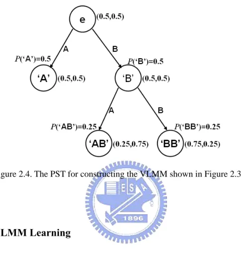
Figure 2.4. The PST for constructing the VLMM shown in Figure 2.3

2.3.1 VLMM Learning

The topology and the parameters of a VLMM can be learned from training sequences by optimizing the amount of memory required to predict the next symbol. Usually, the first step of training a VLMM involves constructing a prediction suffix tree (PST) [52]. A PST contains the information of the prefix of a symbol learned from the training data. Therefore, this prefix/suffix relationship helps to determine the amount of memory required to predict the next symbol. After the PST is constructed from the training sequences, the PST is converted to a PFSA representing the trained VLMM. Figure 2.4 depicts the PST constructed from a training sequence for converting the VLMM shown in

2.3 Variable-Length Markov Model

Figure 2.3.

Except for the root node, each node of the PST represents a non-empty symbol string, and each parent node represents the longest suffix tree of its child nodes. In addition, is the output probability distribution of the next symbol of each node s that satisfies

) |

(v s

P

v

∑

_v∈VP(v|s)= . The output and prior 1 probabilities can be derived from the training symbol sequences as follows

) ( ) ( ) | ( s N sv N s v P = , (2.11) 0 ) ( ) ( N s N s P = , (2.12)

where is the number of occurrences of string s in the training symbol sequences, and denotes the size of the training symbol sequences.

) (s

N

0

N

To optimize the amount of memory required to predict the next symbol, it is necessary to determine when the PST growing process should be terminated. Assume that s is a node with the output probability , and is its child node with the output probability . We choose a termination criterion in order to avoid degrading the prediction performance of the reconstructed VLMM. Note that if the child node’s output probability used to predict the next symbol, v, is significantly better than the output probability of the parent node, the child node is a deemed better predictor than the parent node; therefore,

) | (v s P v's ) ' | (v vs P (v P | (v P ) ' |vs ) s 25

Variable-Length Markov Model ) ' | (v v s P P(v|s)

the PST should be grown to include the new child node. However, if the inclusion of a new child node does not improve the prediction performance significantly, the new child node should be discarded. Usually, the weighted Kullback-Leibler (KL) divergence [10] is applied to measure the statistical difference between the probabilities and as follows:

∑

= Δ v P v s v v P | ( ' | ( log s s v v P s v P s s v H ) ) ) ' | ( ) ' ( ) , ' ( . (2.13)

If is greater than a given threshold, the node is added to the tree. In addition to the KL divergence criterion, a maximal-depth constraint of the PST is imposed to further limit the PST’s size.

) , ' (vs s H Δ v's

After the PST has been constructed, it must be transformed into a PFSA. First, the leaf nodes of the PST are defined as the states of the PFSA, and the latter’s initial probability function is defined according to the probabilities of leaf nodes. Then, the transition function can be defined according to the symbol string combined from leaf nodes and their prediction symbols. The output probability function is defined based on the output probability distribution of the next symbol of each leaf node. Finally, the PFSA can be derived from the PST. For example, Figure 2.3 shows the PFSA derived from a PST shown in Figure 2.4.

2.3 Variable-Length Markov Model

2.3.2 VLMM Recognition

After a VLMM has been trained, it is used to predict the next input symbol according to a variable number of previously input symbols. In general, a VLMM decomposes the probability of a string of symbols, O=o₁o₂...o_T, into the product of conditional probabilities as follows:

∏

= − − Λ = Λ T j j d j j o o o P O P j 1 1, ) | ( ) | ( , (2.14)

where oj is the j-th symbol in the string and dj is the amount of memory required

to predict the symbol oj.

The goal of VLMM recognition is to find the VLMM that best interprets the observed string of symbols, O=o₁o₂...o_T, in terms of the highest probability. Therefore, the recognition result can be determined as model * as follows:

i i ). | ( max arg * i O P i = Λ (2.15) 27

Chapter 3

Unsupervised Analysis of Human

Action Based on Manifold Learning

In this chapter, we describe the proposed framework for unsupervised analysis of long and unsegmented human action sequences based on manifold learning. First, we give an introduction about this research topic. The proposed approach is then described. Next, we detail the experiment results. Finally, conclusions are given.

3.1 Introduction

In general, unsupervised learning is more difficult than supervised learning, so the number of published unsupervised learning methods is much smaller than that of supervised ones. Wang et al. [65] proposed an unsupervised approach for analyzing human gestures. They segmented the sequences of a human motion into atomic components and trained an HMM for each atomic component. Then,

they applied a hierarchical clustering approach to cluster the segmented components using the distances between the HMMs. Based on the clustering result, each atomic action can be converted into a discrete symbol. Finally, they extracted behavior lexicons from discrete symbols using the COMPRESSIVE algorithm [43]. Zhong et al. [72] proposed an unsupervised technique for detecting unusual events in a large video set. First, the features of each frame in the video set were extracted and classified into prototypes using the k-means algorithm. Second, the video sequences were divided into equal length segments. Third, a segment-prototype co-occurrence matrix was computed so that the segments could be clustered using the document-keyword clustering method proposed in [18]. Finally, unusual video segments were identified by finding clusters far away from the others. Turaga et al. proposed a vocabulary model for dynamic scenes and presented algorithms for unsupervised learning of the vocabulary from long video sequences [59]. They first segmented a video sequence into action elements, each of which was modeled as a linear time invariant (LTI) dynamical system. Next, they clustered those segments to discover distinct action elements using the distances between the LTI systems [13]. Then each segment was assigned a discrete symbol, and persistent activities in the symbol sequence were identified by using n-gram statistics.

The above-mentioned approaches show that a general unsupervised system for human action analysis usually involves three stages: temporal segmentation, atomic action clustering, and atomic action learning and classification. Since the

3.1 Introduction

human shape can be modeled as an articulated object with a high degree of freedom, the dimensions of a human shape descriptor are usually very large. Under these circumstances, the computation required for temporal segmentation, clustering and classification in a high dimensional feature space is not intuitive and may be very time consuming. Theoretically, a continuous human action sequence can be viewed as the variation of human postures lying on a low-dimensional manifold embedded in a high-dimensional space, which can be learned effectively from a set of training data [36]. In this chapter, we propose a framework for unsupervised analysis of human action based on manifold learning. The goal of manifold learning, discussed in Section 2.2, is to discover a low-dimensional structure from a set of high-dimensional data. In recent years, some researchers have applied manifold learning algorithms to different tasks in the field of human action analysis, e.g., 3D body pose recovery [20], human tracking [41, 51], and human action recognition [12, 62]. The human action recognition methods proposed in [12, 62] are similar to the proposed approach, but they adopt a supervised learning method for human action recognition and they do not address the problems of temporal segmentation.

The main contribution of this study is that we propose a framework for unsupervised analysis of human action based on the Isomap algorithm. First, we propose a convex-hull shape contexts (CSC) descriptor to represent a human posture. Since the Isomap algorithm can preserve the CSC distance between any two postures of a training sequence and give a more faithful embedding,

mentioned in Section 2.2, we compute a CSC-based distance matrix and apply the Isomap algorithm to construct a low-dimensional structure from it. As a result, the training action sequence is mapped into a manifold trajectory in the Isomap space during the training process. To separate an action sequence into atomic actions precisely, the break points between any two consecutive atomic actions must be identified. To do this, we represent a manifold trajectory as a time series of low-dimensional points, and use a temporal segmentation technique to segment the manifold trajectory into atomic actions correctly. Next, we apply a DTW algorithm to perform atomic action sequence clustering. Finally, we use the clustered results to represent each cluster by an exemplar. For an input atomic action, we use the nearest neighbor rule to classify it into the correct category.

3.2 The Proposed Approach

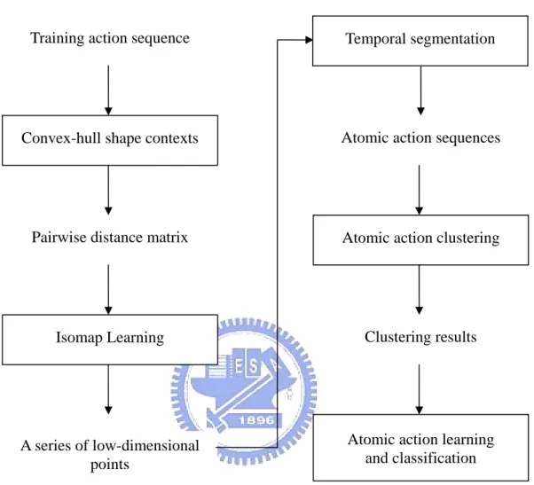
Figure 3.1 shows the flowchart of the proposed method. The proposed approach comprises five stages: Posture representation and matching, Isomap learning of human action, temporal segmentation, atomic action clustering, and atomic action learning and classification, which we describe in the following four subsections, respectively.

3.2 The Proposed Approach

Training action sequence

Convex-hull shape contexts

Pairwise distance matrix

Isomap Learning

A series of low-dimensional points

Atomic action sequences

Atomic action clustering

Clustering results

Atomic action learning and classification Temporal segmentation

Figure 3.1. The flowchart of the proposed method

3.2.1 Posture Representation and Matching

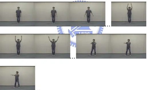
Human action usually consists of a series of discrete human postures, as shown in Figure 3.2. Therefore, a human posture can be represented by a silhouette image, and a shape matching process can be used to assess the difference between two postures. For simplicity, it is assumed that the input video sequence has been

processed to obtain the human silhouette sequence, i.e., the action sequence. To construct a low-dimensional structure of human action from a training action sequence, the human posture must be represented effectively in the high-dimensional space. Therefore in this work, we modify the shape context technique, discussed in Section 2.1, to represent the human posture and deal with the posture matching problem. This modified method is aimed to improve the efficiency of posture matching with the prerequisite of not sacrificing too much the matching accuracy.

…

…

…

Figure 3.2. Human action consists of a series of discrete human postures

Although the shape context matching algorithm usually provides satisfactory results, the computational cost of applying it to a large database of human postures is so high that is not feasible. To reduce the computation time, we only compute the local shape contexts at certain critical reference points, which should

3.2 The Proposed Approach

be easily and efficiently computable, robust against segmentation error, and critical to defining the shape of the silhouette. Note that the last requirement is very important because it helps preserve the informative local shape context. In this dissertation, the critical reference points are selected as the vertices of the convex hull of a human silhouette. Matching based on this modified shape context technique can be accomplished by minimizing a modified version of Equation (2.3) as follows:

∑

∈ = A p p q p C H'(π) ( , _{π( )})_{, (3.1)}

where A is the set of convex hull vertices and H′ is the adapted total matching cost. However, reducing the number of local shape contexts to be matched will also increase the influence of false matching results. To minimize the false matching rate, the ordering constraint of the vertices has to be imposed. However, since traditional bipartite graph matching algorithms [4] do not consider the order of all sample points, they are not suitable for our algorithm. Therefore, dynamic programming is adopted in the shape matching process. Suppose a shape P includes a set of convex hull vertices, A, and another shape Q includes a set of convex hull vertices, B. The CSC distance can be calculated as follows:

∑

∑

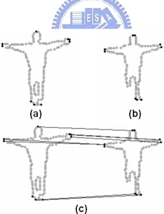
∈ ∈ + = B q q A p p C q p B q p C A Q P D_csc( , ) 1 ( , _{π( )}) 1 ( , _{π( )})_{. (3.2)}

An example of CSC matching is shown in Figure 3.3. There are three important reasons why convex-hull shape contexts can deal with the posture shape

matching problem effectively.

1. Since the number of convex hull vertices is significantly smaller than the number of whole shape points, the computation cost can be reduced substantially.

2. Convex hull vertices usually include the tips of human body parts; hence they can preserve more salient information about the human shape, as shown in Figure 3.2(a).

3. Even if some body parts are missed by human detection methods, the remaining convex hull vertices can still be applied to shape matching due to the robustness of computing the convex hull vertices, as shown in Figure 3.3.

Figure 3.3. Convex hull-shape contexts matching: (a) and (b) show the convex hull vertices of two shapes; (c) shows the correspondence between the convex hull vertices determined using shape matching.

3.2 The Proposed Approach

3.2.2 Isomap Learning of Human Action

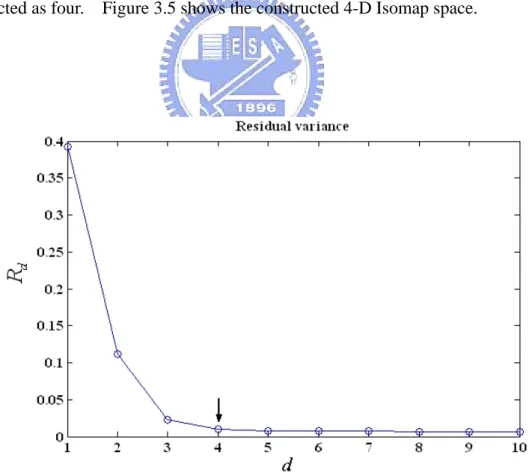
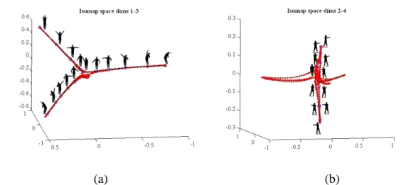
When each silhouette in the training action sequence is represented as a CSC descriptor, a pairwise shape distance matrix can be calculated based on the shape matching. The computed distance matrix is used to construct an Isomap using the method described in Section 2.2.1. As a result, each human silhouette is transformed into a low-dimensional point in the Isomap space. Figure 3.4 shows the residual variance of the Isomap on the training data computed with different values of d, from which the number of dimensions of the Isomap space can be selected as four. Figure 3.5 shows the constructed 4-D Isomap space.

Figure 3.4. The residual variance of Isomap on the training data

(a) (b)

Figure 3.5. The constructed 4-D Isomap space: the manifold trajectory of the action sequence projected on to (a) the first three dimensions (dims. 1-3), and (b) the last three dimensions (dims. 2-4).

3.2.3 Temporal Segmentation

The purpose of temporal segmentation is to identify suitable break points to partition a continuous action sequence into atomic actions. In Figure 3.5, it is obvious that different atomic actions that can be distinguished using the CSC descriptors will have different trajectories. Therefore, the segmentation process involves identifying the break points between any two successive atomic action trajectories. To deal with this problem, we first represent the manifold trajectory as a time series of d-D data points and then calculate the magnitude (i.e., the two norm) of each point, as shown in Figure 3.6. In general, a human motion slows down at the boundary of an atomic action. Therefore, the local minima and the local maxima of the magnitude series can be regarded as candidate break points. Furthermore, since humans usually return to a rest posture after completing an

3.2 The Proposed Approach

atomic action, we define the points that indicate low-speed actions and the postures adjacent to the rest posture as the break points of atomic actions. Note that, since rest postures appear in nearly almost all atomic actions, they are usually the most common postures mapped in the neighborhood of the origin of the Isomap space due to the zero-mean assumption formulated in Equation (2.7). Therefore, we only use the local minima as break points to derive atomic action sequences. In the magnitude series shown in Figure 3.6, there are eleven local minima, which divide the action trajectory into ten atomic actions.

Figure 3.6. The time series of data points and corresponding magnitudes after Gaussian smoothing