國 立 交 通 大 學
電控工程研究所
碩 士 論 文
適應性波束形成器於寬頻語音純化
使用具二階約束之卡曼濾波器
Adaptive Beamformer for Speech Enhancement
Using Second-Order Constrained Kalman Filter
研 究 生: 李 哲 宇
指導教授: 胡 竹 生 博士
適應性波束形成器於寬頻語音純化
使用具二階約束之卡曼濾波器
Adaptive Beamformer for Speech Enhancement
Using Second-Order Constrained Kalman Filter
研 究 生:李 哲 宇
Student: Che-Yu Li
指導教授:胡 竹 生 博士
Advisor: Jwu-Sheng Hu, Ph.D.
國立交通大學
電控工程研究所碩士班
碩 士 論 文
A Thesis
Submitted to Institute of Electrical and Control Engineering
College of Electrical Engineering
National Chiao Tung University
in partial Fulfillment of the Requirements
for the Degree of Master
in
Electrical and Control Engineering
July 2013
Hsinchu, Taiwan, Republic of China
適應性波束形成器於寬頻語音純化
使用具二階約束之卡曼濾波器
研究生:李 哲 宇
指導教授:胡 竹 生 博士
國立交通大學電控工程研究所碩士班
摘 要
當演算法中與環境及麥克風陣列的相關假設是不成立的時候,適應性波束形 成方法的性能會有大幅的衰減。當預設目標訊號出現在訓練的樣本數中,即使在 預設的指向向量和實際的指向向量有輕微的失配發生,陣列演算法的效果也會變 得相當靈敏,相關的失配問題發生於變動的環境以及遠近效應、聲源散佈、與局 部散射等。 本論文提出一套穩健型寬頻波束形成器,基於最佳化中在最糟情況下解決任 意且受規範的目標訊號之指向向量失配的問題。利用麥克風陣列訊號的空間資訊 ,由最小變異無失真響應(MVDR)的波束形成器以空間濾波的方式針對聲源方向 純化語音,同時壓抑來自於其它方向的雜訊。在實際應用的例子,波束形成器可 以表示為狀態觀測器於二階展開的卡曼濾波器(SOE-KF)。然而窄頻波束形成器沒 有考慮低頻訊號的空間指向性,目標聲源會因此受到壓抑而造成語音的失真。為 了在指向向量失配的情況下輸出較高的輸出訊號與干擾加雜聲比,演算法根據不 同頻帶下訊號的特性來選擇適當的指向向量的限制範圍。此外,當目標聲源不存 在時,演算法對雜訊做追蹤,並透過零波束形成限制式於 SOE-KF 中以進一步提 升語音純化的效果。本論文所提出的方法不僅改善了壓抑雜訊的效果並且提升了 語音的品質。透過模擬和實驗驗證,本論文所提出的演算法有效地提升語音品質 於吵雜以及有迴響的環境,並與其它已知的方法進行比較和分析。Adaptive Beamformer for Speech Enhancement
Using Second-Order Constrained Kalman Filter
Student: Che-Yu Li Advisor:Jwu-Sheng Hu, Ph.D.
Institute of Electrical and Control Engineering
National Chiao-Tang University
ABSTRACT
Adaptive beamforming methods are known to degrade significantly if some of underlying assumptions on the environment, sources, or sensor array are violated. The array performance may become sensitive even for a slight mismatch between the presumed and actual signal steering vectors when the desired signal is present. Such kind of mismatch occurs due to the dynamic environment, near-far mismatch, source spreading, and local scattering.
This paper presents a novel approach to design the robust broadband beamformer against arbitrary steering vector mismatch based on the optimization of worst-case performance. Using the spatial information from the microphone arrays, the desired source is enhanced while suppressing the directive noises via the robust minimum variance distortionless response (MVDR) beamformer. In practice, the beamformer is formulated into state-space observer form of the second-order extended (SOE) Kalman filter. However, the narrowband beamformer won’t consider the signal directivity in the low frequency-bands and the desired source would be distorted. For maintaining higher OutputSINR under steering mismatch, the broadband selection of the steering vector bound is investigated. Furthermore, the noise tracking is utilized as null constraints into the SOE Kalman filter for speech enhancement when the source is absent. The proposed algorithm in this thesis not only improves the performance of
noise suppression but also enhances the speech equality. Simulations and experiments demonstrate the effectiveness of the proposed algorithm in a noisy and reverberant environment by comparing with existing algorithms.
Index Terms—wideband beamformer, constrained Kalman filter, robust MVDR
beamformer, signal mismatch problem.
誌 謝
時光總是無形的流轉,很快地兩年的研究生涯要畫下句點了!過程中的點點 滴滴都將成為往後日子中無可取代的回憶。首先要感謝我的指導教授胡竹生老師, 謝謝老師給學生這個磨練自己的機會,在老師創新的思維的引導下,碰到困難的 時候學生學習獨立思考與解決研究問題的方法,跳脫舊有的模式,訓練自己具備 一位研究生該有的態度以及觀念,並對自己的研究內容負責。讓我以身為 XLAB 的成員感到驕傲,向老師獻上最誠摯的謝意。 另外感謝我的父母親家人們以及女朋友小璇,很多時候都能體諒我的無心抱 怨以及支持我做最好的自己,讓我無太多的後顧之憂,這些日子以來有你們的陪 伴和鼓勵,一直都是我努力向上的強力支柱。你們都是我最愛的人,感謝妳們相 信我的想法與目標,我一定不會讓你們失望的,謝謝妳們。 再來要感謝 XLAB 的成員們:文武雙全的唐哥,感謝您始終耐心地教導我許 多研究上的知識,祝您畢業後鵬圖大展;聲音組的棟樑耕維,祝您學業和事業一 切順利;實驗室最強的男人 Judo,大學專題中感謝有您領導一同奮戰的難忘時光, 祝您愛情與學業兩兩得意;兩年來室友兼戰友的罐頭,研究生涯中一同切磋知識, 謝謝您生活中大大小小不辭辛苦地幫忙,祝您愛情早日開花。還有率直的勁源學 長、理論基礎很扎實的阿吉學長、總是帶來驚喜和歡笑的阿法學長、專注和對理 想堅持的男哥、溫柔體貼的新好男人鳴哥、幽默風趣的廷哥、打球總是跳最高速 度最快的翰哥、社交能力一流的小山東,托你的福氣可以認識許多朋友、3C 產 品達人大夢,引領我進入蘋果的世界、毅力十足的阿文,認真的你最帥、研究專 注與謹慎的鳴遠、及總能跟上日韓潮流的期元、以及已經畢業的學長姐們和學弟 們,很榮幸加入 XLAB 這個大家庭,感恩大家對我的指導與包容。 最後要感謝交通大學,從大學到碩士生涯伴隨著我的回憶,提供許多學子進 修的管道以及資源,飲水思源的傳承是我往後受用無窮的做人本質,謝謝交大, 感謝在這裡的一切美好回憶。CONTENT
摘 要 ... I ABSTRACT ... II 誌 謝 ... IV CONTENT... V List of Figures ... VII List of Tables ... IX
Chapter 1. Introduction ... 1
1.1 Motivation and Objective ... 1
1.2 Literature Review ... 2
1.3 Thesis Scope and Contribution ... 4
1.4 Outline of Thesis ... 5
Chapter 2. Adaptive Beamformer ... 6
2.1 Array Signal Processing ... 6
2.2 Beamformer under MVDR Structure ... 10
2.3 Beamformer Using Equality State Constrained Kalman Filter ... 12
2.3.1 Soft-Constraint Kalman Filter under MVDR Structure ... 12
2.3.2 Hard-Constraint Kalman Filter under MVDR Structure ... 17
2.4 Adaptive Constrained Least Mean Square Beamformer ... 24
Chapter 3. Robust Adaptive Beamformer to the Signal Mismatch Problem ... 28
3.1 Introduction ... 28
3.2 Formulation of Signal Mismatch Problem ... 29
3.3 Solution to the Signal Mismatch Problem Using SOE Kalman Filter ... 33
3.4 Parameter Selection and Tradeoff ... 37
3.4.1 Covariance Matrix of Kalman Filter ... 37
3.4.2 Steering Vector Bound Wideband Selection ... 39
3.5.1 Beamformer Null Tracking when Source is Absent ... 45
3.5.2 Beamformer Null Constraint when Source is Present ... 50
3.6 Overall System Architecture ... 58
Chapter 4. Simulation and Experiment Results ... 61
4.1 Introduction of the Simulation and Experiment Condition ... 61
4.2 Adaptive Spatial Filter Comparison Result ... 66
4.3 Experiment on Performance to the Signal Mismatch Problem ... 71
Chapter 5. Conclusion and Future Study ... 86
List of Figures
Fig. 1 Uniform Linear Array structure (ULA). ... 7
Fig. 2 Uniform Circular Array structure (UCA)... 9
Fig. 3 Block diagram of the Soft-Constrained Kalman filter algorithm[12]. ... 16
Fig. 4 LMS algorithm block. ... 25
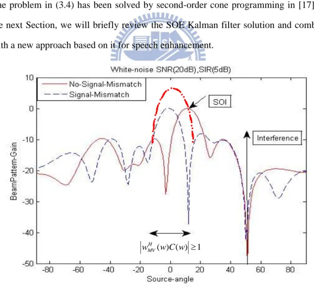
Fig. 5 Beampattern of signal mismatch and non-mismatch condition. ... 32
Fig. 6 (a) Output SINR of wideband epsilon selection ∆θ = 8𝑜(b) ∆θ = 16𝑜(SOE-KF). ... 39
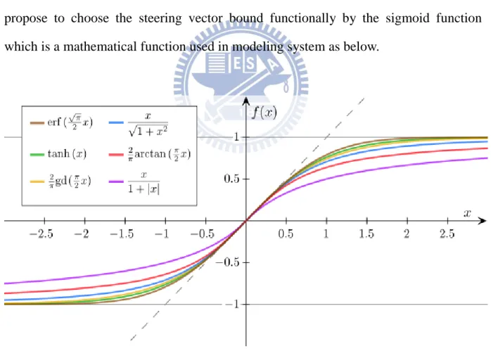
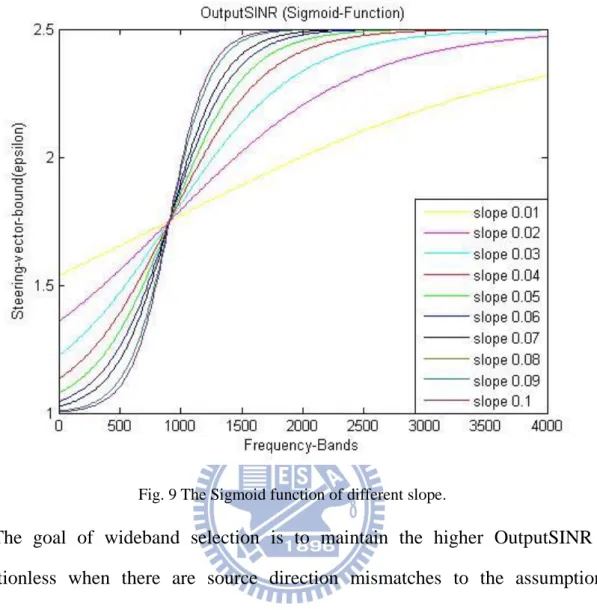
Fig. 7 The Sigmoid functions compared. ... 40
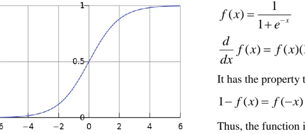
Fig. 8 Standard logistic sigmoid function. ... 41
Fig. 9 The Sigmoid function of different slope. ... 42
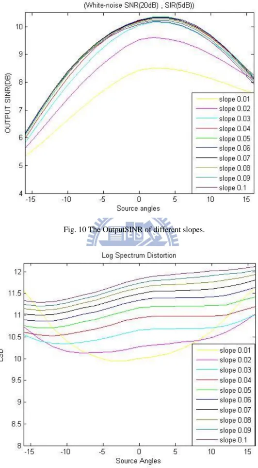
Fig. 10 The OutputSINR of different slopes. ... 43
Fig. 11 The Log Spectrum Distortion of different slopes. ... 43
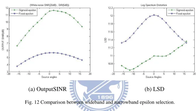
Fig. 12 Comparison between wideband and narrowband epsilon selection. ... 44
Fig. 13 (a) Wideband beampattern gain of one-interference 50𝑜(HC-KF)(b) (SOE-KF). ... 46
Fig. 14 (a) Wideband beampattern gain of two-interferences 50𝑜, −50𝑜(HC-KF)(b) (SOE-KF). ... 46
Fig. 15 Beampattern null tracking (two-interferences SIR 5(dB) 30𝑜, SIR 0(dB) 60𝑜). ... 49
Fig. 16 Beampattern null tracking (two-interferences SIR 5(dB) −50𝑜, SIR 5(dB) 50𝑜)... 49
Fig. 17 (a) Output SINR of null-constraint wideband epsilon selection ∆θ = 8𝑜(b) ∆θ = 16𝑜(HC-SOE-KF M=4). ... 52
Fig. 18 (a) Output SINR of null-constraint wideband epsilon selection ∆θ = 8𝑜(b) ∆θ = 16𝑜 (HC-SOE-KF M=6). ... 52
Fig. 19 (a) Peaks of OutputSINR with epsilon selection (no null-constraint) (b) null-constraint. ... 52
Fig. 20 Visible mainlobe of beampattern and bandwidth. ... 55
Fig. 21 (a) Delay and Sum (DAS) beamformer wideband beampattern M=4 (b) M=6. ... 56
Fig. 22 (a) Narrowband epsilon selection of one-interference 50𝑜(b) two-interference 50𝑜, −50𝑜(HC-SOE-KF). ... 56
Fig. 23 (a) Wideband epsilon selection of one-interference 50𝑜(b) two-interference 50𝑜, −50𝑜(HC-SOE-KF). ... 57
Fig. 24 (a) Narrowband epsilon selection speech enhancement of one-interference (b) two-interferences. ... 57
Fig. 25 (a) Wideband epsilon selection speech enhancement of one-interference (b) two-interferences. ... 57
Fig. 26 The Speech Enhancement structure of the Overall System. ... 58
Fig. 28 The location of microphone array and sources. ... 61
Fig. 29 Pre-processing of raw data in beamforming (STFT) ... 63
Fig. 30 The HATS and the digital microphone arrays (ULA). ... 64
Fig. 31 The real meeting room environment. ... 65
Fig. 32 The illustration of experiment equipments. ... 65
Fig. 33 The difference between SC-KF and HC-KF ... 67
Fig. 34 Comparison between different adaptive algorithms. ... 67
Fig. 35 Experiment results with input SNR 0(dB), SIR -7(dB). ... 68
Fig. 36 Experiment results with input SNR 0(dB), SIR 0(dB). ... 69
Fig. 37 Experiment results with input SNR 0(dB), SIR 7(dB). ... 70
Fig. 38 Comparison of mismatch conditions (No Null-constraint) (a) OutputSINR (b) LSD. ... 73
Fig. 39 Comparison of mismatch conditions (Null-constraint) (a) OutputSINR (b) LSD. ... 73
Fig. 40 Filtering results in different mismatch conditions (No Null-constraint). ... 74
Fig. 41 Filtering results in different mismatch conditions (Null-constraint). ... 75
Fig. 42 OutputSINR Comparison of algorithms (V+W). ... 77
Fig. 43 LSD Comparison of algorithms (V+W). ... 77
Fig. 44 PESQ Comparison of algorithms (V+W). ... 77
Fig. 45 Filtering results in input avgSINR -5(dB)(V+W) ... 78
Fig. 46 Filtering results in input avgSINR 0(dB)(V+W). ... 79
Fig. 47 Filtering results in input avgSINR 5(dB)(V+W). ... 80
Fig. 48 OutputSINR Comparison of algorithms (V+V). ... 82
Fig. 49 LSD Comparison of algorithms (V+V). ... 82
Fig. 50 PESQ Comparison of algorithms (V+V). ... 82
Fig. 51 Filtering results in input avgSINR -5(dB)(V+V). ... 83
Fig. 52 Filtering results in input avgSINR 0(dB) (V+V). ... 84
List of Tables
Table 1. Soft-Constraint Kalman filter algorithm. ... 16
Table 2. Hard-Constraint Kalman filter algorithm. ... 23
Table 3. Second-Order Extended Kalman filter algorithm. ... 36
Table 4. Second-Order Extended Constrained Kalman filter algorithm. ... 53
Table 5. Parameters in simulations and experiments. ... 62
Table 6. Results of different algorithms for speech enhancement based on MVDR(V+W). ... 76
Chapter 1. Introduction
1.1 Motivation and Objective
Speech enhancement in a noisy environment is an important research issue for speech signal processing. It will cause a great impact on both respects of voice recognition and communication. Although the hearing of human beings is able to recognize desired speeches even under noisy environment, it is still regarded as a difficult task for computers or machines.
The common sensor for receiving sound waves is the microphone. Single microphone can collect spectral information but not the spatial information. The advantage of microphone arrays is applied to catch not only spectral information but also spatial information among the sound waves. Adaptive spatial filter, which is called beamformer, is one of the most effective methods and are extensively studied for hands-free speech communication or recognition among several existing microphone-array-based speech enhancement algorithms in recent years.
The background noise and reverberation from undirected diffused noises or directed interferences are the most dominant reasons for the degradation of signal quality. The noises and reverberation level will determine the distortion level of the desired signal. Although the methods of multichannel speech enhancement are used to reduce the effect of noise and reverberation, they do not perform well in real practice when the pre-assumption of adaptive spectral filter violates the environment conditions. This provides the motivation of this thesis to study and propose innovative methods to handle both interference suppression and desired source mismatch problems, which is useful in a scenario like a real life conference in a meeting room or communication in the living room, where the equality of sound is deteriorated by human beings’ talking noise and reverberation in the space of the room.
1.2 Literature Review
Microphone arrays can be used to achieve the effect of spatial filtering, which is generally called Beamformer (BF) [1]. The beamformers can be categorized in two types, fixed beamformers and adaptive beamformers. Although the implementation costs of fixed beamformers are often lower than the adaptive beamformers, the beamforming effect is not robust enough due to there is no update mechanism in the algorithm.
Fixed beamformers include delay-and-sum beamformer (DAS) [2], constant directivity beamformer (CDB) [3] and fixed superdirective beamformers [4]. The fixed weights are utilized to form a spatial filter according to the pre-known spatial information. The DAS is the simplest structure in beamformer. It compensates to the relative time delay between distinct microphone signals and then sums the steered signals with a fixed weighting in every channel to form a single output. The CDB maintains the spatial response over a wide frequency-band; and the fixed superdirective beamformer keeps desired source distortionless at a pre-defined direction while attempting to suppress the noises from the other directions. These approaches assume the desired source and interferences are at pre-known location in stationary environment. Hence, these algorithms are sensitive to steering mismatches, which degrade the capacity of noise reduction and result to desired source distortion and signal self-cancellation.
Instead of using fixed beamformer, an adaptive beamformer can generate a beam response to the desired source direction and null at undesired signals to suppress the noises and interferences. Many adaptive beamformer techniques were extensively studied in the last three decade. The linearly constrained minimum variance (LCMV) beamformer was proposed in [5] to minimize the array output power under a look direction constraint. A special case similar to LCMV is the minimum variance
distortionless response (MVDR) proposed by Capon in [6]. Another popular technique is the generalized sidelobe canceller (GSC) algorithm which essentially transforms the LCMV constrained minimization problem into an unconstrained one [7].
The formulation of MVDR is implemented with Kalman filter using the state-space observer form. Owing to the undesirable mismatch between the actual desired signal steering vector and the presumed one in single steered constraint, various adaptive beamformers were proposed to improve the performance. The signal mismatches can be induced by signal point error [8], imperfect array calibration [9], or channel effect. In the presence of these effects, an adaptive beamformer suppresses the desired signal instead of maintaining distortionless response. Such phenomenon is commonly referred as signal self-nulling [10]. To strengthen the robustness against steering vector error, various methods are investigated [17], [19]. The Kalman filter can also be substituted by second-order extended Kalman filter [18], [20] and constrained Kalman filter [12], [13] to improve its robustness and reducing non-linearity against mismatch problems.
Among adaptive beamformers which are realized by Kalman filter, the usage of constraint projected method and steering vector bound regulation in wideband concept is a solution to the signal mismatch problem. The relative theory can be found in [17], [18], [21], [22].
1.3 Thesis Scope and Contribution
The contribution of this thesis is to propose and implement an innovative algorithm against signal mismatch problem for speech enhancement. The scope of thesis can be divided to two parts. The first part is to formulate a constrained adaptive beamformer considering the multiple arrays directivity and spatial coherence of spatial filtering. The second part is to handle the beamforming constraints given by the information of voice activity detection to achieve better performance of speech enhancement.
In the first part, the formulation using MVDR structure with signal mismatch problems is given. To obtain the solution, the nonlinear second-order extended Kalman filter is applied to deal with inequality nonlinear constraints as well as constraining the state prediction. In the optimal minimum mean-square error (MMSE) algorithm, the selection of parameters is to avoid suppression of the desired signal component (signal self-nulling) in broadband sense. Each selection has different result in different signal mismatch situation. The principle of selection is investigated and explained.
In the second part, the noise tracking can be utilized as null constraints for further enhancement when the desired source is not present. We incorporate the equality-constraints (Hard-Constraints) into the Kalman filter by projecting the updated state estimate onto the constrained region. The robustness of performance against signal mismatch for directive noise and dereveberation is achieved by choosing appropriate parameters in different conditions (ex: microphone arrays number, mismatch angle). In particular, the information given by the voice activity detector can also be reused to select appropriate parameters in beamforming. The performance of the algorithm is discussed and explained.
1.4 Outline of Thesis
The remainder of this thesis is organized as follows.
Chapter 2: The beamformers of adaptive spatial filtering which are based on the robust beamforming technique Minimum Variance Distortionless Response (MVDR) are introduced. The ideal steered linear inequality constraint is incorporated into the steepest gradient method and state space formulation to implement MVDR. By comparisons, the pros and cons construct the foundation of proposed algorithm.
Chapter 3: The detailed formulation of second-order extended Kalman filter with nonlinear inequality constraints is presented. It includes the solutions to signal mismatch problem and beamformer null constraint for suppression of interferences, given the information of voice activity detection (VAD). The technique of choosing the appropriate parameter in wideband beamforming and its effect are also discussed. Finally, the overall flowchart and architecture are illustrated and explained.
Chapter 4: The results of simulation and experiment are shown. It contains comparison between adaptive spatial beamformers and the capability of beamforming against signal mismatch problem in Room Impulse Response (RIR) and real room respectively. Some objective indices are calculated to compare the performance between proposed algorithm and other existing algorithms. Chapter 5: The conclusion of this thesis and some issue that is discussed for future
Chapter 2. Adaptive Beamformer
2.1 Array Signal Processing
In the traditional digital signal processing, Most of the techniques focus on the processing skills in the time and frequency domain. Generally, sampling the continuous signals first, and then converting to the frequency domain to analyze the signals or discriminate different components by passing the filter.
Multiple microphones are in a fixed shape to receive the signals which are transported in the spatial. As a result of the microphones in the different position, microphones will retrieve different energy change and time delay from the same signal in the same source. Then the processing analysis for exacting a desired source out of spatial distinct sources from multiple microphones is called microphone array signal processing. The field of the research can be classified to two categories:
First
:Focus on the number of signals or the spatial direction, generally called (Direction of Arrivals Estimation, DOA).Second
:Using the spatial relationship of signals can find out different gain of different direction of signals to have the spatial filtering effect. Generally, theway to separate the different direction signals is beamformer, and is also one kind of spatial filter.
Assign a microphone array and a reference point (generally one microphone of the array), array manifold vector defines the relationship between the source signal retrieved from microphones and the reference point of time. In the thesis of beamformer, array manifold vector is used to compensate the input signal phase delay between different microphones. And, in the thesis of Direction of Arrivals Estimation,
many methods find out the source direction by comparing the similarity of array manifold vector and the eigenspace of source signals (Eigenstructure Method DOA). The array processing converts the raw data into frequency domain to compute by Short-Time Fourier Transform (STFT). In frequency domain, the time delay will become to the phase delay. Thus, the resolution of computation for source angle improves effectively in frequency domain.
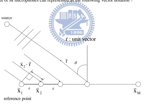
Usually using the different array arrangement in different situation, following is the common (Uniform Linear Array, ULA). The structure is as Fig. 1. Assume the source signal is the (Far field plane wave), s(t) is initial source, n(t) is noise, and the output of M microphones can represented as the following vector notation:
Fig. 1 Uniform Linear Array structure (ULA).
This Thesis is based on the Uniform Linear Array structure.
d d source
r
r : unit vector
reference point 1x
x
2x
M 2x
r
1 1 1 1 2 1 ( ) ( ) ( ) ( ) ( ) ( ) ( ) ( ) ( ) ( ) ( ) ( ) ( ) c M c M c c x r jw c x r j jw M c x r x r M k jk x t s t e n t x t x t n t s t e n t a r s t n t n t e s t e (2.1) 2 c c c w k c
, kc is called wavenumber, and wc is the wavelength, c is the
wavespeed.
( )
a r is the array manifold vector, including the time relationship of signals transported to the microphones, which can simplified as following :
sin (M 1)sin
( )
1
jk dc jkcT
a
e
e
(2.2)In addition to the assumption to the source model, the equality of the microphones has to be checked to a certain extent. Theoretically, we will assume the characteristics between microphones are identical completely (No difference in gain or phase) to ensure the signal from desired source to the microphone arrays is just a relationship of time delay. Once there is difference between arrays, the estimation of spatial equivalent relationship will be influenced considerably (ex, Direction of Achieving Angle). Therefore, we have to confirm the gain between microphones is limited to a range. When the distance from desired source to microphone arrays is smaller, we have to consider the near-field assumption. Opposite to the near-field assumption is the far-field assumption which is used in array signal processing. Moreover, the shadowing effect of arrays disposal and directivity of array itself will both influence the spatial relationship that arrays received.
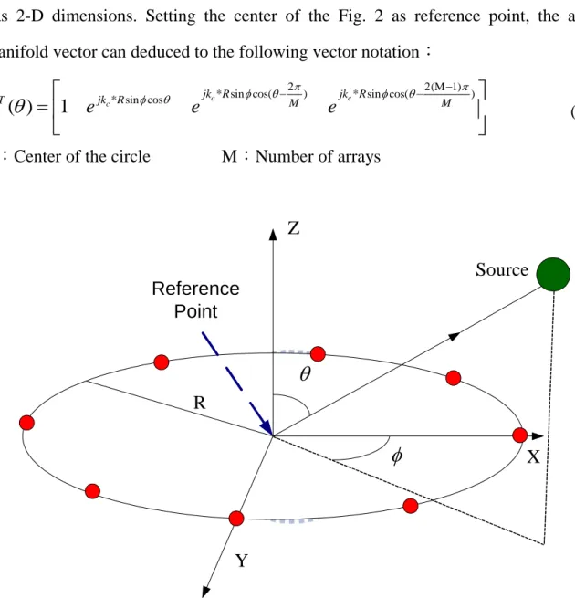
Fig. 2 is the uniform circular array arrangement. Its source angle searching ability has 2-D dimensions. Setting the center of the Fig. 2 as reference point, the array manifold vector can deduced to the following vector notation:
2 2(M 1)
* sin cos( ) * sin cos( ) * sin cos
( )
1
c c c jk R jk R jk R T M Ma
e
e
e
(2.3)R:Center of the circle M:Number of arrays
Z X Y
R Source Reference Point2.2 Beamformer under MVDR Structure
The minimum variance distortionless response (MVDR) beamformer, also known as Capon beamformer [6], minimizes the output power of the beamformer under a single linear constraint on the response of the array towards the desired signal.
Consider the conventional signal model in which an M-element microphone array captures a convolved desired signal (speech source) in some noise field. The received signals are expressed as [3]
xm(k)am*s(k)vm(k) m1 , 2 , . . . M (2.4) where am is the impulse response from the unknown (desired) source s(k) to the
th
m microphone, * stands for convolution, and vm(k) is the noise at the microphone
m. The signals s(k) and vm(k) are assumed as uncorrelated and zero mean. In the frequency domain, (2.4) can be written as
Xm(jw)Am(jw)*S(jw)Vm(jw) m1 , 2 , . . . M (2.5) where Am( jw), S( jw), Xm( jw), Vm( jw) are the discrete-time Fourier transforms (DTFTs) of am(k) , s(k) , xm(k) , vm(k) , respectively, at angular frequency
) (
w
w and j is the imaginary unit ( j2 1).
These M microphone signals in the frequency domain are summarized in a vector notation as ) ( ) ( ) ( ) (jw A jw S jw V jw X (2.6) where 1 2 1 2 1 2 ( ) [ ( ) ( ) ( )] ( ) [ ] T X A [ ] V T M M T M jw X jw X jw X jw (jw) A (jw) A (jw) A (jw) jw V (jw) V (jw) V (jw) and superscript T
Consider finding a weighting vector wMV which satisfies the look direction constraint ( ) ( , ) 1 H MV s w jw a jw (2.7) while attempting to minimize beamformer output power
2 2
{ ( ) } { MVH ( ) ( ) } MVH ( ) XX( ) MV( )
E Y jw E w jw X jw w jw R jw w jw (2.8) in order to suppress undesired interference from s and noise. Y( jw) is the beamformer output given by
(jw)wMVH (jw X jw) ( )
Y . (2.9)
( ,s )
a jw is the array manifold vector that points to the source direction.
With the consideration above, the following constrained optimization problem can be formulated:
minwMVH (jw R) XX(jw w) MV(jw) subject to wMVH (jw a) ( ,s jw) 1 (2.10) To solve this problem, the Lagrange Multiplier is incorporated.
( ) ( ) ( ) ( ) ( )[ ( ) ( , ) 1] 0 ( ) ( , ) 1 MV MV H H W jw MV XX MV W jw MV s H MV s w jw R jw w jw w jw a jw w jw a jw (2.11) (2.8) can be reduced to ( ) ( ) ( , ) ( ) ( , ) 1 XX MV s H MV s R jw w jw a jw w jw a jw (2.12)
Assuming RXX is nonsingular. Then 1 1 ( ) ( , ) ( ) ( , ) ( ) ( , ) XX s MV H s XX s R jw a jw w jw a jw R jw a jw (2.13)
2.3 Beamformer Using Equality State Constrained Kalman Filter
Kalman filtering [26] is a method to make real-time prediction for systems with some known dynamics in control theory. Traditionally, problems requiring Kalman Filtering have been complex and nonlinear. Many advances have been made in the direction of dealing with nonlinearities (e.g., Extended Kalman Filter, Unscented Kalman Filter). These problems also tend to have inherent state space equality constraints and state space inequality constraints. In this thesis, the use of constrained Kalman filter in signal processing is more concerned. A constraint on the microphone array response along the look direction is added to the measurement equation of the Kalman filter. The weight vector of the constrained Kalman beamformer is derived and shown to converge to that of the minimum-variance distortionless-response beamformer (MVDR). The technique of incorporating state space concept and Kalman filter to solve the MVDR problem is presented in subsection 2.3.1 and subsection 2.3.2 by two forms of constraints. In later Sections, another formulation to maintain the distortionless constraint will be presented and investigated.
2.3.1 Soft-Constraint Kalman Filter under MVDR Structure
The traditional formulation and solution to MVDR is presented in Section 2.2. In this Section, The Kalman filter is introduced to solve the MVDR problem in a new formulation by Y.H. Chen and C.T. Chiang [12].
With the same formulation as MVDR structure above(2.10), state equations describing such formulation can be written as:
Measurement Equation: 1 2 0 ( , ) ( , ) ( , ) ( , ) ( , ) ( , ) ( ) 1 ( , ) ( , ) H H H s s v k jw X k jw w k jw k jw w k jw k jw f a jw v k jw Y X V (2.14) Process Equation ( 1, ) ( , ) ( , ) w k w w k w Q k w (2.15)
where k is the frame index and the superscript “H” means conjugate-transpose. A
cure for the signal-distortionless problem is to constrain the gain of the system as unity on the desired signal from look direction and minimize the system output power subject to this constraint as Equation (2.7). The noise V(k,w) and Q(k,w) are assumed with Gaussian distribution and thus the covariance matrix can be written as
2 2 1 2 2 ( , ) ~ (0, ) 0 ( , ) ~ (0, ) 0 Q v v k w N I k w N Q V (2.16)
where “N” means Normal Distribution and 2
Q , 2 1 v , 2 2 v
are parameters to be chosen.
( , )k w
X is the received signal and a( ,s jw)is the array manifold vector.
Let the state estimation error is
ˆ
( 1, ) ( , ) ( 1, )
e k k w w k w w k k w (2.17) and the error covariance matrix is
( 1, ) [ ( 1, ) T( 1, )]
ee
R k k w E e k k w e k k w (2.18) In the first step, no new observation is used. To predict w k( ) by using the state
equation, the best possible predictor would be as below which is given that no new information is available.
w k kˆ( 1, )w w kˆ( 1k1, )w (2.19) The estimation error is
ˆ ( 1, ) ( , ) ( 1, ) ˆ ( 1, ) ( , ) ( 1 1, ) ( 1 1, ) ( , ) e k k w w k w w k k w w k w Q k w w k k w e k k w Q k w (2.20)
constant bias in the optimal linear estimation [7]), E e k k[ ( 1, )]w 0. Since ( 1 1, ) e k k w is uncorrelated with Q(k,w), 2 ( 1, ) ( 1 1, ) ee ee Q R k k w R k k w I(Riccati Equation) (2.21)
In the second step, the new observation, 0
( ) 1s
f
=Y(k,w) is incorporated to estimatew(k,w). A linear estimate that is based on w k kˆ ( 1, )w and Y(k,w) has the form
ˆ( , ) '( , ) (ˆ 1, ) ( , ) ( , )
w k k w K k w w k k w k k w Y k w (2.22)
where K'(k,w) and k(k,w) are some matrix and vector to be determined. The vector
) , (k w
k is called the Kalman gain. Now, the estimation error is
ˆ ( , ) ( , ) ( , ) ˆ ( , ) '( , ) ( 1, ) ( , ) ( , ) ( , ) '( , )[ ( , ) ( 1, )] ( , )[ ( , ) ( , ) ( , )] [ '( , ) ( , ) ] ( , ) '( , ) ( 1, ) ( , ) ( , H H k k w w k w w k k w w k w k w w k k w k w k w w k w k w w k w e k k w k w k w w k w k w I k w k w w k w k w e k k w k w k w e K k Y K k X V K k X K k V ), (2.23) where ( , ) ( , ) ( , ) H H H s X k w k w a jw X .
Since E e k k[ ( 1, )]w 0, then E e k k w[ ( , )]0 only if
'( , )k w I ( , )k w H
K k X (2.24) with this constraint, it follows that
ˆ( , ) [ ( , ) ] (ˆ 1, ) ( , ) ( , ) ˆ ˆ ( 1, ) ( , )[ ( , ) ( 1, )] H H w k k w I k w w k k w k w k w w k k w k w k w w k k w k X k Y k Y X (2.25) and ( , ) '( , ) ( 1, ) ( , ) ( , ) [ ( , ) H] ( 1, ) ( , ) ( , ). e k k w k w e k k w k w k w I k w e k k w k w k w K k V k X k V (2.26)
Since V(k,w) is uncorrelated with Q(k,w) and with Y(k1,w), then V(k,w) will be uncorrelated with w k w( , ) and with w k kˆ ( -1, )w ; as a result E e k k w[ ( , ) ( , )]V k w =0. Therefore, the error covariance matrix for e k k w( , ) is
( , ) [ ( , ) ( , )] [ ( , ) ] ( 1, )[ ( , ) ] ( , ) ( , ) ( , ), T ee H H T T ee v R k k w E e k k w e k k w I k w R k k w I k w k w R k w k w k X k X k k (2.27) where R k wv( , ) = 2 1 1 0 0 v v .
The final task is to find the Kalman gain vector k(k,w), that minimizes the MSE
( ) [ ee( , )]
J k tr R k k w (2.28) Differentiating J(k) with respect to k(k,w), we get
( ) 2[ ( , ) ] ( 1, ) 2 ( , ) ( , ) ( , ) H ee v J k I k w R k k w k w R k w k w k k X X k (2.29)
and equating it to zero, we deduce the Kalman gain
1 ( , )k w Ree(k k 1, )w HRee(k k 1, )w R k wv( , ) k X X X (2.30)
The expression for the error covariance matrix can be simplified as
( , ) [ ( , ) ] ( 1, ) [ ( , ) ] ( 1, )[ ( , ) ] ( , ) ( , )} ( , ) H ee ee H H T ee v R k k w I k w R k k w I k w R k k w I k w R k w k w k w { , k X k X k X k k (2.31)
Where, by using (2.29), the second term in (2.31) is equal to zero. Hence
( , ) [ ( , ) H] ( 1, )
ee ee
R k k w=Ik k wX R k k w (2.32)
In conclusion, the Soft-Constraint Kalman filter can be summarized as following. The signal-flow graph of the constrained Kalman algorithm can be plotted as Fig. 3.
Algorithm: Soft-Constraint Kalman filter
Table 1. Soft-Constraint Kalman filter algorithm.
Fig. 3 Block diagram of the Soft-Constrained Kalman filter algorithm[12].
State Equation:
ˆ( 1 , ) ˆ( , ) ( , )
w k k w w k k w Q k w
Measurement Equation (Cost Equation):
0 ( , ) ( , ) ( , ) ( , ) ( ) 1 ( , ) H H s s X k w k w w k w k w f a jw Y V =XH( , ) ( , )k w w k w V( , )k w Computation for k 1,2, ˆ( 1, ) ˆ( 1 1, ) w k k w w k k w 2 ( 1, ) ( 1 1, ) ee ee Q R k k w R k k w I
The Kalman gain:
1 ( , )k w Ree(k k 1, )w HRee(k k 1, )w R k wv( , ) k X X X ˆ( , ) ˆ( 1, ) ( , )[ ( , ) H( , ) (ˆ 1, )] w k k w w k k w k k w Y k w X k w w k k w ( , ) [ ( , ) H( , )] ( 1, ) ee ee R k k w I k k w X k w R k k w
Soft equality constraints are constraints that are only required to be approximately satisfied rather than exactly satisfied. The perfect measurement approach (Kalman- Filter) can be extended to soft constraints by adding small nonzero measurement noise to the perfect measurement as v. It makes the optimal Lagrange Multiplier solution be a trade-off between the residual error and the constraint error. The methods are implemented in cases where the constraints are heuristic rather than exactly satisfied. But in thesis cases, we want to use Hard-constraints, as opposed to Soft-constraints, to solve the signal mismatch problem which is discussed in next Chapter.
2.3.2 Hard-Constraint Kalman Filter under MVDR Structure
A number of approaches have been proposed for solving the constrained Kalman Filtering problem [13], [14], [15], [26]. Analogous to the way that a Kalman filter can be extended to solve problems containing nonlinearities, linear equality constrained filtering can be extended to problems with nonlinear constraints by linearizing locally. The accuracy achieved by methods dealing with nonlinear constraints will naturally depend on the structure and curvature of the nonlinear function itself. We would want to implement the equality constraints that are exactly satisfied specifically.
In this subsection, there are two distinct approaches which are discussed to generalize an equality constrained Kalman Filter. The first approach is to run an unconstrained Kalman Filter and project the estimate down to the equality constrained space in each iteration. The second approach will start with a constrained prediction, and restrict the Kalman Gain so that the estimate will lie in the constrained space. Finally, we will show the numerical preservation of the updated error covariance with the feedback loop in the projection framework. The equality constraint in this subsection can be defined as below, whereAis a q w matrix, b is a q-vector, and
k
( k)
A w b (2.33) So the updated state estimate and state prediction to be constrained at each iteration, which would allow a better forecast in the system, as below.
| | 1
ˆ
{
k k k kAw
b
Aw
b
state estimatestate prediction
(2.34) In the following two approaches, we will discuss the constraining updated state estimate.
A. Projecting the Unconstrained Estimate
This method projects the state to lie in the constrained space each iteration, feeds the new constrained estimate back to the unconstrained Kalman Filter and continues this process. Such method can be described by the following minimization problem for a given time-step k, in which ˆP|
k k
w is the constrained estimate, wˆk k| is the unconstrained estimate from the Kalman Filter equation, and Wkis any positive definite symmetric weighting matrix, where the superscript ‘P’ is used to denoted the
“Projected” constrained filter and ‘U’ is denoted as “Unconstrained”.
| | | ˆ arg min ( ˆ ) ( ˆ ) : n P U T U k k k k k k k w w w w W w w Aw b (2.35) The constrained estimate is then solved by the Lagrange Multiplier as equation (2.11~2.13), which is given as below:1 1 1
| | |
ˆk kP ˆUk k k T( k T) ( ˆUk k )
w w W A AW A Aw b (2.36)
In a general case, we can find out the updated error covariance as a function of the unconstrained Kalman Filter’s updated error covariance matrix as before. Define the matrix as below first.
1 ' 1 ' 1
( )
k k
W A AW A
Equation (2.36) can be re-written as follows:
| | |
ˆk kP ˆUk k ( ˆUk k )
w w Aw b (2.38) The reduced form for ˆP|
k k k w w as below: | | | | | | ( )( ˆ ˆ ( ( )) ˆ ˆ ) ( ) ˆ P k k k k k k k k k k k k k k k k k k w w w w Aw b Aw b w w A w w A w w I (2.39)
According to the definition of the error covariance matrix, we arrive at the following expression. ' | | ' ' | | ' | ' ' ' ' | | | | | | | | ( )( )( ) ( ) ( ) ( ) ( ˆ ˆ ( )( ) ) ˆ ˆ I k k k k k k k k k k k k k k k k k k k k k P P P k k k k k k k k k P E w w w E I A x x I A I A P I A P AP P A AP A P AP A P w w w (2.40)
Note that the A in equation (2.39) is a projection matrix, as is(I A), so we can deduce the equation (2.40) to the result. It can be shown that there is smallest updated error covariance when 1
|k
k k
W P . It also provides a measure of the information in the state k.
B. Restricting the optimal Kalman Gain
Alternatively, for restricting the optimal Kalman gain so the updated state estimate lies in the constrained space, we can expand the updated state estimate term in Equation (2.34) using Equation (2.25), the state update is wˆk k| wˆk k| 1K Vk k, where
| 1 ˆ ( ) k k k k k V Y H w . | 1 ˆ ( k k k k) A w K V b (2.41)
The MMSE of the estimate wˆk k| isE(wkwˆk k| ) (T wkwˆk k| ), which is equivalent
to the trace of error covariance matrix of wˆk k| . Then, we can choose a Kalman Gain
P k
K that forces the updated state estimate to be in the constrained space. We choose the optimal Kalman Gain Kk which yields Equation (2.30) in the unconstrained case by solving the minimization below
* ' ' | 1 arg min ( ) ( ) n m k k k k k k k k k k K K trace I K H P I K H K R K (2.42)
Now we seek the optimal P k
K that satisfies the constrained optimization problem written below for a time-step k.
* 1 ' ' | 1 | . arg m . ( ) in ( ) ( ) ˆ n m P k k k k k k k k k k k k k K K trace I K H P I K H K R w s K t A K V b (2.43)
Using the method of Lagrange Multiplier technique to solve the optimal minimization, ' 1 | 1 ' | (( ) ( ( ( ) ) ) ˆ ) k k k k k k k T k k k k k k k k J Tr I K H P I K H K R K A w K V b (2.44)
where the k is the Lagrange multiplier. Taking the derivative of Jk with respect to
k
K and setting it to zero yields
| 1
2Pk k HkT 2K Ck k AkT
kVkT 0 (2.45)
where | 1 T
k k k k k k
C H P H R . Then we find the following Kalman gain.
1 1 | 1 1 2 P T T k k k k k k k k T k K P H C A
V C (2.46) Applying Equation (2.41), after some manipulations, the optimal Lagrange multiplier is obtained as below.1 1 1 | 1 | 1 2( T T) ( T T ˆ ) k V C V A Ak k k k k A Pk k k H C Vk k k A wk k k b (2.47)
Finally, substituting the optimal Kalman Gain and Lagrange multiplier into the Equation (2.41) that yields the following constrained updated state estimate:
1 |
ˆ
k kP Uk kT(
k kT) (
kˆ
Uk)
w
v
A
A A
A w
b
(2.48) This is of course equivalent to the result of Equation (2.36) with the weighting matrixk
W which is chosen as the identity matrix in open loop scheme. The error covariance is given by Equation (2.40). That is, the Kalman Filter can be run in real-time, and as a post-processing step, the unconstrained estimate and updated error covariance matrix can be reformulated in the constrained space; or alternatively, the constrained estimate and its updated error covariance matrix can be fed back into the system in real-time. A large benefit of incorporating constraints can be realized in both techniques, though the feedback system should generally outperform the system without feedback.
Numerical Preservation of the Updated Error Covariance
These methods are shown to be mathematically equivalent under the assumption
that the weighting matrix Wk is chosen appropriately. In [15], with the augmentation method, the soft equality constraints can be deduced to be equivalent to hard equality constraints into a Kalman filter by adding a proportionate amount of noise to the bottom right error covariance matrix (see Equation (2.16)). However, the numerical round-off error will be ignored possibly in implementations. We will not see the exact same result while these methods can be mathematical equivalent. The round-off error that causes the most trouble occurs when the updated error covariance matrices lose symmetry or positive definiteness. According to feedback loop of the projection frame, we should find a form of state estimate and state error covariance that preserves symmetry and positive definiteness better.
[15] uses the numerical preservation of updated error covariance to find a simplified form for the constrained updated error covariance as below:
' '
| ( ) | 1( )
P P P U P P P P
k k k k k k k k k k k
P I K H P IK H K R K (2.49) Define the projection matrixk,
' ' 1 | ( | ) U U k I P A AP Ak k k k A (2.50) In term of k, the following are true.
| | | | | | { ( ) P U k k k k k P P P P k k k k k k k k k P P I K H I K H (2.51) Finally, in order to maintain numerical stability we can find out the simplified form of constrained updated error covariance by using Equation (2.49).
' ' | | 1 ' ' | 1 ' ' ' ' ' | 1 ' | ( ) ( ) ( ) ( ) ( ) ( ) P P P U P P P P k k k k k k k k k k k U U U U U k k k k k k k k U U k k k k k U U U U U U U k k k k k k k k k k k U k k k k P I K H P I K H K R K I K H P I K H K R K I K H P I K H K R K P (2.52)
In conclusion, the Hard-Constraint Kalman Filter can be summarized under MVDR structure as following :
Algorithm: Hard-Constraint Kalman filter
Table 2. Hard-Constraint Kalman filter algorithm.
State Equation:
ˆ( 1 , ) ˆ( , ) ( , )
w k k w w k k w Q k w
Measurement Equation (Cost Equation):
( , )k w 0 H( , ) ( , )k w w k w ( , )k w Y X V Computation for k 1,2, ˆ( 1, ) ˆ( 1 1, ) w k k w w k k w 2 ( 1, ) ( 1 1, ) ee ee Q R k k w R k k w IThe Kalman gain :
1
( , ) ee( 1, ) H ee( 1, ) v( , )
k k w R k k w X X R k k w XR k w
Update the state estimate :
ˆ( , ) ˆ( 1, ) ( , )[ ( , ) H( , ) (ˆ 1, )]
w k k w w k k w k k w Yk w X k w w k k w
1
ˆ( , ) ˆ( , ) H( ,s )( ( ,s ) H( ,s )) ( H( ,s ) (ˆ , ) )
w k k w w k k w a jw a jw a jw a jw w k k w b
Update the error covariance :
( , ) [ ( , ) H( , )] ( 1, ) ee ee R k k w I k k w X k w R k k w 1 1 ' ( , ) [ ( , )( ( , ) ( , )) ( , )]* ( , )[ ( , )( ( , ) ( , )) ( , )] H H ee s s s s H H ee s s s s R k k w I a jw a jw a jw a jw R k k w I a jw a jw a jw a jw b: Response value
2.4 Adaptive Constrained Least Mean Square Beamformer
The optimal Linearly-Constrained Minimum-Variance Filter (LCMV) in the concept of the minimum mean output energy (MOE) that minimizes the same objective function as MVDR beamformer, and projects to the set of the linear constraints. In [5] Frost has proposed an algorithm to estimate wopt based on the least-mean-square (LMS) algorithm for adaptive filtering. Under the MVDR structure, linearly-constrained adaptive filters are deduced as below.
Core of the LMS algorithm is to find a weighting to minimize the error covariance between desired source and filtered output. Assume the desired signal, that we want to achieve, is zero-mean and the variance is 2
d
. Auto-correlation and cross-correlation matrices definition of the input signal are the following.
2 2 * Auto correlation ( matrix ) 0, ( ) ( ) * ( )d( ) ( ) Cross correlation matrix
d xx dx E d k E d k R E x k x k R E k x k Then the Cost function is as Equation (2.53).
2 *( ) min ( ) ( ) * ( ) ( ( ) ( ) * ( ))( ( ) ( ) * ( ))
w
J k E d k x k w k E d k x k w k d k x k w k (2.53)
Then the method to find the weighting is the Steepest-Descend Method as
( ) ( 1)
w k w k p (2.54) is the proportion called step-size (or convergence factor), and the p choosing is deduced from (2.53). Expanding the Equation (2.53):
2 * * *
( ) d dx ( ) ( ) dx ( ) xx ( )
J k R w k w k R w k R w k (2.55) We take the w of (2.55) to find the minimization and we get
( 1)
dx xx
pR R w k , (2.56) For the purpose to let w k( )on the lowest direction and strength of J k( ),
and rewritten the (2.54)
( ) ( 1) dx xx ( 1) 1
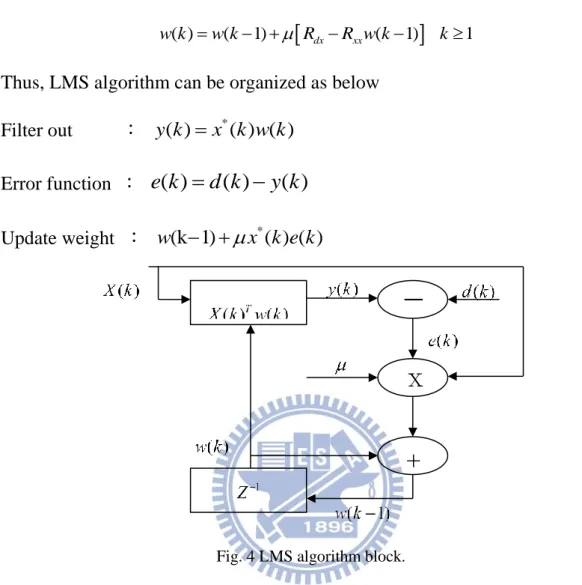
w k w k R R w k k (2.57)
Thus, LMS algorithm can be organized as below Filter out : y k( )x k w k*( ) ( )
Error function :
e k
( )
d k
( )
y k
( )
(2.58) Update weight : w(k 1)
x k e k*( ) ( )Fig. 4 LMS algorithm block.
Since the frequency response of look-direction is fixed by the desired source constraint under MVDR structure, minimization of the non-look-direction noise power is the same as minimization of the total output power as Equation (2.10). The gradient-descent constrained LMS algorithm presented as below using the same method of Lagrange multipliers, which is discussed in Equation (2.11).
( ) ( 1) ( 1) ( 1) ( 1) ( ) ( ) w xx s w k w k H w k w k R w k a k (2.59) The Lagrange multipliers are chosen by requiring w k( )to satisfy the constraint( )s T( ) ( )s T( ) ( )s T( )s xx ( ) T( ) ( ) ( ) 1s s
f a w k a w k a R w k a a k (2.60) Solving for the Lagrange multipliers ( )k and substituting back to the weight
+
-
iteration Equation (2.59), 1 1 (k) ( 1) ( )( ( ) ( )) ( ) ( ) (k) ( )( ( ) ( )) ( ) 1 ( ) (k) T T s s s s s xx T T T s s s s s w k I a a a a a R w a a a a a w w (2.61)
Defining the M dimension vector (F), and MM matrix (P), 1
( )(s T( ) ( ))s s T( )s
P Ia a a a
is the projection matrix onto the subspace orthogonal to the subspace spanned by the constraint matrix.
1
( )(s T( ) ( ))s s
F a a a
The algorithm could be rewritten as
( ) ( 1) xx ( )
w k P w k R w k F (2.62)
where the algorithm requires the prior knowledge of the input correlation matrix Rxx, which, however, is unavailable a priori in the array problem. Using the outer product of tap voltage vector to approximate Rxx at k𝑡ℎ iteration with itself : x k x k( ) T( ), gives the stochastic constrained LMS algorithm.
( ( ) ( 1) ( ) ( 0 ) ) w k P w k w y k x k F F (2.63) Note that [11] in (2.63) the term multiplied by the projection matrix corresponds to the unconstrained LMS solution, which is projected onto the homogeneous hyperplane( ) ( ) 0
T s
a w k , and moved back to the constraint hyperplane by adding the vector F. In the LMS algorithm, for sure the convergence of the algorithm, the range of step-size must to be in
max
2 0
, max is the maximum eigenvalue of the Rxx. If the order of the spatial filter is higher, it is more difficult to solve the problem. Thus, for simplifying the computation load, there is normalized version derived.
* ( ) ( ) ( ) ( 1) ( ) ( ) (NLMS) x k w k w k w k x k x k
(2.64) In Equation (2.64), the difference between NLMS and LMS is weight updating. The step-size is replaced by the *( ) ( )
x k x k
. 0 2 , is the number for sure that the denominator is not equal to zero. In that way, the algorithm of NLMS will converge. Another normalized version of CLMS is shown in [11], which uses the result of NLMS for convergence speed need. Since the instantaneous error is given in Equation (2.53), the instantaneous squared error (posterior error)[11] can be written as.
2 '2 2 ( ) ( ( ) ( )( ( ) ( )) ( ( ) ( ) ( 1) ) ) T T k e k d k x d k x k w k w k x k k
(2.65)Take the partial derivative of the '2 ( )
e k with respect to k and make it to zero,
( ) ( ) ( ) ( ) ( ) T k T d k x k w k x k x k (2.66) and start with the NLMS algorithm as same as the CLMS algorithm.
( 1) ( 1) ( ) ( ) NLMS k P w k P w k w k x F F k (2.67) Remember that w k( ) has to satisfy the constraint in Equation (2.60) which means that w k( )Pw k( )F, and the Equation (2.67) can be rewritten as( 1) ( ) k ( )
w k w k
Px k (2.68) From Equation (2.58) and (2.68), (2.66), we substitute the input vector by a rotated version of '( ) ( )
x k Px k . Moreover, recalling that 2
P P, it follows that ( ) ( ) ( ) ( ) ( ) ( ) ( ) ( 1) ( ) ( ) T T e k d k x k w k e k x k w k P w k F x k Px k (NCLMS) (2.69)
And in Equation (2.69), the step-size, which is normalized with respect to the energy of projected input vectors, makes sure the convergence of the algorithm.
Chapter 3. Robust Adaptive Beamformer to the Signal Mismatch Problem
3.1 Introduction
Robust speech enhancement algorithm arises in many practical applications where the desired source is usually contaminated by background noise and influenced by reverberation in the beamformer training data. (e.g., mobile communications, passive source location, microphone arrays speech processing, medical imaging, and radio astronomy).
One of the key issues in adaptive beamformers is the sensitivity due to the mismatch between the presumed signal steering vector of desired signal and the actual one (e.g., mismatches due to array perturbations, array manifold vector mismodeling, wave-front distortions, or source local scattering). Several approaches have been developed to overcome arbitrary mismatches since past three decades, such as diagonal loading of the sample covariance matrix [24] and the eigenspace beamformer [25]. However, for the former approach, it is not clear how to obtain the optimal value of the diagonal loading factor based on the known level of uncertainty of the signal steering vector; For the latter, it is limited to the high signal-to-noise ratios (SNRs) and the dimension of signal-plus-interference subspace. Then one of the theoretically rigorous and efficient approaches to robust beamforming in the presence of an arbitrary unknown steering signal mismatch is based on worst-case performance optimization [17]. It optimizes the weighting vector by minimizing the output interference-plus-noise power while maintaining a distortionless response in the worst case. The robust minimum variance distortionless response (MVDR: the dominant structure of this thesis) was formulated in [17] as a second-order cone programming (SOCP) problem, which can be solved in polynomial time using interior point method. In further works, several extensions of the robust MVDR beamformer have been
![Fig. 3 Block diagram of the Soft-Constrained Kalman filter algorithm[12].](https://thumb-ap.123doks.com/thumbv2/9libinfo/8742212.204405/27.892.157.771.665.1093/fig-block-diagram-soft-constrained-kalman-filter-algorithm.webp)