A Common-Use Proxy for Economic Performance: Application to Asymmetric Causality between the Stock Returns and Growth

全文

(1)International Journal of Business and Economics, 2008, Vol. 7, No. 2, 101-124. A Common-Use Proxy for Economic Performance: Application to Asymmetric Causality between the Stock Returns and Growth Yuan-Ming Lee Department of Finance, Diwan College of Management, Taiwan Kuan-Min Wang* Department of Finance, Overseas Chinese Institute of Technology, Taiwan T. Thanh-Binh Nguyen Department of Accounting, Chaoyang University of Technology, Taiwan. Abstract This study develops a common-use proxy based on the so-called “current depth of recession” (CDR) measure of economic performance. The proposed proxy, termed MCDR, removes the limitations of the nonlinear model from the CDR. The MCDR enjoys the benefits of the CDR but also extends directly to threshold variables, becoming a useful covariate in general threshold models. Considering the correlation between annual stock returns and economic growth rates in 25 countries during the last 44 years, we employ the MCDR as a threshold variable in a threshold vector autoregressive model. The empirical results show that stock returns mostly lead economic growth rates during recessions but are unable to effectively predict growth rates during expansions. We find that the MCDR represents a useful construction, enlarging the scope of practical CDR applications. Key words: current depth of recession; economic performance; stock return; causality JEL classification: E32; C22. 1. Introduction The economic performance regime—recession or expansion—reflects the general growth status of an economy. The asymmetry of output and economic growth under different performance regimes are identified by many researchers, such as Delong and Summers (1986), Hamilton (1989), Hussey (1992), Beaudry and Koop (1993), and Henry et al. (2004). In particular, the empirical study by Öcal (2006) finds evidence of performance regime asymmetries. Under different performance regimes, ignoring the nonlinear characteristics of economic growth. Received February 18, 2008, revised December 3, 2008, accepted December 22, 2008. * Correspondence to: Department of Finance, Overseas Chinese Institute of Technology, 100 Chiao Kwang Road, Taichung, 40721, Taiwan. E-mail: wkminn@ocit.edu.tw..

(2) 102. International Journal of Business and Economics. neglects important factors influencing relationships among variables and can result in biased conclusions. Pedersen and Elmer (2003) find a close link between performance regimes and economic growth by comparing dates of business cycle turning points to dates of economic trend breaks for 16 OECD countries. A measure of the “business cycle” or economic performance regime, therefore, can be a useful variable in econometric models. The focus of this study is on quantifying this connection between real economic activities in an economic system and different performance regimes. In practice, researchers typically study behavior under different regimes using switching models. There are two main types of nonlinear parametric switching models. The first is the Markov switching model, which carries out regime (state) switching at certain events. The second is the threshold model, which carries out regime switching using a threshold variable. The Markov switching model was introduced by Hamilton (1989), who investigated asymmetric characteristics of business cycles. Tong (1978) and Tong and Lim (1980) developed the threshold autoregressive model (TAR). Based on whether the value of threshold variable is greater than, smaller than, or equal to a threshold value, different regimes are represented in model. Threshold vector autoregressive models (TVARs) extend this approach to multivariate settings. Of the two approaches, the threshold model is more explicit; it not only allows for outcomes estimated under different regimes but also uncovers relationships with the threshold variable and threshold value, hence the threshold variable is regarded as endogenous. Since the threshold model provides a wide range of applications, many scholars rely on this approach; see for instance Tsay (1989, 1998), Hansen (1996, 1999), Weise (1999), Chen et al. (2003), Huang and Yang (2004), and Huang et al. (2005). For these reasons we consider the threshold model framework in our analysis. The business cycle and performance regimes are abstract economic concepts that require representation by a real variable. In order to examine the causal relationship between the stock returns and economic growth under different regimes, Henry et al. (2004) apply the “current depth of recession” (CDR) in their empirical study as a switching variable in a nonlinear model. They find a significant lead of stock returns over economic growth during recessions but not during expansions. Based on this result, the CDR may be a useful proxy for performance regimes. However, the CDR suffers from several weaknesses which might complicate or invalidate inference when used in threshold model. The major aim of this study is to develop a modified CDR (MCDR) that overcomes the defects of the original CDR and can be used as a threshold variable. Using annual data of 25 countries from 1960 to 2003, we explore the correlation between stock returns and economic growth rates using MCDR as a threshold variable in a TVAR model. The paper is structured as follows. Section 1 reviews the theoretical and empirical literature. Section 2 describes the MCDR and compares it with the CDR. Section 3 presents the empirical model and main results. Section 4 concludes..

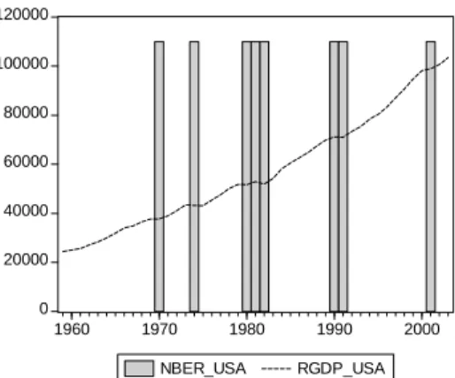
(3) Yuan-Ming Lee, Kuan-Min Wang, and T. Thanh-Binh Nguyen. 103. 2. Original CDR and Modified CDR Beaudry and Koop (1993) present the original CDR as an indicator of business cycle regime, with CDR = 0 representing expansion, and CDR > 0 indicating recession. More precisely, CDR is the gap between the maximum level of output from period s to period t and the level of output in period t :. CDR i , t = max{Yi , t − s }ts ≥0 − Yi , t ,. (1). where Yi , t is the level of output of country i in period t . The CDR is based on the trend of real output during expansions and recessions. Figure 1 illustrates the trend in US real GDP (RGDP_USA) with recessions (NBER_USA) superimposed based on data from the National Bureau of Economic Research. It is seen from the figure recessions coincide with dips in real output. Figure 1. US Real GDP Trend and Recessions 120000 100000 80000 60000 40000 20000 0 1960. 1970. 1980. NBER_USA. 1990. 2000. RGDP_USA. Notes: RGDP_USA is US real GDP (the dotted line), and NBER_USA is US recessions (the vertical bars). Data are from the National Bureau of Economic Research (http://www.nber.org/ cycle.htm).. Even if the CDR mechanism captures recessions acutely, it still suffers deficiencies. Bradley and Jansen (1997) revised part of the definition of the CDR, presenting the new CDR (NCDR) to amend the defect of non-pure recessions. Koop et al. (1996), Pesaran and Potter (1996), and Altissimo and Violant (2000) also attempted to improve the CDR. Specifically, the NCDR subdivides CDR > 0 into two states—depression and recovery—based on whether output growth is negative or positive: ⎧⎪ max{Yi , t − s }s ≥ 0 − Yi , t CDR1i , t = ⎨ 0 ⎪⎩. if Δ Yt < 0 if Δ Yt ≥ 0. (2).

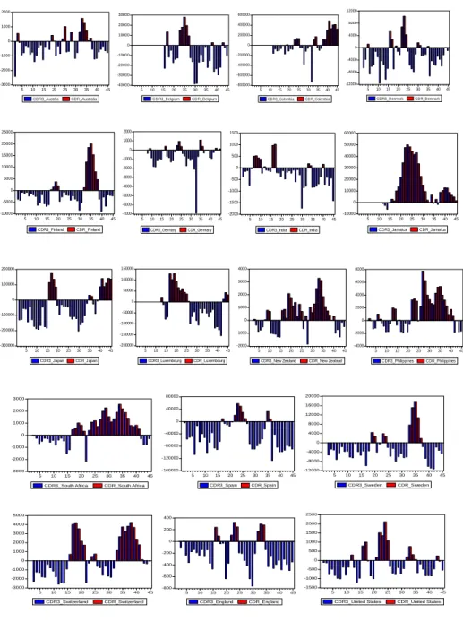
(4) 104. International Journal of Business and Economics ⎪⎧ max{Yi , t − s }s ≥ 0 − Yi , t CDR 2 i , t = ⎨ 0 ⎪⎩. if Δ Yt ≥ 0. (3). if Δ Yt < 0.. Unfortunately, threshold models with CDR or NCDR as the threshold variable often cannot be estimated since there are insufficient observations in a single regime for many countries. Additionally, the criteria determining the performance regime are exogenous, further limiting the explanatory power of the model. To overcome these limitations, we first consider a framework with states of both recession and expansion. This modification enlarges the range of the index since it is no longer truncated at zero. The modified indicator is therefore no longer restricted to recession period information and can be considered for more general datasets. The resulting CDR, denoted CDR3, represents the difference between the maximum level of output from period s to period t − 1 and the level of output in period t :. CDR 3 i , t = max{Yi , t − s }ts >0 − Yi , t ,. (4). where Yi , t indicates the level of output in period t . The CDR3 maintains the original interpretation during expansions as well as other characteristics. Beaudry and Koop (1993) showed that the CDR can be employed as a proxy variable for the business cycle. The MCDR slightly modifies the original CDR but retains the key characteristics of the CDR, and can also be used as a proxy variable. (Appendix C.) The only difference between CDR3 and CDR is whether or not output in period t is considered in the set being maximized. Figures 2 and 3 present the CDR and CDR3 for the US and for selected countries, with threshold values estimated endogenously. Figure 2. US Recessions and Expansions Defined by CDR and CDR3 2500 2000 1500 1000 500 0 -500 -1000 -1500 1960. 1970. 1980. CDR_USA. 1990. 2000. CDR3_USA. Notes: Light grey bars exhibit US recessions defined by CDR and dark grey bars display US recessions and expansions defined by CDR3..

(5) 105. Yuan-Ming Lee, Kuan-Min Wang, and T. Thanh-Binh Nguyen Figure 3. CDR and CDR3 Bar Charts for Selected Countries 12000. 2000. 1000. 30000. 600000. 20000. 400000. 8000. 10000. 200000. 4000. 0. 0. -10000. -200000. -20000. -400000. -30000. -600000. -40000. -800000. 0. -1000. 0 -4000. -2000. -3000 5. 10. 15. 20. 25. CDR3_Austrlia. 30. 35. 40. 45. 5. 10. CDR_Australia. 15. 20. 25. 30. CDR3_Belgium. 35. 40. 45. 10. 15. 20. 25. 30. CDR3_Colombia. 1000. 20000. 5. CDR_Belgium. 2000. 25000. -8000 -12000 35. 40. 5. 45. 10. 15. 20. 25. 30. CDR3_Denmark. CDR_Colombia. 1500. 60000. 1000. 50000. 500. 40000. 35. 40. 45. CDR_Denmark. 0 15000. -1000. 10000. -2000. 0. 30000. 5000. -3000. -500. 20000. -1000. 10000. -4000. 0. -5000 -5000 -10000 5. 10. 15. 20. 25. CDR3_Finland. 30. 35. 40. -6000. -1500. 0. -7000. -2000. -10000. 45. 5. 10. CDR_Finland. 15. 20. 25. CDR3_Germany. 200000. 30. 35. 40. 45. 5. 10. CDR_Germany. 15. 20. 25. CDR3_India. 30. 35. 40. 5. 45. 15. 20. 25. 30. CDR3_Jamaica. 150000. 4000. 8000. 100000. 3000. 6000. 2000. 4000. 1000. 2000. 100000. 10. CDR_India. 35. 40. 45. CDR_Jamaica. 50000 0. 0 -50000. -100000. 0. 0. -1000. -2000. -100000 -200000. -150000 -200000. -300000 5. 10. 15. 20. 25. CDR3_Japan. 30. 35. 40. -2000. 5. 45. 10. 15. 20. 25. CDR3_Luxembourg. CDR_Japan. 30. 35. 40. -4000. 45. 5. CDR_Luxembourg. 10. 15. 20. CDR3_New Zealand. 35. 40. 45. 5. 10. 15. 20. 25. CDR3_Philippines. 30. 35. 12000 1000. 0. 0. -40000. -1000. -80000. -2000. -120000. 8000 4000 0 -4000 -8000 -12000. -160000. -3000 5. 10. 15. 20. 25. CDR3_South Africa. 30. 35. 40. 5. 45. 10. 15. 20. 25. CDR3_Spain. CDR_South Africa. 5000. 30. 35. 40. 5. 45. 10. 15. 20. 25. CDR3_Sweden. CDR_Spain. 30. 35. 40. 45. CDR_Sweden. 2500. 400. 2000. 4000 200. 1500. 3000 2000. 0. 1000. 1000. -200. 500 0. 0 -400. -500. -1000 -600. -2000 -3000. -1000 -1500. -800. 5. 10. 15. 20. CDR3_Switzerland. 25. 30. 35. 40. CDR_Switzerland. 45. 5. 10. 15. 20. CDR3_England. 25. 30. 35. 40. CDR_England. 45. 5. 10. 15. 20. CDR3_United States. 25. 30. 35. 40. CDR_Philippines. 16000. 40000. 2000. 30. CDR_New Zealand. 20000. 80000. 3000. 25. 40. 45. CDR_United States. 45.

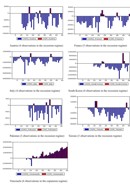
(6) 106. International Journal of Business and Economics. Figure 3 (continued). CDR and CDR3 Bar Charts for Countries with Few Recession Periods 5000. 4000 2000. 0 0. -5000. -2000 -4000. -10000 -6000. -15000. -8000. 5. 10. 15. 20. 25. CDR3_Austria. 30. 35. 40. 45. 5. 10. CDR_Austria. 15. 20. 25. CDR3_France. Austria (4 observations in the recession regime). 30. 35. 40. 45. CDR_France. France (5 observations in the recession regime). 1000000. 1200000 800000. 0. 400000. -1000000. 0 -400000. -2000000. -800000. -3000000 -1200000. -4000000. -1600000. 5. 10. 15. 20. 25. CDR3_Italy. 30. 35. 40. 45. 5. CDR_Italy. 10. 15. 20. 25. CDR3_South Korea. Italy (4 observations in the recession regime). 30. 35. 40. 45. CDR_South Korea. South Korea (4 observations in the recession regime) 20000. 400. 10000 0. 0 -400. -10000. -800. -20000. -30000. -1200 5. 10. 15. 20. 25. CDR3_Pakistan. 30. 35. 40. 5. 45. 10. 15. 20. CDR3_Taiwan. CDR_Pakistan. Pakistan (3 observations in the recession regime). 25. 30. 35. 40. 45. CDR_Taiwan. Taiwan (3 observations in the recession regime). 3000000. 2000000. 1000000. 0. -1000000. -2000000 5. 10. 15. 20. CDR3_Venezuela. 25. 30. 35. 40. 45. CDR_Venezuela. Venezuela (4 observations in the expansion regime). The proposed MCDR is basically the same as the CDR3. The only difference is that it is rescaled to avoid possible confusion caused by the opposite sign between CDR3 values and business cycle regimes and to normalize its values:.

(7) Yuan-Ming Lee, Kuan-Min Wang, and T. Thanh-Binh Nguyen − CDR 3 i , t. MCDR it =. ∑ (CDR 3. i,t. − μ CDR 3 ) 2 / N i − 1. ,. 107 (5). where μ CDR 3 is the mean of CDR3 and N i is the number of observations for country i . Thus positive MCDR values correspond to expansion regimes and negative values to recession regimes. Since the MCDR quantifies both expansionary and recessionary regimes, it is directly applicable in TAR and TVAR models for a broad range of country datasets. 3. Empirical Model and Results 3.1 Threshold Model Framework In this section, the MCDR is used as a proxy threshold variable for economic performance in a threshold model to analyze the interaction between stock returns and economic growth. To control for possible misspecification bias if other relevant variables are omitted, several macroeconomic variables and exogenous variables are included following King and Levien (1993) and Huang and Yang (2004). The bivariate VAR model of stock returns and economic growth rates is: p. p. 5. yt = α10 + ∑ α1i yt − i + ∑ β1i Rt − i + ∑ θ1 jV j , t −1 + ε t i =1. i =1. j =1. p. p. 5. i =1. i =1. j =1. Rt = α 20 + ∑ α 2i yt −i + ∑ β 2i Rt − i + ∑ θ 2 jV j , t −1 + μ t ,. (6). where yt is the economic growth rate, Rt is the stock return, α i and β i are parameters, ε t and μ t are error terms, and V j , t −1 is an exogenous variable with lag length 1. Then the threshold VAR model is: Ζ t = ( A1 +Φ 1 Ζ t −i ) I (qt − d > γ ) + ( A2 + Φ 2 ,i Ζ t −i )(1 − I (qt − d > γ )) + ε. (7). where: ⎡α 11 ...α 1 p ⎤ ⎡α 21 ...α 2 p ⎤ ⎡α ⎤ ⎡α ⎤ ⎡y ⎤ Ζ t = ⎢ t ⎥ , Α 1 = ⎢ 10 ⎥ , A 2 = ⎢ 20 ⎥ , Φ 1 = ⎢ ⎥ , Φ 2 = ⎢ β ...β ⎥ β ... β R β β ⎣ 20 ⎦ 2×1 ⎣ 10 ⎦ 2×1 ⎣ t ⎦ 2×1 ⎣ 11 1 p ⎦ 2× p ⎣ 21 2 p ⎦ 2× p. with p the lag length, qt−d the threshold variable, d the delay parameter, γ the threshold value, ε = (ε 1* ε 2* )' the error term with E (ε t | Ωt −1 ) ~ iid(0, σ 2 ) , Ω t −1 the information set of the previous period, and I (⋅) the standard indicator function. 3.2 Data Description and Unit Root Tests We consider seven variables to demonstrate the performance of MCDR using data from selected countries:.

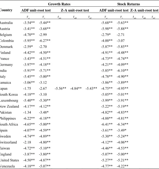
(8) 108. International Journal of Business and Economics. (1) LSR: the logarithm of stock index. (2) LYG: the growth rate of real per capita GDP. LYG is calculated as the first differential of the ratio of GDP to the GDP deflator and total population. This adjustment controls for heterogeneity in nominal GDP and in populations across countries. (3) GOV: how much government consumption influences the whole economy, measured as the ratio of government consumption to GDP. (4) INV: a proxy variable for capital stock, measured as the ratio of the gross fixed capital formation to GDP. It is one of the major factors in the output function. (5) LPG: a proxy variable for labor, measured as the logarithm of the population differential. It is the other major factor in the output function. (6) TRD: a proxy for economic openness, measured as the ratio of the sum of imports and exports to GDP. (7) PI: the logarithm of the consumer price index (CPI). A high inflation rate has a negative impact on the economic growth and stock returns. Variables (1) and (2) represent stock returns and economic growth rates; these are the main variables of interest. Variables (3) to (7) are exogenous and are selected based on the empirical models of Bekaert et al. (2001), King and Levien (1993), Sarel (1996), and Hung (2001). Exogeneity of these variables was justified based on impulse response analysis of all seven variables in panel-VAR (available upon request). To estimate the bivariate model, the number of observations in each regime must be taken into consideration. Observations within each regime do not allow considering the nonlinearity in the model. Our analysis is based on annual data, like Fama (1990) and Mauro (2003), to avoid exogenous short-run noise that may bias empirical results. We consider 25 countries from 1960 to 2003. Appendices A and B present detailed information on countries, data codes, and data sources. According to the nonlinearity test of Tsay (1998), the MCDR with delay parameter d = 1, 2,3 is adopted as the threshold variable in the model with 1 to 3 lag lengths 1 to 3 for the endogenous variables. The models are built based on a two-regime TVAR model using the equation (7) as the basic model. An economy belongs to regime 1 when the threshold variable is greater than the threshold value, and belongs to regime 2 otherwise. The lag lengths of exogenous variables and the delay of the threshold variable are given in Table 2. As suggested by Weise (1999), the smallest determinant value of the residual covariance matrix is used to select the optimal threshold value. The use of nonstationary data can lead to spurious results. Therefore, we use the augmented Dickey-Fuller (ADF) test to test for unit roots of variables (Granger and Newbold, 1974). Further, due to the length of the study period, there might be structural breaks in the series. Therefore, we use the test developed by Bai and Perron (2003) to identify the existence of structural breaks. The unit root test of Zivot and Andrew (1992) is applied to series that have a single structural break to check for their unit roots. To test for unit roots in series that have more than one structural break, the structural breaks are first added to the equation of traditional.

(9) 109. Yuan-Ming Lee, Kuan-Min Wang, and T. Thanh-Binh Nguyen. ADF to construct modified ADF tests for series with multiple structural breaks. The critical value used to determine stationarity is selected via bootstrapping. Table 1 reports the results of unit root tests. Most series have multi-structural breaks that are tested for unit-root by the ADF test with structural breaks. This approach rejects obviously the null hypothesis of nonstationary in all series, providing evidence of stationarity for all variables. Table 1. Unit Root Tests Growth Rates Country. ADF unit-root test. τμ. ττ. Stock Returns. Z-A unit-root test tαÂ. tαˆB. tαˆC. ADF unit-root test Z-A unit-root test. τμ. ττ. Australia. -3.54**. -5.44**. -5.68**. -5.63**. Austria. -3.41**. -3.68**. -5.98**. -5.88**. Belgium. -4.70**. -2.99. -2.79*. -2.71. Colombia. -5.95**. -6.27**. -4.00**. -3.07. Denmark. -2.59*. -2.70. -5.87**. -5.85**. Finland. -4.42**. -4.50**. -4.91**. -4.48**. France. -3.43**. -4.51**. -4.73**. -4.74**. Germany. -3.97**. -4.18**. -4.21**. -4.09**. India. -5.91**. -5.71**. -5.85**. -6.10**. Italy. -5.45**. -5.00**. -4.78**. -4.90**. Jamaica. -3.06**. -3.12. -3.86**. -3.89**. Japan. -1.75. -2.67. South Korea. -4.18**. Luxembourg New Zealand. -5.56**. -4.84**. -5.43**. -4.75**. -4.95**. -3.10. -5.05**. -5.01**. -5.40**. -5.30**. -3.99**. -3.91**. -4.17**. -4.12**. -5.22**. -5.19**. Pakistan. -1.34. -3.48*. -4.82**. -4.83**. Philippines. -6.22**. -6.18**. -4.88**. -4.81**. South Africa. -4.65**. -5.00**. -6.41**. -6.34**. Spain. -4.07**. -4.59**. -3.61**. -3.49*. Sweden. -4.74**. -4.89**. -5.30**. -5.24**. Switzerland. -2.18. -4.80**. -4.12**. -4.06**. Taiwan. -4.72**. -5.10**. -4.46**. -4.53**. England. -3.87**. -3.80**. -5.07**. -5.00**. United States. -4.50**. -4.87**. -5.27**. -5.21**. tαÂ. tαˆB. tαˆC. Venezuela -4.18** -5.07** -4.77** -4.22** Notes: τ μ denotes the constant and τ τ denotes the constant and time trend in the unit root equation. The Z-A unit-root test is based on Zivot and Andrews (1992) and allows for series with one break, using the Akaike information criterion to select for optimal lag. The 5% and 10% threshold limits for models A, B, and C are (−4.80, −4.58), (−4.42, −4.11), and (−5.08, −4.82). Statistics ending with “s” correspond to variables with more than one structural break and are based on the multiple-break ADF unit root test with threshold limits obtained via bootstrapping. * and ** denote significance at the 10% and 5% levels..

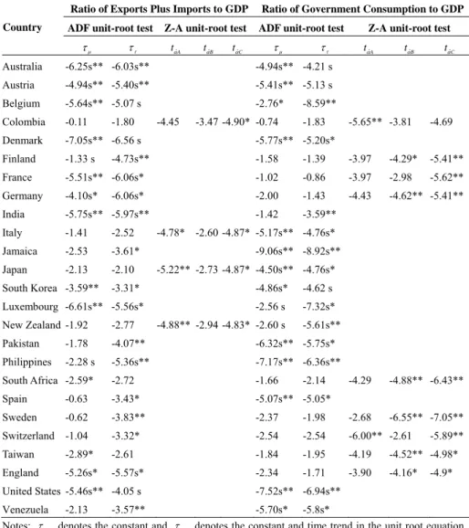
(10) 110. International Journal of Business and Economics Table 1 (continued). Unit Root Tests Ratio of Exports Plus Imports to GDP. Ratio of Government Consumption to GDP. Country. ADF unit-root test. ADF unit-root test. Australia. -6.25s** -6.03s**. -4.94s** -4.21 s. Austria. -4.94s** -5.40s**. -5.41s** -5.13 s. Belgium. -5.64s** -5.07 s. Colombia. -0.11. Denmark. -7.05s** -6.56 s. Finland. -1.33 s. France. -5.51s** -6.06s*. τμ. ττ. -1.80 -4.73s**. Germany. -4.10s*. India. -5.75s** -5.97s**. -6.06s*. Italy. -1.41. -2.52. Jamaica. -2.53. -3.61*. Japan. -2.13. -2.10. South Korea -3.59**. -3.31*. Luxembourg -6.61s** -5.56s* New Zealand -1.92. -2.77. Z-A unit-root test tαÂ. tαˆB. tαˆC. τμ. -2.76* -4.45. -3.47 -4.90* -0.74. ττ. Z-A unit-root test tαÂ. tαˆB. tαˆC. -5.65** -3.81. -4.69. -8.59** -1.83. -5.77s** -5.20s* -1.58. -1.39. -3.97. -4.29*. -5.41**. -1.02. -0.86. -3.97. -2.98. -5.62**. -2.00. -1.43. -4.43. -4.62** -5.41**. -1.42. -3.59**. -4.29. -4.88** -6.43**. -2.68. -6.55** -7.05**. -4.78* -2.60 -4.87* -5.17s** -4.76s* -9.06s** -8.92s** -5.22** -2.73 -4.87* -4.50s** -4.76s* -4.86s*. -4.62 s. -2.56 s. -7.32s*. -4.88** -2.94 -4.83* -2.60 s. -5.61s**. Pakistan. -1.78. -4.07**. -6.32s** -5.75s*. Philippines. -2.28 s. -5.36s**. -7.17s** -6.36s**. South Africa -2.59*. -2.72. -1.66. Spain. -0.63. -3.43*. -5.07s** -5.05*. -2.14. Sweden. -0.62. -3.83**. -2.37. -1.98. Switzerland -1.04. -3.32*. -2.54. -2.54. -6.00** -2.61. Taiwan. -2.89*. -2.61. -1.84. -1.95. -4.19. -4.52** -4.98*. England. -5.26s*. -5.57s*. -2.34. -1.71. -3.90. -4.16*. United States -5.46s** -4.05 s. -5.89** -4.9*. -7.52s** -6.94s**. Venezuela -2.13 -3.57** -5.70s* -5.8s* Notes: τ μ denotes the constant and τ τ denotes the constant and time trend in the unit root equation. The Z-A unit-root test is based on Zivot and Andrews (1992) and allows for series with one break, using the Akaike information criterion to select for optimal lag. The 5% and 10% threshold limits for models A, B, and C are (−4.80, −4.58), (−4.42, −4.11), and (−5.08, −4.82). Statistics ending with “s” correspond to variables with more than one structural break and are based on the multiple-break ADF unit root test with threshold limits obtained via bootstrapping. * and ** denote significance at the 10% and 5% levels..

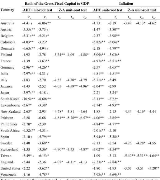
(11) 111. Yuan-Ming Lee, Kuan-Min Wang, and T. Thanh-Binh Nguyen Table 1 (continued). Unit Root Tests Ratio of the Gross Fixed Capital to GDP Country. ADF unit-root test. Australia. -4.41 s. Austria Belgium. τμ. ττ. Z-A unit-root test. Inflation ADF unit-root test. ττ. tαÂ. -1.73. -2.19. -3.49. -4.13* -4.62. -5.55s** -3.73 s. -1.47. -3.80**. -5.31s** -5.21s*. -2.37. -3.98**. Colombia. -4.03**. -5.82s** -5.06s*. Denmark. -6.63s** -4.94 s. Finland. -1.92. -2.78. France. -1.39. -3.63**. Germany. -2.96**. -4.26**. India. -7.97s** -4.31 s. Italy. -1.83. -2.70. -4.55. -4.30* -4.79. Jamaica. -1.43. -2.52. -4.05. -4.59** -4.96* -3.04**. Japan. -5.97s** -4.18 s. -4.44. -4.16* -4.44. -4.26. -4.28* -4.55. tαÂ. tαˆB. tαˆC. -6.06s**. -3.23*. τμ. Z-A unit-root test. -2.18 -5.34** -4.09. -4.79**. -4.97s** -5.51s** -2.57. -3.65**. -4.81**. -4.81**. -5.71s** -5.49 -2.21. -2.99 -3.24*. -3.13**. -3.22*. Luxembourg -2.67*. -3.38*. -2.74*. -4.93**. New Zealand -2.63*. -2.93. -4.78* -3.81. -1.88. -2.13. -4.64. Pakistan. -2.28. -0.68. -4.81** -5.78** -8.57** -4.06**. -3.85**. Philippines. -2.70*. -2.39. -4.84**. -4.77**. South Africa -6.52s** -4.31 s. -7.01s** -5.10. Spain. -3.10 s. -5.79s**. -5.94s** -5.38s*. Sweden. -1.40. -3.68**. -2.13. -1.33. -3.36*. Taiwan. -3.49* s. -6.15s*. England. -2.44. -2.36. United States -2.22. -3.62**. tαˆC. -4.88* -5.09s** -5.03s*. South Korea -10.5s** -8.60s**. Switzerland. tαˆB. -4.90** -3.75. -4.87* -3.02** -1.09. -4.07* -4.11* -4.13. -2.54 -3.54** -3.13. -5.40** -5.31** -4.64**. -7.23s** -7.84s** -1.80. -1.93. -3.07. -3.51. -5.20**. Venezuela -1.16 -4.78** -5.98s** -6.69s** Notes: τ μ denotes the constant and τ τ denotes the constant and time trend in the unit root equation. The Z-A unit-root test is based on Zivot and Andrews (1992) and allows for series with one break, using the Akaike information criterion to select for optimal lag. The 5% and 10% threshold limits for models A, B, and C are (−4.80, −4.58), (−4.42, −4.11), and (−5.08, −4.82). Statistics ending with “s” correspond to variables with more than one structural break and are based on the multiple-break ADF unit root test with threshold limits obtained via bootstrapping. * and ** denote significance at the 10% and 5% levels..

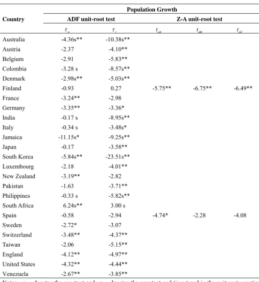
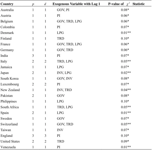
(12) 112. International Journal of Business and Economics Table 1 (continued). Unit Root Tests Population Growth. Country. ADF unit-root test. τμ Australia. -4.36s**. Austria. -2.37. ττ. -2.91. -5.83**. -3.28 s. -8.57s**. Denmark. -2.98s**. -5.03s**. Finland. -0.93. France. -3.24**. -2.98. Germany. -3.35**. -3.36*. India. -0.17 s. -8.95s**. Italy. -0.34 s. -3.48s*. -11.15s*. -9.25s**. 0.27. Japan. -0.17. South Korea. -5.84s**. Luxembourg. -2.18. -4.01**. New Zealand. -3.19**. -2.82. Pakistan. -1.63. -3.71**. Philippines. -0.33 s. -5.82s**. 6.24s**. tαˆB. tαˆC. -4.10**. Colombia. South Africa. tαÂ. -10.38s**. Belgium. Jamaica. Z-A unit-root test. -5.75**. -6.75**. -6.49**. -4.74*. -2.28. -4.08. -3.58** -23.51s**. 3.00 s. Spain. -0.58. -2.94. Sweden. -2.72*. -3.07. Switzerland. -3.48**. -4.37**. Taiwan. -2.06. -5.15**. England. -4.12**. -4.97**. United States. -4.32**. -4.44**. Venezuela -2.67** -3.85** Notes: τ μ denotes the constant and τ τ denotes the constant and time trend in the unit root equation. The Z-A unit-root test is based on Zivot and Andrews (1992) and allows for series with one break, using the Akaike information criterion to select for optimal lag. The 5% and 10% threshold limits for models A, B, and C are (−4.80, −4.58), (−4.42, −4.11), and (−5.08, −4.82). Statistics ending with “s” correspond to variables with more than one structural break and are based on the multiple-break ADF unit root test with threshold limits obtained via bootstrapping. * and ** denote significance at the 10% and 5% levels.. 3.3 Empirical Results and Analysis Our analysis is based on time series data of 25 countries, including OECD and Asian emerging economies. The nonlinearity test is applied to examine if the model the threshold model using the MCDR as its threshold variable is appropriate. This approach allows us to verify whether the relationship between stock returns and economic growth varies with the economic regimes and to further understand the performance of the MCDR as the threshold variable. Based on the results in Table 2,.

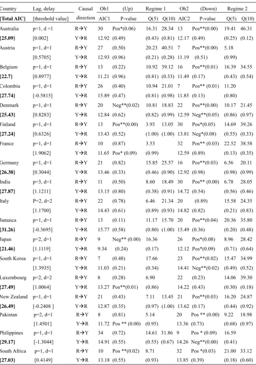
(13) Yuan-Ming Lee, Kuan-Min Wang, and T. Thanh-Binh Nguyen. 113. we conclude that it is reasonable to use the MCDR as a threshold variable and to build the TVAR model. Table 2. Nonlinearity Tests with Threshold Variable MCDR Country. p. d. Exogenous Variable with Lag 1. P-value of χ 2 Statistic. Australia. 1. 1. GOV, PI. 0.08*. Austria. 1. 1. PI. 0.06*. Belgium. 1. 1. GOV, TRD, LPG. 0.06*. Colombia. 1. 1. PI. 0.07*. Denmark. 1. 1. LPG. 0.01**. Finland. 1. 1. TRD. 0.10*. France. 1. 1. GOV, TRD, LPG. 0.06*. Germany. 1. 1. GOV, TRD. 0.06*. India. 3. 1. PI. 0.07*. Italy. 2. 2. TRD, LPG. 0.05**. Jamaica. 1. 1. LPG. 0.07*. Japan. 2. 1. INV, LPG. 0.02**. South Korea. 1. 1. GOV, INV. 0.08*. Luxembourg. 2. 2. PI. 0.07*. New Zealand. 1. 1. INV, TRD. 0.04**. Pakistan. 2. 1. GOV. 0.08*. Philippines. 1. 1. LPG. 0.10*. South Africa. 1. 1. TRD, LPG. 0.05**. Spain. 2. 1. LPG. 0.01**. Sweden. 1. 1. GOV. 0.07*. Switzerland. 1. 1. GOV, TRD. 0.05**. Taiwan. 1. 1. INV. 0.07*. England. 3. 3. PI. 0.10*. United States. 2. 2. TRD. 0.09*. Venezuela 1 1 PI 0.01** Notes: All variables are exogenous except LYG and LSR. In the vector model, these variables have lag 1. p is the lag length of the endogenous variables. d is the delay parameter of threshold variable. P-values are for χ 2 statistics, * and ** flagging p-values smaller than 10% and 5%.. Table 3 reports estimation results of the TVAR model, which exhibits causality between stock returns and economic growth rates. During expansion (regime 1), there obviously exists a causal relationship between lagged stock returns and current growth rates in 6 countries: Australia, Finland, and South Africa with positive relationships and Denmark, Japan, and Taiwan with negative relationships. There is insignificant evidence of causal relationships in the remaining 19 countries..

(14) 114. International Journal of Business and Economics Table 3. TVAR Analysis of Business Cycles with Threshold Variable MCDR Causal. Country. Lag, delay. {Total AIC}. [threshold value]. direction AIC1. Ob1. Australia. p=1, d =1. RÆY. {25.09}. [0.002]. YÆR. 12.92 (0.49). (0.43) (0.81) 12.17 (0.49). Austria. p=1, d=1. RÆY. 27. 20.23 40.51 7. [0.5705]. YÆR. 12.93 (0.96). (0.21) (0.28) 11.19 10.92 39.12 16. 30. (Up) P-value Pos*(0.06). (0.50). Belgium. p=1, d=1. RÆY. 13. {22.7}. [0.8977]. YÆR. 11.21 (0.96). (0.22). (0.40). Regime 1. Ob2. (Down). Regime 2. Q(5) Q(10) AIC2. P-value. Q(5) Q(10). 16.31 28.34 13. Pos**(0.00). Pos**(0.00) (0.51) Pos**(0.01). (0.81) (0.33) 11.49 (0.17). (0.25) (0.12) 5.18 (0.99) 16.39 34.55 (0.43) (0.54). Colombia. p=1, d=1. RÆY. 26. {27.74}. [-0.5815]. YÆR. 15.89 (0.47). (0.81) (0.98) 11.85 (0.13). (0.80). Denmark. p=1, d=1. RÆY. 20. 10.81 18.83 22. 10.17 21.45. {25.43}. [0.8283]. YÆR. 12.84 (0.62). (0.82) (0.99) 12.59 Neg**(0.05) (0.86) (0.97). Finland. p=1, d=1. RÆY. 13. 3.93. {27.24}. [0.6326]. YÆR. France. p=1, d=1. RÆY. Neg**(0.02). Pos**(0.00). 10.94 21.01 7. 19.41 46.31. Pos**(0.00). Pos*(0.05). 14.69 39.26. 13.43 (0.52). (1.00) (1.00) 13.81 Neg*(0.08). (0.55) (0.33). 10. 3.53. 32. 12.59 (0.89). (0.87). 13.05 30. Pos** (0.01) 11.20. Pos** (0.03) 22.52 38.58. [1.9062]. YÆR. 11.65 Pos* (0.09). (0.99). Germany. p=1, d=1. RÆY. 21. 15.85 25.57 16. {26.38}. [0.3044]. YÆR. 13.46 (0.33). (0.46) (0.90) 12.92 (0.98). India. p=3, d=1. RÆY. 11. 8.60. {27.87}. [1.1211]. YÆR. 13.15 (0.80). (0.38) (0.91) 14.72 (0.54). Italy. P=2, d=2. RÆY. 22. 6.46. [1.1700]. YÆR. 14.43 (0.61). Jamaica. p=1, d=1. RÆY. 13. {31.26}. [-0.3695]. YÆR. 15.77 (0.58). Japan. p=2, d=1. RÆY. 9. {21.46}. [1.1119]. YÆR. 9.34. South Korea. (0.82). (0.50). (0.78). (0.11). 21.34 20. 11.17 15.70 20. (0.89). Pos**(0.04). (0.80) (1.00) 15.49 (0.36) 26. (0.13) (0.35) 6.56. Pos*(0.08). 20.11. (0.98) (0.99). Pos** (0.00) 6.78. (0.89) (0.93) 14.82 (0.82). Neg** (0.00) 16.36 (0.24). 18.49 30. Pos**(0.03). 28.05. (0.56) (0.46) 15.58 24.35 (0.21) (0.83) 20.36 35.80 (0.20) (0.48) 8.96. 28.42. (0.17). 12.12 Pos*(0.09). (0.71) (0.64) 15.47 34.99. p=1, d=1. RÆY. 7. (0.48). 17.66. 23. [1.3935]. YÆR. 11.03 (0.21). (0.34). 14.41 Neg**(0.02) (0.49) (0.52). Luxembourg. p=2, d=2. RÆY. 8. 6.90. 22. (0.28). Pos**(0.02). (0.23). 14.06 39.30. 14.22 (0.43). (0.30) (0.18). {27.49}. [1.0064]. YÆR. 13.27 Pos**(0.01). (0.86). New Zealand. p=1, d=1. RÆY. 21. 7.11. {26.49}. [-0.2408 ]. YÆR. 12.87 (0.35). (0.97) (1.00) 13.62 (0.17) 5.14. (0.43). p=2, d=1. RÆY. 8. [1.4501]. YÆR. 11.72 Pos ** (0.00) (0.95). Philippines. p=1, d=1. RÆY. 34. {29.17}. [-1.3044]. YÆR. 14.91 (0.55). Pakistan. (0.81) (0.72). South Africa. p=1, d=1. RÆY. 10. {27.03}. [0.4149]. YÆR. 13.18 (0.55). Pos **(0.02). 13.45 21 20. Pos**(0.03). Pos ** (0.00) 9.22. 13.36 (0.73). 14.61 31.86 9. 16.20 24.87 (0.44) (0.92). Pos * (0.09). 16.59. (0.55) (0.67) 14.26 Neg**(0.00). (0.41). 8.71. 32. (0.93). 13.85 (0.39). Pos *(0.03). 18.98. (0.68) (0.97). 21.00 33.12 (0.18) (0.60).

(15) 115. Yuan-Ming Lee, Kuan-Min Wang, and T. Thanh-Binh Nguyen Table 3 (continued). TVAR Analysis of Business Cycles with Threshold Variable MCDR Causal. Country. Lag, delay. {Total AIC}. [threshold value]. direction AIC1. Spain. p=2, d=1. RÆY. {26.13}. [1.0812]. YÆR. 12.58 Neg**(0.05). (0.37) (0.90) 13.55 (0.40). Sweden. p=1, d=1. RÆY. 7. 9.09. {25.36}. [1.0647]. YÆR. 11.93 (0.69). (0.91). Switzerland. p=1, d=1. RÆY. 13. 9.63. {25.57}. [0.5649]. YÆR. 12.61 (0.36). Taiwan. Ob1. 23. (Up) P-value (0.16). (0.14). (0.57). Regime 1. Ob2. (Down). Regime 2. Q(5) Q(10) AIC2. P-value. Q(5) Q(10). 13.02 22.10 19. 35. Pos **(0.01). Pos **(0.00). (0.88) (0.99) 12.96 (0.19). Neg** (0.03) 12.94 32.48 23. (0.34) (0.63). Pos * *(0.05) 14.59 36.27. 13.43 (0.47) 19.54 29. 13.39 28.75. (0.55) (0.46) 7.30. 20.59. (0.97) (0.98). p=1, d=1. RÆY. 12. (0.92). 17.02 30.12. [1.5559]. YÆR. 14.65 (0.87). (0.68) (0.64) 14.61 (0.11). (0.38) (0.74). England. p=3, d=3. RÆY. 12. 6.42. {23.01}. [1.3565]. YÆR. 11.18 (0.72). (0.60) (0.94) 11.83 (0.42). United States. p=2, d=2. RÆY. 32. 4.59. {22.47}. [-0.2586]. YÆR. 12.73 (0.69). (0.97) (0.97) 9.74. Neg** (0.02) (0.94). Venezuela. p=1, d=1. RÆY. 12. 17.79 34.80 21. (0.68). [-0.47156]. YÆR. 16.18 (0.80). (0.15). (0.33). (0.43). 17.49 28. 18.25 10. Pos **(0.03). 9.62. 28.36. (0.29) (0.44). Pos ** (0.00) 5.38. (0.34) (0.53) 17.67 (0.52). 18.55 41.13 0.29. (0.26). Notes: All exogenous variables have lag 1 except the constant. p denotes the lag of endogenous variables, and d denotes the delay of the threshold variable. The optimal threshold value and the model selection criterion are based on the smallest determinant value of the residual covariance matrix. Ob1 and Ob2 represent the number of adjusted observations in both regime 1 and 2. RÆY indicates that the stock returns can explain economic growth, and YÆR indicates that economic growth can explain stock returns. P-values of the joint test are in parentheses, with * and ** denoting p-values smaller than 10% and 5%. Here Pos and Neg denote significant positive and negative effects. The positive or negative effect of a coefficient is determined by its sum, which is positive or negative. Q(k) is the multivariate Box-Piece/Ljung-Box χ 2 statistic used to test for serial correlation of residuals in adjusted data for k=5, 10 lag lengths. {Total AIC} presents the sum of AIC values in the two regimes.. During recessions (regime 2), 21 countries display significantly the causal relationships between lagged stock returns and current growth rates, each with positive signs. This relationship in more than 80% of the countries supports results obtained by Mauro (2003) and Henry et al. (2004). This positive relationship is observed in 3 countries (Australia, Finland, and Japan) in both regimes 1 and 2. Moreover, bidirectional causality appears in 5 countries (Denmark, Finland, Japan, Philippines and the US). However, Italy, Luxembourg, Taiwan, and Venezuela do not present causality in regime 2. In summary, in the two-regime TVAR framework, positive causality between stock returns and growth occurs primarily during recessions. However, this relation is not significant during expansions. It is noteworthy that positive causality is clearest in countries with high income. The threshold value is between 1.91 and −0.26 standard deviations in high income countries, tending toward expansion, between 0.41 and −1.30 in medium low income countries, inclining towards recession, and between 1.12 and 1.45 in low income countries, strongly favoring expansion. The higher threshold values in high and low income countries show that these economies belong to regime 1 during.

(16) 116. International Journal of Business and Economics. relatively prosperous periods. Similarly, the economy of medium low income countries belongs to regime 2 during relatively recessionary periods. Choi et al. (1999), Aylward and Glen (2000), and Mauro (2003) also find that stock returns can predict future economic activities. Domian and Louton (1997) and Henry et al. (2004) conclude that the relationship between stock returns and economic growth is significant during recessions but insignificant during expansions. These different findings may be caused by anticipation of stock returns to economic growth conditions. Since stock returns decrease during recessions and increase rapidly during recoveries, the trend behavior is evident. Beaudry and Koop (1993) and Henry et al. (2004) name this phenomenon the “bounce-back” effect. Although stock returns reflect economic growth during expansions, it is usually not significant because excessive optimism might cause the bubbles. Another explanation may be that there are numerous high-return investments; during expansions investors might shift capital to non-stock investments to hedge risk. Binswanger (2004) supports this explanation. However, the impact of short-term speculative bubbles is partially mitigated by our choice to analyze annual data. 4. Conclusion This article proposes a common-use measure of economic performance obtained by a slight modification to the standard definition of current depth of recession. The proposed measure, termed MCDR, can be used as a threshold variable in econometric threshold models of time series data. We demonstrate performance of the proposed measure in an empirical analysis of causal relationships between stock returns and economic growth for 25 countries from 1960 to 2003. Our results obtained are consistent with those in the literature (e.g., Henry et al., 2004). Specifically, we find that stock returns lead economic growth rates in most countries during recessions but that stock returns cannot predict growth during expansions. We conclude that the MCDR can be a useful proxy for business cycle regimes. The most obvious advantage of using the MCDR as the threshold variable in a threshold model is that, in contrast with the conventional definition of the CDR and alternative modifications such as the NCDR, it can be used to develop nonlinear models. There are three additional strengths of the proposed MCDR. First, the MCDR is easy to calculate. Second, the MCDR overcomes a nontrivial limitation of the standard CDR in that it can be applied to data from countries with prolonged periods of growth. Third, from a methodology perspective, the MCDR in a threshold model smoothly fits the data, extending the scope of practical applications. In particular, it allows for standard nonlinearity tests. In summary, the MCDR is directly applicable as a threshold variable in econometric threshold models and can serve as a useful variable to control for macroeconomic performance regimes..

(17) 117. Yuan-Ming Lee, Kuan-Min Wang, and T. Thanh-Binh Nguyen. Appendix A. Data Summary Country. Income. Code. Country. Income. Code. Australia. Observations 44. HI. AUS. Luxembourg. Observations 32. HI. LUX. Austria. 35. HI. AUT. New Zealand. 43. HI. NZL. Belgium. 30. HI. BEL. Pakistan. 30. LO. PAK. Colombia. 34. ML. COL. Philippines. 44. ML. PHI. Denmark. 43. HI. DEM. South Africa. 43. ML. SAF. Finland. 44. HI. FIN. Spain. 44. HI. SPN. France. 43. HI. FRA. Sweden. 43. HI. SWD. Germany. 38. HI. GEM. Switzerland. 43. HI. SWL. India. 44. LO. IND. Taiwan. 36. HI. TWN. Italy. 44. HI. ITA. England. 43. HI. UK. Jamaica. 33. ML. JAM. Japan. 37. HI. JAP. United States. 44. HI. USA. Korea 31 HI KOR Venezuela 34 ML VEN Notes: According to the World Bank’s 2003 classification of per capita income, a country belongs to the low income group (LO) if per-capita income is lower than USD 765, the medium low income group (ML) if per-capita income is between USD 766 and USD 3035, and in the high income group (HI) if per-capita income is greater than USD 3036.. Appendix B. Data Sources B-1. IMF, International Financial Statistics Database Data Description. Code. Share price index. Data Description. Code. 62. Consumer price index. 64. *L64. Imports of goods and services. 98C. *L98C. Government consumption. 91. *L91F. Gross domestic product. 99B. *L99B. Gross fixed capital formation. 93E. *L93E. GDP deflator index. 99BIR. Exports of goods and services 90C *L90C Population Notes: * denotes the data obtaining from Taiwan AREMOS/UNIX.. 99Z. *L99Z. B-2. INTLINE of AREMOS/UNIX: International Economic Statistics Database Data Description Gross domestic product Imports of goods and services Gross fixed capital. Code. Data Description. Axxxvngdp Qxxxvngdp. Exports of goods and services. Code Axxxvngsx Qxxxvngsx. Axxxvngsm Qxxxvngsm Government consumption Axxxvnttcg Qxxxvnttcg. Axxxvntfi formation Notes: xxx is the country code.. Qxxxvntfi. Consumer price index. Qxxxpsttr. Mxxxpsttr.

(18) 118. International Journal of Business and Economics. Appendix C. Additional Discussion of CDR, NCDR and CDR3/MCDR It is natural to ask why we choose not to use the NCDR. There are two answers. First, like the CDR, the NCDR takes zero values during expansions. It is observed in Figure 3 that if CDR is employed as the threshold valuable, 7 of the 25 countries have five or fewer recession periods, making estimation of the TVAR model challenging or impossible. Second, we note that MCDR can easily be divided into two components with one that matches the original CDR exactly. This deconstruction proves the preservation of the original CDR properties directly for this component. The new component, which quantifies relative performance during expansionary periods instead of truncating at zero, essentially provides the mirror image of the original CDR. It is precisely because of this extension that the MCDR utilizes additional information ignored by the original CDR and can estimate regime switching with an endogenous threshold variable. To elucidate the mathematical relationship between the CDR and the CDR3 (or MCDR) first recall the definition: CDR3t = max{Yt −s }ts>0 − Yt .. Let S = 0 in the CDR, S = 1 in the MCDR. Then the mathematical relationship between CDR3 and CDR is: CDRt = max{Yt − s }ts = 0 − Yt = max{Yt , Yt −1 , Yt − 2 + K + Y1} − Yt Yt − Yt = 0, if max{Yt , Yt −1 , Yt − 2 ,K , Y1} = Yt ⎧ CDRt = ⎨ Y − Y ⎩ t − s t > 0 if max{Yt , Yt −1 ,K , Y1} = Yt − S > Yt , s > 1, t > s CDR3t = max{Yt − s }ts =1 − Yt = max{Yt −1 , Yt − 2 + K + Y1} − Yt CDR3t = max{Yt −1 , Yt − 2 ,K , Y1} − Yt + (Yt − Yt = 0 if max{Yt , Yt −1 ,K , Y1} = Yt ) ⎧Y − Y > 0 if max{Yt , Yt −1 ,K , Y1} = Yt − s , s > 1, t > s = ⎨ t −s t ⎩ Yt − s − Yt < 0 if max{Yt , Yt −1 ,K , Y1} = Yt , s > 1, t > s + (Yt − Yt = 0 if max{Yt , Yt −1 ,K , Y1} = Yt ) CDR3t = [Yt − s − Yt < 0 if max{Yt , Yt −1 ,K , Y1} = Yt , s > 1, t > s ] + CDRt. In words, the CDR and the CDR3 differ by the given term. The difference between NCDR and CDR is not very obvious; however, this difference is considerable in identifying recessionary periods. If the CDR identifies a recession, the NCDR differentiates between a depression and recovery within the recession based on whether output growth is negative or positive. Both measures are truncated at zero for expansions. Therefore, the difference between the NCDR and the CDR is limited to identification of economic performance regimes within recessions. As noted in the text, the CDR3 and the MCDR differ only in terms of a rescaling. The comparison standard used for the threshold variables is the value of the.

(19) 119. Yuan-Ming Lee, Kuan-Min Wang, and T. Thanh-Binh Nguyen. minimum of AIC sum. Tables 3 and D1 present the performance of models of 18 counties using threshold variable MCDR and CDR in terms of the minimum AIC. We find that except for Austria, the threshold values selected by both CDR and MCDR are almost the same for Jamaica and Spain, the threshold values selected by CDR are superior, and the threshold values selected by MCDR are better for the other 15 countries. To evaluate the performance according to the causality between stock return and economic growth, we observe that the causalities in both regimes are similar. These results are evident in Table D1. In other words, the positive relationship between stock return and economic growth presents the same relationship in both regimes. Table 3 shows that recessions (regime 2) tend to detect the causality between stock returns and economic growth; therefore, asymmetric causality should exist. The results found in the 18 sample countries and in the 25 sample countries are similar, supporting the robustness of empirical results. Similarly, again based on performance in terms of the minimum AIC, we find that the NCDR threshold variable underperforms the MCDR. These results are evident in Table 3 and Table D2 with 6 sample countries. Table D1. TVAR Analysis of the Business Cycle with Threshold Variable CDR Country. Lag, delay. Causal. Ob1. ( CDR =0 ) Regime 1. {Total AIC} [threshold value] direction AIC1 P-value Australia. p=1, d =1. RÆY. 30. Pos*(0.06). {25.09}. [0.00]. YÆR. 12.92. (0.74). Austria. p=1, d=1. RÆY. [0.00]. YÆR. p=1, d=1. RÆY. 21. Pos**(0.02). Belgium {24.37} Colombia. Ob2. 16.31 28.34. 13. (0.43) (0.81) 12.17. (0.25) (0.12). 8. (0.72). 21.22 (0.17). [0.00]. YÆR. 12.26. (0.86). (0.94) (0.48) 12.11. (0.69). p=1, d=1. RÆY. 20. (1.00). 14.64 29.61. (0.86). 8.34 32.99. (0.72). (0.94) (0.61). 13. RÆY. 31. (0.29). 17.73 31.66. {25.63}. [0.00]. YÆR. 13.17. (0.96). (0.34) (0.68) 12.46. Finland. p=1, d=1. RÆY. 32. Pos**(0.04). {29.40}. [0.00]. YÆR. 14.59. (0.24). France. p=1, d=1. RÆY. [0.00]. YÆR. Germany. p=1, d=1. RÆY. 28. 15.42 Pos**(0.01) (0.55) (0.77) 16.38. [0.00]. YÆR. 13.98. (0.19). p=3, d=1. RÆY. 31. Pos**(0.01). {29.2}. [0.00]. YÆR. 14.85. (0.59). P=2, d=2. RÆY. [0.00]. YÆR. 5.87 14.57. 11 11. Pos**(0.00). 7.34 21.11. (0.33). (0.97) (0.98). (0.58). 7.80. 7.93. (0.99) (1.00) 14.81 Neg**(0.01) (0.95) (1.00) 5. NA. 9. Pos*(0.08). 3.78. (0.41). (1.00). NA (0.20). India Italy. (0.49) NA. 8.38 35.70. YÆR. {26.86}. Q(10). Pos**(0.00) 19.41 46.31 NA. [0.00]. Denmark. Q(5). 4. p=1, d=1. {31.80}. ( CDR >0 ) Regime 2. Q(5) Q(10) AIC2 P-value. 9.82 31.25. (0.88) (0.69) 12.88 8.97 25.14. 10. (0.35) (0.62) 14.35 4. Pos*(0.10). 11.44. (0.21). (0.18). NA NA.

(20) 120. International Journal of Business and Economics Table D1 (continued). TVAR Analysis of the Business Cycle with Threshold Variable CDR. Country. Lag, delay. Causal Ob1. {Total AIC} [threshold value] direction AIC1. ( CDR =0 ) P-value. Regime 1. Ob2. Q(5) Q(10) AIC2. ( CDR >0 ) Regime 2 P-value. Q(5) Q(10). Jamaica. p=1, d=1. RÆY. 6. (0.63). 7.98. 27. (0.29). 14.46 28.41. {29.74}. [0.00]. YÆR. 13.87. Pos*(0.07). (0.95). 15.87. (0.37). (0.56) (0.81). p=2, d=1. RÆY. 24. (0.18). 18.59 33.76. 11. (0.46). 14.24 18.59. 13.52. (0.26). (0.10) (0.38) 11.96. (0.70). (0.29) (0.97). Japan. [0.00]. YÆR. South Korea. p=1, d=1. RÆY. [0.00]. YÆR. Luxembourg. p=2, d=2. RÆY. 19. (0.56). [0.00]. YÆR. 15.48. (0.50). {25.48}. {30.87} New Zealand. p=1, d=1. RÆY. 16. [0.00 ]. YÆR. 12.57. Pakistan. p=2, d=1. RÆY. [0.00]. YÆR. Philippines. p=1, d=1. RÆY. {30.19} {27.13} Spain. [0.00] p=1, d=1 [0.00] p=2, d=1. {24.17}. [0.00]. Sweden. p=1, d=1. {26.68} Switzerland. [0.00] p=1, d=1. RÆY RÆY. {24.22}. [0.00]. 26. (0.82) (0.99) 14.16. 18. (0.99) (0.29). 6.49 21.86 25. 34 33. Pos*(0.06) (0.92). 9.86 22.63. 8. (0.63) (0.89) 10.33. Pos*(0.08) 11.49 25.51. 9. 23.43 37.64 18. (0.34). (0.10) (0.39) 13.04. 24. YÆR 12.99. RÆY. (0.14). 15.26 28.90. (0.39). (0.51) (0.79). NA (0.53). 15.60 29.23. (0.98) (0.97) 15.64 Neg**(0.00) (0.48) (0.78). Pos**(0.00) 22.10 30.14 24. (0.78) (0.90) 13.34. YÆR. Venezuela. (0.68). (0.45). [0.00]. p=2, d=2. Neg**(0.04) 10.88 19.29. (0.47). RÆY. United States. (0.32) (0.07). RÆY. [0.00]. [0.00]. 13.66 44.56. (0.44). (0.94) (0.99) 15.39. YÆR 13.34. p=1, d=1 p=2, d=3. (0.42). NA 18. YÆR 13.84. {26.03}. {23.24}. 11. YÆR 12.84 Neg*(0.09) (0.14) (0.74) 14.29. Taiwan England. 5.38 15.30. 3. YÆR 14.55 RÆY. NA NA. {26.73}. South Africa. 4. 3. Pos**(0.05) 19.49 37.07 (0.30). (0.24) (0.42). (0.49). 11.60. (0.18). (0.48). (0.47). 11.66. (0.20). (0.77). Pos**(0.05) 12.43 16.84 (0.39). (0.71) (1.00). NA NA. (0.64). 12.61 22.83. YÆR 13.74. 31. (0.51). (0.40) (0.88) 9.50 Neg**(0.00) (0.86). RÆY. (0.46). 3.58 15.83 13 Neg**(0.01) 6.89 20.04. (0.73). (0.99) (0.99) 11.24 Pos*(0.06) (0.86) (0.95). 29. YÆR 12.98. p=1, d=1. RÆY. [0.00]. YÆR. 4. NA NA. 9. (0.18). 6.95.

(21) 121. Yuan-Ming Lee, Kuan-Min Wang, and T. Thanh-Binh Nguyen Table D2. TVAR Analysis of the Business Cycle with Threshold Variable NCDR Country. Lag, delay. {Total. [threshold direction. AIC}. Causal. value]. Ob1 AIC1. P-value. Australia. p=1, d =1 RÆY. Austria. p=1, d=1. RÆY. NA. [0.00]. YÆR. NA. [0.00]. Belgium. p=1, d=1 [0.00]. Colombia {46.56}. p=1, d=1 [0.00]. Denmark. p=1, d=1. Finland. p=1, d=1. [0.00]. [0.00] France. 30. Regime 1 (CDR1=0) (CDR2=0). YÆR 12.92. RÆY. (0.74). 14.99. (0.89) (1.00). YÆR 13.17 RÆY. (0.29). 17.73 31.66. (0.96). (0.34) (0.68). 32 Pos**(0.04) 5.87 14.57. YÆR 14.59. (0.24). RÆY. India. p=3, d=1. Italy. P=2, d=2. RÆY. [0.00]. YÆR. Jamaica. p=1, d=1. RÆY. {44.57}. [0.00]. [0.00] New Zealand p=1, d=1 {37.87}. [0.00 ]. 28. YÆR 13.98 RÆY. 6. (0.19). (0.88) (0.69). 24. YÆR 13.52 RÆY. YÆR 15.48 RÆY. 9. (0.95). NA. NA. 4. NA. NA. 27. NA. (0.35) (0.62). 7.98. (0.18). 18.59 33.76. (0.26). (0.10) (0.38). NA. 27/10. (0.78) 18.40. 27/17 Pos**(0.05)20.33. 15.86. (014) (0.30). 14.84. 11. NA. 4. NA. (0.68). (0.21). NA. NA. (0.56). 5.38 15.30. (0.50). (0.94) (0.99). (0.68). (0.77). NA. NA. 16 Neg**(0.04) 10.88 19.29. YÆR 12.57. 16.15. NA. NA 19. 7.98. NA. NA. NA. YÆR RÆY. (0.87). NA 11. 10. YÆR 13.87 Pos*(0.07) (0.95) RÆY. 5.12. NA 9.82 31.25. (0.63). 13/ 7. Q(5). NA. 5. (0.20). (0.59). (Δy≧0). NA. (0.99) (1.00). 31 Pos**(0.01) 8.97 25.14. YÆR 14.85. P-value. C. NA. YÆR 15.42 Pos**(0.01) (0.55) (0.77). p=1, d=1. [0.00]. 8. (0.81). 31. CDR2AI. NA. 13/ 6. RÆY. (CDR2>0). NA. 14.64 29.61. Germany. Luxembourg p=2, d=2. NA. (1.00). 20. NA. [0.00]. 4. RÆY. NA. South Korea p=1, d=1. NA. Q(5). (0.94) (0.48). RÆY. p=2, d=1. (Δy<0). (0.86). YÆR. Japan. P-value. 13. (0.43) (0.81). 21 Pos**(0.02) 8.38 35.70. [0.00]. [0.00]. (CDR1>0). YÆR 12.26. p=1, d=1. [0.00]. Q(5) Q(10) CDR1AIC. Pos*(0.06) 16.31 28.34. Regime 2. Ob2. (0.82) (0.99). 11. NA NA. 26/8. (0.20) 14.89. 26/18 Pos**(0.05) 7.38. 11.95. (0.14) (0.53). 13.40. (0.28). (0.97).

(22) 122. International Journal of Business and Economics Table D2 (continued). TVAR Analysis of the Business Cycle with Threshold Variable NCDR. Country. Lag, delay. Causal. [threshold direction {Total AIC}. value]. Pakistan. p=2, d=1 [0.00]. YÆR. Philippines. p=1, d=1. RÆY. {44.93} South Africa {39.49} Spain. [0.00] p=1, d=1 [0.00] p=2, d=1 [0.00]. Sweden. p=1, d=1. Switzerland. p=1, d=1. [0.00]. Ob1. AIC1. RÆY. Regime 1 (CDR1=0) (CDR2=0) P-value. YÆR 14.55. 5.41. P-value. C. (Δy≧0). 25/19. (0.59). Q(5). (0.29). 8.37. (0.98) (0.97). 14.89. (0.25). (0.99). 14.49. Pos**(0.00) 22.10 30.14. 24/11. (0.90). 8.82. 24/13. (0.16). 10.37. YÆR 12.84 Neg*(0.09) (0.14) (0.74). 12.70. (0.28). (0.92). 13.95. (0.11). (0.85). Pos**(0.00) 19.51. 18/11. (0.65). 7.02. 13.42. (0.57). (0.97). RÆY. RÆY. 18. 34. YÆR 13.84 RÆY. 33. Pos*(0.06). 9.86 22.63. (0.92). (0.63) (0.89). Pos*(0.08) 11.49 25.51. 8. NA. 9. NA. YÆR 13.34. (0.45). (0.78) (0.90). (0.47). 23.43 37.64. 18/7. (0.34). (0.10) (0.39). 10.23. (0.20). 5. NA. 24. YÆR 12.99. [0.00]. YÆR. NA. RÆY. 31. (0.64). 12.61 22.83. (0.51). (0.40) (0.88). RÆY. (0.46). 3.58 15.83. (0.73). (0.99) (0.99). YÆR 12.98. p=1, d=1. RÆY. [0.00]. YÆR. 4. NA NA. NA. (0.24). NA. YÆR 13.74 29. Neg**(0.00) (0.94). NA. RÆY. NA. [0.00]. Q(5). (CDR2>0) CDR2AI. NA 25/6. RÆY. Venezuela. (Δy<0). (0.62). 6.49 21.86. [0.00]. United States p=2, d=2. P-value. NA. (0.99). p=1, d=1. [0.00]. Regime 2 (CDR1>0). 3. NA 18. Taiwan. p=2, d=3. Q(5) Q(10) CDR1AIC2. NA. {26.03}. England. Ob2. 9. NA. 13. NA. NA. NA 4. NA NA. References Altissimo, F. and G. L. Violante, (2001), “The Non-Linear Dynamics of Output and Unemployment in the US,” Journal of Applied Econometrics, 16, 461-486. Aylward, A. and J. Glen, (2000), “Some International Evidence on Stock Prices as Leading Indicators of Economic Activity,” Applied Financial Economics, 10, 1-14. Bai, J. and P. Perron, (2003), “Computation and Analysis of Multiple Structural Change Models,” Journal of Applied Econometrics, 18, 1-22. Beaudry, P. and G. Koop, (1993), “Do Recessions Permanently Change Output?” Journal of Monetary Economics, 31, 149-163. Bekaert, G., R. Harvey, and C. Lundblad, (2001), “Emerging Equity Markets and Economic Development,” Journal of Development Economics, 66, 456-504. Bingswinger, M., (2004), “Stock Returns and Real Activity in the G-7 Countries: Did the Relationship Change During the 1980s?” The Quarterly Review of.

(23) Yuan-Ming Lee, Kuan-Min Wang, and T. Thanh-Binh Nguyen. 123. Economics and Finance, 44, 237-252. Bradley, M. D. and D. W. Jansen, (1997), “Nonlinear Business Cycle Dynamics: Cross-Country Evidence on the Persistence of Aggregate Shocks,” Economic Inquiry, 35, 495-509. Chen, C. W. S., T. C. Chiang, and M. K. P. So, (2003), “Asymmetrical Reaction to US Stock-Return News: Evidence from Major Stock Markets Based on a Double-Threshold Model,” Journal of Economics and Business, 55, 487-502. Choi, J. C., S. Hauser, and K. J. Kopecky, (1999), “Does the Stock Market Predict Real Activity? Time Series Evidence from the G-7 Countries,” Journal of Banking and Finance, 23, 1771-1792. Delong, J. B. and L. H. Summers, (1986), “Are Business Cycles Symmetrical?” in The American Business Cycle: Continuity and Change, R. J. Gordon ed., Chicago: Chicago University Press. Domian, D. and D. Louton, (1997), “A Threshold Autoregressive Analysis of Stock Returns and Real Economic Activity,” International Review of Economics and Finance, 6, 167-179. Fama, E. F., (1990), “Stock Returns, Expected Returns, and Real Activity,” Journal of Finance, 45, 1089-1108. Granger, C. W. J. and P. Newbold, (1974), “Spurious Regressions in Econometrics,” Journal of Econometrics, 2, 111-120. Hamilton, J. D., (1989), “A New Approach to the Economic Analysis of Nonstationary Time Series and the Business Cycle,” Econometrica, 57, 357-384. Hansen, B. E., (1996), “Inference When a Nuisance Parameter Is Not Identified under the Null Hypothesis,” Econometrica, 64, 413-430. Hansen, B. E., (1999), “Threshold Effects in Non-Dynamic Panels: Estimation, Testing, and Inference,” Journal of Econometrics, 93, 345-368. Henry, O. T., N. Olekalns, and J. Thong, (2004), “Do Stock Market Returns Predict Changes to Output? Evidence from a Nonlinear Panel Data Model,” Empirical Economics, 29, 527-540. Huang, B. N. and C. W. Yang, (2004), “Industrial Output and Stock Price Revisited: An Application of the Multivariate Indirect Causality Model,” The Manchester School, 72, 347-362. Huang, B. N., M. J. Hwang, and H. P. Peng, (2005), “The Asymmetry of the Impact of Oil Price Shocks on Economic Activities: An Application of the Multivariate Threshold Model,” Energy Economics, 27, 455-476. Hung, F. S., (2001), “Inflation and Economic Growth in Financial Markets with Adverse Selection and Costly State Verification,” Academia Economic Papers, 29(1), 67-89. Hussey, R., (1992), “Nonparametric Evidence on Asymmetry in Business Cycles Using Aggregate Employment Time Series,” Journal of Econometrics, 51, 217-231. King, R. G. and R. Levine, (1993), “Finance and Growth: Schumpeter Might be Right,” Quarterly Journal of Economics, 108, 717-737. Koop, G., M. H. Pesaran, and S. M. Potter, (1996), “Impulse Response Analysis in.

(24) 124. International Journal of Business and Economics. Nonlinear Multivariate Models,” Journal of Econometrics, 74, 119-147. Mauro, P., (2003), “Stock Returns and Output Growth in Emerging and Advanced Economies,” Journal of Development Economics, 71, 129-153. Öcal, N., (2006), “Nonlinear Models, Composite Longer Leading Indicator and Forecasts for UK Real GDP,” Applied economics, 38, 1049-1053. Pedersen, T. M. and A. M. Elmer, (2003), “International Evidence on the Connection between Business Cycles and Economic Growth,” Journal of Macroeconomics, 25, 255-275. Pesaran, M. H. and S. M. Potter, (1997), “A Floor and Ceiling Model of US Output,” Journal of Economic Dynamics and Control, 21, 661-695. Sarel, M., (1996), “Nonlinear Effects of Inflation on Economic Growth,” IMF Staff Papers, 43, 199-215. Tong, H., (1978), “On a Threshold Model,” in Pattern Recognition and Signal Processing, C. H. Chen ed., Amsterdam: Sijthoff and Noordhoff, 101-141. Tong, H. and K. S. Lim, (1980), “Threshold Autoregression, Limit Cycles and Cyclical Data,” Journal of the Royal Statistical Society, Series B, Methodological, 42, 245-292. Tsay, R. S., (1989), “Testing and Modeling Threshold Autoregressive Processes,” Journal of the American Statistical Association, 84, 231-240. Tsay, R. S., (1998), “Testing and Modeling Multivariate Threshold Models,” Journal of the American Statistical Association, 93, 1188-1202. Weise, C. L., (1999), “The Asymmetric Effects of Monetary Policy: A Nonlinear Vector Autoregression Approach,” Journal of Money, Credit and Banking, 31, 85-108. Zivot, E. and D. W. K. Andrews, (1992), “Further Evidence on the Great Crash, the Oil-Price Shock, and the Unit-Root Hypothesis,” Journal of Business and Economic Statistic, 10, 251-270..

(25)