Hybrid Finite-Difference Scheme for Solving
the Dispersion Equation
Tung-Lin Tsai
1; Jinn-Chuang Yang, M.ASCE
2; and Liang-Hsiung Huang, A.M.ASCE
3Abstract: An efficient hybrid finite-difference scheme capable of solving the dispersion equation with general Peclet conditions is
proposed. In other words, the scheme can simultaneously deal with pure advection, pure diffusion, and/or dispersion. The proposed scheme linearly combines the Crank–Nicholson second-order central difference scheme and the Crank–Nicholson Galerkin finite-element method with linear basis functions. Using the method of fractional steps, the proposed scheme can be extended straightforwardly from one-dimensional to multidimensional problems without much difficulty. It is found that the proposed scheme produces the best results, in terms of numerical damping and oscillation, among several non-split-operator schemes. In addition, the accuracy of the proposed scheme is comparable with a well-known and accurate split-operator approach in which the Holly–Preissmann scheme is used to solve the pure advection process while the Crank–Nicholson second-order central difference scheme is applied to the pure diffusion process. Since the proposed scheme is a non-split-operator approach, it does not compute the two processes separately. Therefore, it is simpler and more efficient than the split-operator approach.
DOI: 10.1061/共ASCE兲0733-9429共2002兲128:1共78兲
CE Database keywords: Dispersion; Damping; Oscillations; Finite-difference method.
Introduction
The dispersion equation is one of the governing equations in sol-ute transport and water quality models in rivers, lakes, and oceans. It involves two types of processes, advection and diffu-sion. Generally, the numerical schemes available for solving the dispersion equation could be classified into two types: split-operator and non-split-split-operator approaches. By the split-split-operator approach, the advection and diffusion processes are separately computed using different numerical schemes, whereas the non-split-operator approach simulates the dispersion equation without separating the two processes.
In the split-operator approach, the diffusion process can be accurately computed by several numerical schemes, such as the Crank–Nicholson central difference scheme and the Crank– Nicholson Galerkin finite-element method. Thus, the accuracy of solving the dispersion equation mainly depends on the computed results of the advection process. Among the procedures for solv-ing the pure advection equation, several accurate monotonic schemes have been proposed, such as the MPL scheme共Van Leer 1977兲, the MSOU scheme 共Roe 1981兲, the SHARP scheme 共Le-onard 1988兲, the SMART scheme 共Gaskell and Lau 1988兲, and
the TVD scheme 共Wang and Windhopf 1989兲. In addition, the characteristic-based Holly–Preissmann two-point scheme 共Holly and Preissmann 1977兲 is one of the best in terms of less numerical oscillation and damping in modeling the advection process along a river channel or coastal area. Although the split-operator ap-proach clearly has considerable advantages, it is computationally more intensive and complicated when applied to multidimen-sional flow problems because the advection and diffusion pro-cesses must be handled separately共Li et al. 1992; Chen and Fal-coner 1994兲.
The non-split-operator approach offers an alternative to the split-operator approach due to its simplicity and efficiency. To tackle the numerical oscillation problem and to eliminate exces-sive numerical damping, several nonsplit, high-order upwind-type explicit finite-difference methods have been proposed, such as the QUICKEST scheme共Leonard 1979兲 and the third-order convec-tion second-order diffusion 共TCSD兲 scheme 共Bradley and Mis-saghi 1988兲. Some implicit forms of the modified QUICK scheme 共Leonard and Noye 1990; Chen and Falconer 1992兲 and the TCSD scheme 共Chen and Falconer 1994兲 have also been pro-posed. These schemes, however, could not accurately compute pure advection, pure diffusion, and dispersion simultaneously.
This article proposes a hybrid finite-difference scheme capable of solving the dispersion equation without Peclet number limita-tions. In other words, the proposed scheme can simultaneously deal with pure advection, pure diffusion, and dispersion. Based on the fact that both the Crank–Nicholson second-order central dif-ference 共CNSOCD兲 scheme and the Crank–Nicholson Galerkin finite-element method with linear basis functions共CNGFEMLF兲 are excellent for solving the pure diffusion process, the proposed scheme linearly combines the two to solve the dispersion equa-tion. Using the method of fractional steps 共Yanenko 1971兲, the proposed scheme, originally developed for one-dimensional共1D兲 flow problems, can be extended straightforwardly to multidimen-sional flow problems without much difficulty. Several numerical 1PhD Graduate Student, Dept. of Civil Engineering, National Chiao
Tung Univ., 1001 Ta Hsueh Road, Hsinchu, Taiwan 30010, Republic of China. E-mail: [email protected]; [email protected]
2Professor, Dept. of Civil Engineering, National Chiao Tung Univ., 1001 Ta Hsueh Road, Hsinchu, Taiwan 30010, Republic of China.
3Professor, Dept. of Civil Engineering, National Taiwan Univ., Taipei, Taiwan 10617, Republic of China.
Note. Discussion open until June 1, 2002. Separate discussions must be submitted for individual papers. To extend the closing date by one month, a written request must be filed with the ASCE Managing Editor. The manuscript for this paper was submitted for review and possible publication on June 12, 2000; approved on June 28, 2001. This paper is part of the Journal of Hydraulic Engineering, Vol. 128, No. 1, January 1, 2002. ©ASCE, ISSN 0733-9429/2002/1-78 – 86/$8.00⫹$.50 per page.
examples, including共1兲 pure advection and dispersion in 1D uni-form flow; 共2兲 1D viscous Burgers equation; 共3兲 pure advection and dispersion in two-dimensional 共2D兲 uniform flow; 共4兲 pure advection in 2D rigid-body rotating flow; and 共5兲 three-dimensional共3D兲 diffusion in a shear flow, are used to examine the capabilities of the proposed scheme.
Development of Proposed Scheme
Consider the transient 1D dispersion equation with constant coef-ficients as
⌽t⫹U⌽x⫽D⌽xx (1)
where the scalar function ⌽(x,t) may represent, for example, temperature or concentration at position x and time t with flow velocity U and diffusion coefficient D. This article proposes a finite-difference scheme to solve Eq.共1兲 using a linear combina-tion of the CNSOCD scheme and the CNGFEMLF. The compari-sons of the two schemes for solving the dispersion equation have been discussed in detail by Gersho and Sani 共1998兲. From the viewpoint of the finite-element method, the only difference be-tween the two schemes is the treatment of the mass term, whether it is lumped or consistent. A brief review of the two schemes will be given prior to the introduction of the proposed finite-difference scheme.
Crank–Nicholson Second-Order Central Difference Scheme
By the Crank–Nicholson second-order central difference 共CNSOCD兲 scheme, the discretized equation of Eq. 共1兲 can be written as
冉
⫺c4⫺2s冊
⌽i⫺1n⫹1⫹共1⫹s兲⌽ i n⫹1⫹冉
c 4⫺ s 2冊
⌽i⫹1 n⫹1⫺冉
c 4⫹ s 2冊
⌽i⫺1 n ⫺共1⫺s兲⌽i n⫺冉
⫺c 4⫹ s 2冊
⌽i⫹1 n ⫽0 (2)where c⫽U⌬t/⌬x is the Courant number; s⫽D⌬t/⌬x2 is the diffusion number; ⌬t⫽time step; ⌬x⫽grid size; and ⌽in⫹1⫽the value of⌽ at grid point i for time level t⫽(n⫹1)⌬t. The modi-fied equation共Warming and Hyett 1974兲 corresponding to Eq. 共2兲 is ⌽t⫹U⌽x⫺⌬⌽xx⫹U ⌬x2 12 共2⫹c 2兲⌽ xxx⫹O关⌬x2兴⫽0. (3) Crank–Nicholson Galerkin Finite-Element Method The discretized form of Eq.共1兲 by the Crank–Nicholson Galerkin finite-element method with linear basis functions共CNGFEMLF兲 can be expressed as
冉
1 6⫺ c 4⫺ s 2冊
⌽i⫺1 n⫹1冉
2 3⫹s冊
⌽in⫹1⫹冉
1 6⫹ c 4⫺ s 2冊
⌽i⫹1 n⫹1 ⫺冉
1 6⫹ c 4⫹ s 2冊
⌽i⫺1 n ⫺冉
2 3⫺s冊
⌽i n ⫺冉
1 6⫺ c 4⫹ s 2冊
⌽i⫹1 n ⫽0 (4)Similarly, the modified equation corresponding to Eq.共4兲 can be written as ⌽t⫹U⌽x⫺D⌽xx⫹U ⌬x2 12 c 2⌽ xxx⫹O关⌬x2兴⫽0 (5) As shown in Eqs.共3兲 and 共5兲, it is clearly seen that the errors of these two numerical schemes for solving the dispersion equa-tion are dominated by the third-order derivative terms. If the lead-ing truncation error term in the modified equation is an odd de-rivative, the numerical solution will exhibit dispersive errors. In other words, these two numerical schemes will produce numerical oscillations when the dispersion equation is solved. Thus, a nu-merical scheme without error term dominated via the third-order derivative would be desirable. This can be simply achieved by a linear combination of the two schemes. In addition, the proposed scheme, as shown later, preserves the capability of solving a pure diffusion process since the coefficients of the third-order deriva-tive in Eqs. 共3兲 and 共5兲 involve the Courant number but not the diffusion number.
A mathematical proof for a general two-level numerical scheme is given in Appendix I to show that the equation resulting from a linear combination of two discretized equations, which are each consistent with the dispersion equation, is still consistent with the dispersion equation. In addition, the relations between the modified equations corresponding to the proposed scheme and any selected two-level numerical schemes are also shown in Ap-pendix I. There, one can observe that the coefficients of not only the and second-order spatial derivatives, but also the first-order time derivative in the modified equation corresponding to the proposed scheme, are the sum of those in the two selected numerical schemes. Furthermore, the coefficient of the third-order spatial derivative can be obtained in the same manner under a sufficient condition, i.e., 2a1⫹a2⫺a4⫺2a5⫽2c1⫹c2⫺c4
⫺2c5, where a1, c1; a2, c2; a4, c4; and a5, c5 are,
respec-tively, the weights at nodes i⫺2, i⫺1, i⫹1, and i⫹2 for the new time step in the two discretized equations 关see Eq. 共52兲 in the Appendix兴.
Proposed Scheme
Referring to Eqs. 共3兲 and 共5兲, the coefficients of the third-order spatial derivatives are U⌬x2(2⫹c2)/12 and U⌬x2c2/12,
respec-tively. Taking the linear combination of Eqs. 共2兲 and 共4兲 as 0.5关Eq. (4)⫻(2⫹c2)⫺Eq. (2)⫻c2兴 yields a new finite-difference scheme without an error term that is dominated by the third-order derivative. Hence, the discretized equation of the pro-posed scheme for solving the dispersion equation can be ex-pressed as
冉
1 6⫹ c2 12⫺ c 4⫺ s 2冊
⌽i⫺1 n⫹1⫹冉
2 3⫺ c2 6 ⫹s冊
⌽in⫹1 ⫹冉
16⫹c 2 12⫹ c 4⫺ s 2冊
⌽i⫹1 n⫹1⫺冉
1 6⫹ c2 12⫹ c 4⫹ s 2冊
⌽i⫺1 n ⫺冉
23⫺c 2 6⫺s冊
⌽i n⫺冉
1 6⫹ c2 12⫺ c 4⫹ s 2冊
⌽i⫹1 n ⫽0 (6)The corresponding modified equation is ⌽t⫹U⌽x⫺D⌽xx⫹U
⌬x2 12 共1⫺2c
2兲⌽
xxxx⫹O共⌬x4兲⫽0 (7) The only difference between Eqs.共4兲 and 共6兲 is the presence of the Courant-number-squared terms in the weights. The effect of these new weights is to eliminate the dominant error term asso-ciated with the third-order derivative from Eq. 共4兲 to reduce the
numerical oscillation in solving the dispersion equation. In addi-tion, the proposed scheme is identical to Eq.共4兲 when the Courant number is equal to zero. In other words, it preserves the ability to solve a pure diffusion process. One can observe from Eq.共7兲 that the proposed scheme has fourth-order accuracy for the pure ad-vection process, whereas Eq.共4兲 only has second-order accuracy. The proposed scheme can be applied directly to cases of non-constant U, D, and ⌬x by adopting the representative velocity, diffusion coefficient, and grid space as follows:
U⫽Ui, D⫽Di (8)
and
⌬x⫽⌬xi⫺1,i⫹⌬x2 i,i⫹1 (9) where⌬xi⫺1,i⫽xi⫺xi⫺1; Ui, and Direpresent the velocity and
diffusion coefficient of flow field at grid point i, respectively.
Extension to Multidimensional Problems
The above derivation for 1D problems can be extended by the method of fractional steps 共Yanenko 1971兲 to multidimensional problems without much difficulty. The 2D dispersion equation can be written as
⌽t⫹U⌽x⫹V⌽y⫽Dx⌽xx⫹Dy⌽y y (10) where U, V, Dx, and Dy represent the velocity and diffusion
coefficient in the x and y directions, respectively. Dividing the 2D dispersion process into two successive steps in the x and y direc-tions, respectively, Eq.共10兲 can be approximated with a series of 1D dispersion equations as
⌽t⫹U⌽x⫽Dx⌽xx (11)
and
⌽t⫹V⌽y⫽Dy⌽y y (12)
Eqs. 共11兲 and 共12兲 can each be solved by the proposed scheme. The 3D problems can also be formulated and solved in the same manner by adding z-directional dispersion as an additional term.
Stability Analysis
The stability of any numerical scheme must be examined before it can be considered for application. The matrix and von Neumann methods are two commonly used ways for analyzing the stability of any numerical scheme. In this study, the von Neumann stability analysis is applied.
Analysis of Amplification Factor
Suppose that the solution to Eq. 共1兲 can be expressed as a com-plex Fourier series共Komatsu et al. 1997兲, that is,
⌽共x,t兲⫽
兺
m⫽⫺⬁⬁
Wmexp共⫺ jmt兲exp共jkmx兲 (13) where m,km⫽angular frequency and wave number of an mth
wave component, respectively; j⫽imaginary unit. Because Eq. 共1兲 is linear, each component of Eq. 共13兲, that is,
⌽共x,t兲⫽W exp共⫺ jt兲exp共j kx兲 (14) is also a solution of Eq. 共1兲. Substituting Eq. 共14兲 into 共6兲, one obtains
e⫺ j⌬t⫽Z1⫹ jZ2 Z
¯1⫹ jZ¯2 (15)
where
Z1⫽共2⫹cos k⌬x兲/3⫺c2共1⫺cos k⌬x兲/6⫺s共1⫺cos k⌬x兲
Z
¯1⫽共2⫹cos k⌬x兲/3⫺c2共1⫺cos k⌬x兲/6⫹s共1⫺cos k⌬x兲
Z2⫽共⫺c2sin k⌬x兲/2
Z
¯2⫽共c2sin k⌬x兲/2
Therefore, the amplification factor of the proposed scheme is 兩e⫺ j⌬t兩⫽
冑
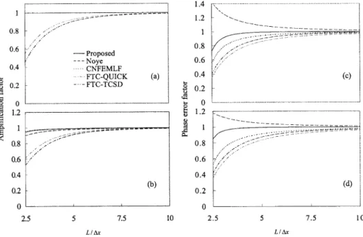
Z1 2⫹Z 2 2 Z ¯ 1 2⫹Z¯ 2 2 (16)The amplification factor depends on three quantities: Courant number, c; diffusion number, s; and wavelength to the grid size ratio, L/⌬x. One can clearly see from Eqs. 共15兲 and 共16兲 that the amplification factor of the proposed scheme is less than or equal to unity when the Courant number is less than or equal to unity. In other words, it is a conditionally stable scheme when the Courant number is less than or equal to unity. Figs. 1共a and b兲 compare the amplification factor of the proposed scheme with that of several schemes for the pure advection case with c⫽0.8, and the disper-sion case with c⫽0.6,s⫽0.06, respectively. Fig. 1共a兲 indicates that the proposed scheme, the Noye scheme共Noye 1990兲, and the CNGFEMLF have no numerical damping for the pure advection process, whereas the fully time-centered implicit QUICK 共FTC-QUICK兲 scheme and the fully time-centered implicit TCSD 共FTC-TCSD兲 scheme produce large numerical diffusion. In addi-tion, Fig. 1共b兲 shows that the proposed scheme and the CNGFEMLF scheme have less numerical damping than all other schemes considered to solve the dispersion equation.
Analysis of Phase Error Factor
Substituting the complex angular frequency
⫽Re共兲⫹ j Im共兲 (17)
into Eq. 共6兲 and considering the real parts of both sides, the propagation velocity of the proposed scheme is
Re共兲 k ⫽ 1 k⌬xtan ⫺1
冉
¯Z2Z1⫺Z¯1Z2 Z ¯1Z1⫹Z¯2Z2冊
(18) The phase error factor, defined as the ratio of the propagation velocity of the proposed scheme to the real velocity U of the analytical solution, becomesRe共兲 kU ⫽ 1 2c L ⌬xtan⫺1
冉
Z ¯2Z1⫺Z¯1Z2 Z ¯1Z1⫹Z¯2Z2冊
(19) Like the amplification factor, the phase error factor is also dependent on Courant number, diffusion number, and the wave-length to grid size ratio. The phase error factors of some schemes considered for the pure advection equation with c⫽0.8 and the dispersion equation with c⫽0.6,s⫽0.06 are displayed in Figs. 1共c and d兲, respectively. One can observe from Figs. 1共c and d兲 that the phase performance of the proposed scheme is the best among the schemes considered. In addition, the Noye scheme generates leading phase errors, whereas the others have lagging ones.Numerical Results
To investigate the computational performances of the proposed scheme, the dispersion equation in various dimensions is solved and compared with other existing numerical schemes.
One-Dimensional Examples Pure Advection in Uniform Flow
A Gaussian concentration distribution is advected for 10,000 s with a uniform velocity U⫽0.8 m/s. A grid space of 100 m and time interval of 100 s are used in this example. The domain of simulation is long enough so that the boundary effect can be ignored. The computed results of various numerical schemes and the exact solution are depicted in Fig. 2 and Table 1 in terms of the maximum and minimum values and the rms errors. From Fig. 2 and Table 1, one can observe that the simulated results by the proposed scheme and the Holly–Preissmann scheme are almost
identical to the exact solution. On the other hand, the other schemes produce large numerical oscillation. Furthermore, the Noye scheme yields leading phase error as shown in the previous stability analysis. The FTC-TCSD scheme and the FTC-QUICK scheme appear to induce large numerical damping.
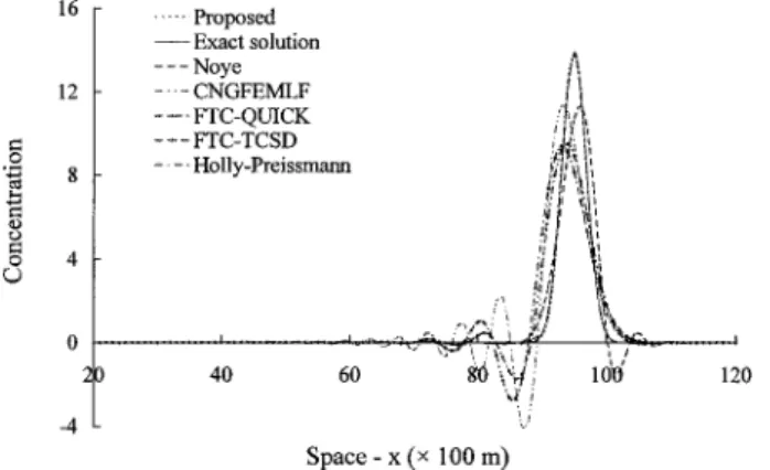
Dispersion in Uniform Flow
The dispersion of a Gaussian concentration distribution with a velocity U⫽0.8 m/s and a diffusion coefficient D⫽0.8 m2/s is simulated for 10,000 s with a grid space of 100 m and time interval of 100 s. Fig. 3 and Table 2 show the proposed scheme produces comparable results compared with a split-operator ap-proach in which the Holly–Preissmann scheme is applied to solve the advection process while the CNSOCDC scheme is applied to the diffusion process. The split-operator CNSOCDC approach used has no numerical oscillation, but its numerical diffusion is larger than that of the proposed scheme. In addition, in compari-son with the other schemes, the proposed scheme has the best computational results.
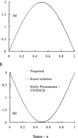
Advection or Dispersion with Variable Velocity
For flow fields with variable velocity, two examples are shown. The first is from Morton and Parrott 共1980兲 with the following pure advection equation:
Fig. 1. 共a兲 Amplification factor portraits c⫽0.8; 共b兲 amplification factor portraits c⫽0.6, s⫽0.006; 共c兲 phase error factor portraits c⫽0.8; and
共d兲 phase error portraits c⫽0.6, s⫽0.06
Fig. 2. Comparison of various schemes for 1D pure advection of Gaussian concentration distribution
Table 1. Performances of Various Schemes in 1D Pure Advection Test
Scheme Max. Min. rms error
Exact solution 11.81 0.0 0.0 Proposed 11.77 ⫺0.002 0.0046 Holly–Preissmann 11.59 ⫺0.003 0.0056 Noye 11.03 ⫺1.540 0.0961 CNGFEMLF 10.24 ⫺2.666 0.1692 FTC-QUICK 8.78 ⫺2.098 0.1948 FTC-TCSD 8.88 ⫺1.324 0.1374
⌽ t ⫹ x
冉
⌽ 1⫹2x冊
⫽0 x苸关0,兴 (20)With the following initial and boundary conditions: ⌽共0,t兲⫽0; ⌽共x,0兲⫽共1⫹2x兲sin 9x, x苸关0,/3兴;
⌽共x,0兲⫽0, x苸关/3,兴 (21) the exact solution for Eq.共20兲 can be derived as
⌽共x,t兲⫽共1⫹2x兲sin 9兵关x2⫹x⫺t⫹1 4兴1/2⫺ 1 2其, for 0⭐x2⫹x⫺t⭐关/3共1⫹/3兲兴 ⌽共x,t兲⫽0, for elsewhere (22) With ⌬x⫽/180 and ⌬t⫽0.3⌬x, simulation results of 80 time steps from the proposed scheme and the CNSOCD scheme, along with the exact solution, are displayed in Fig. 4. Fig. 4 reveals that, despite of little numerical oscillation, the computed results by the proposed scheme are better than those of the CNSOCD scheme.
A second example considers the viscous Burgers equation
⌽t⫹⌽⌽x⫽D⌽xx (23)
Under the initial and boundary conditions of ⌽共x,0兲⫽1 x⭐0
⌽共x,0兲⫽0, x⬎0 (24)
⌽共⫺⬁,t兲⫽1, ⌽共⬁,t兲⫽0, t⬎0 the exact solution to Eq.共23兲 is
⌽共x,t兲⫽
再
1⫹exp冋
1 2␣冉
x⫺ 1 2t冊册
erfc共⫺x/2冑
Dt兲 erfc关共x⫺t兲/2冑
Dt兴冎
⫺1 (25)in which erfc represents the complementary error function. After linearization, the Burgers equation can be solved by the proposed scheme and the numerical simulation results at time t⫽2 s are shown in Fig. 5 under ⌬x⫽0.01 m, ⌬t⫽0.01 s, and D ⫽0.01 m2/s. Fig. 5 shows that the proposed scheme has
satisfac-tory simulation results despite small deviations from the exact solution. It is clearly seen, from the above two numerical ex-amples, that the proposed scheme performs well in flow fields with variable velocity.
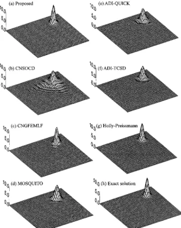
Two-Dimensional Examples Pure Advection in Uniform Flow
A Gaussian concentration distribution with a peak value of 10 and a standard deviation of 220 m is advected for 10,000 s under a constant velocity U⫽0.5 m/s and V⫽0.5 m/s in a two-dimensional infinite domain. The initial central position of this Gaussian distribution is at (x, y )⫽(1,400 m,1,400 m). A grid size of 100 m⫻100 m and time step of 100 s are used to conduct the simulation. Figs. 6共a–h兲 show the bird’s-eye view of the com-puted results from several numerical schemes. Table 3 displays the maximum and minimum values and the rms errors for each scheme used. In addition, the computed concentration profiles by different schemes along the line y⫽x are shown in Fig. 7. It is observed that the computed results by the proposed scheme关Fig. 6共a兲兴 and the Holly–Preissmann scheme 关Fig. 6共g兲兴 almost agree with the exact solution. The Holly–Preissmann scheme has the Fig. 3. Comparison of various schemes for 1D dispersion of
Gauss-ian concentration distribution
Fig. 4. Computational results of pure advection equation with varia-tion of velocity
Fig. 5. Computational results of 1D viscous Burgers equation using the proposed scheme
Table 2. Performances of Various Schemes in 1D Dispersion Test
Scheme Max. Min. rms error
Exact solution 13.91 0.0 0.0 Proposed 13.81 ⫺0.057 0.0123 Holly–Preissmann⫹CNSOCD 13.75 0.0 0.0065 Noye 11.32 ⫺1.401 0.1127 CNGFEMLF 11.31 ⫺3.996 0.2648 FTC-QUICK 9.38 ⫺2.680 0.2490 FTC-TCSD 9.48 ⫺1.755 0.1837
least numerical oscillation among all the schemes considered, however, its numerical damping is larger than that of the proposed scheme. The CNSOCD scheme关Fig. 6共c兲兴 produces very severe numerical oscillation that rapidly spreads over the modeling do-main. The ADI-QUICK scheme 共Chen and Falconer 1992兲 关Fig. 6共e兲兴, the ADI-TCSD scheme 共Chen and Falconer 1994兲 关Fig. 6共f兲兴, and the MOSQUITO scheme 关Fig. 6共d兲兴 共Balzano 1999兲 seem to produce results with large numerical damping. The CNGFEMLF scheme 关Fig. 6共b兲兴 has smaller numerical diffusion than those of the ADI-QUICK scheme, the ADI-TCSD scheme, and the MOSQUITO scheme. However, its numerical oscillation is large in comparison with the other three schemes.
Dispersion in Uniform Flow
Consider a 2D nondimensional dispersion equation with uniform flow velocity as
⌽t⫹⌽x⫹⌽x⫽D共⌽xx⫹⌽y y兲 (26)
where D⫽inverse of the Reynolds number. Under the initial con-dition
⌽共x, y ,0兲⫽sin共x兲⫹sin共y兲. (27) and the boundary conditions
⌽共0,y ,t兲⫽关sin共⫺t兲⫹sin 共y⫺t兲兴exp共⫺D2t兲 ⌽共1,y ,t兲⫽关sin共1⫺t兲⫹sin 共y⫺t兲兴exp共⫺D2t兲
(28) ⌽共x,0,t兲⫽关sin共x⫺t兲⫹sin共⫺t兲兴exp共⫺D2t兲
⌽共x,1,t兲⫽关sin共x⫺t兲⫹sin 共1⫺t兲兴exp共⫺D2t兲 the exact solution to Eq.共26兲 is
⌽共x, y ,t兲⫽关sin共x⫺t兲⫹sin 共y⫺t兲兴exp共⫺D2t兲 (29) Numerical results by the proposed scheme and a split-operator approach are shown in Figs. 8共a and b兲 at t⫽2 and t⫽3 along the line y⫽x with D⫽0.0002, a uniform grid size of 0.02⫻0.02, and time step of 0.01. In the split-operator approach, the Holly– Preissmann scheme and the Crank–Nicholson second-order cen-tral difference scheme are used to solve the advection and the diffusion processes, respectively. Figs. 8共a and b兲 demonstrate that the simulated results by the proposed scheme and the split-operator approach are almost identical to the exact solution. It must be noticed that the use of the proposed scheme to the 2D dispersion equation is straightforward by adopting the method of fractional steps. However, the application of a split-operator ap-proach is more expensive and complicated since the advection and diffusion processes are computed separately. Furthermore, the additional equations of spatial derivative must be computed in the Holly–Preissmann scheme for solving the dispersion equation. Pure Advection in Rigid-Body Rotating Flow
A pure advection of a Gaussian concentration distribution with a rigid-body rotating flow in a two-dimensional infinite domain is considered. This problem has a flow field of variable velocity. The maximum value and the standard deviation of this Gaussian con-centration distribution are unity and 250 m, respectively. The rigid body spends 20,000 s rotating one turn. A grid size of 100 m⫻100 m and time step of 50 s are used in numerical simu-lation. After one rotation, the maximum and minimum values of the computational results by the proposed scheme are 0.986 and ⫺0.012, respectively. This numerical example shows that the pro-posed scheme also has good capability to accurately solve the two-dimensional problem with variable velocity.
Fig. 6. Comparison of various schemes for 2D pure advection with uniform flow
Fig. 7. Comparison of various schemes for 2D pure advection with uniform flow共along line y⫽x兲
Table 3. Performances of Various Schemes in 2D Pure Advection Test
Scheme Max. Min. rms error
Exact solution 10.00 0.0 0.0 Proposed 9.87 ⫺0.010 0.0017 Holly–Preissmann 9.60 ⫺0.008 0.0017 CNSOCD 5.94 ⫺2.517 0.1000 CNGFEMLF 9.05 ⫺1.719 0.0195 MOSQUITO 6.62 ⫺0.959 0.0261 ADI-QUICK 6.96 ⫺0.957 0.0278 ADI-TCSD 6.81 ⫺0.431 0.0173
Three-Dimensional Example
Three-Dimensional Diffusion in A Shear Flow
To investigate the capability of the proposed scheme for solving three-dimensional problems, diffusion in a shear flow is consid-ered. The velocity shear in the diffusion of a patch of passive contaminant from an instantaneous source plays an important role in groundwater flow or natural streams such as ocean, lake, and estuaries. The governing equation for shear diffusion can be ex-pressed as
⌽t⫹共V0⫹⍀yy⫹⍀zz兲⌽x⫽Dx⌽xx⫹Dy⌽y y⫹Dz⌽zz (30) where V0⫽mean velocity in the x direction; ⍀y and ⍀z
⫽horizontal and vertical shear, respectively; and Dx, Dy, and
Dz⫽eddy diffusivities in x, y, and z directions, respectively. The
analytical solution for an instantaneous point source of mass M released at x⫽y⫽z⫽0 was obtained by Carter and Okubo 共1965兲 as ⌽共x,y ,z,t兲⫽ M 83/2共D xDyDz兲1/2t3/2共1⫹2t2兲1/2 exp ⫺
冋
共x⫺V0t⫺0.5共⍀yy⫹⍀zz兲t兲 2 4Dxt共1⫹2t2兲 ⫹ y 2 4Dyt ⫹ z 2 4Dzt册
(31) where 2⫽b共⍀y 2 Dy/Dx兲⫹共⍀z 2 Dz/Dx兲c 12 (32)Allowing numerical solution having an initial peak concentra-tion of unity, simulaconcentra-tion begins at time t⫽t0 having the point
source of mass M as
M⫽83/2共DxDyDz兲1/2t3/2共1⫹2t02兲1/2 (33) In the numerical simulation the following parameters are used: t0⫽1000 s, V0⫽0.5 m/s, ⍀y⫽⍀z⫽0.0003 1/s, Dx⫽Dy⫽Dz
⫽5.0 m2/s, ⌬t⫽100 s, and grid space ⌬x⫽⌬y⫽⌬z⫽100 m.
Fig. 9 shows the contour plots of the proposed scheme and the analytical solution at t⫽3,000 and 5,000 s on the plane z⫽0, respectively. The proposed scheme yields the results that are al-most in excellent agreement with the exact solution.
Conclusions
In this article, a hybrid finite-difference scheme capable of solv-ing pure advection, pure diffusion, and dispersion processes is proposed. The proposed scheme combines two well-known schemes, namely, the Crank–Nicholson second-order central dif-ference scheme and the Crank–Nicholson Galerkin finite-element method with linear basis functions. The consistency and stability of the proposed scheme are investigated. In addition, the relations between the modified equations corresponding to the proposed scheme and the two selected schemes are obtained. Employing the method of fractional steps, the proposed scheme that was originally developed for one-dimensional problems can be ap-plied straightforwardly to multidimensional ones without much difficulty. The proposed scheme has the best performance in sev-eral examples among some non-split-operator schemes. In addi-tion, the proposed scheme yields comparable results in compari-son with a well-known and accurate split-operator approach in which the Holly–Preissmann scheme and the Crank–Nicholson second-order central difference scheme were used to solve advec-tion and diffusion processes, respectively. The proposed scheme is a non-split-operator approach and, therefore, it has the advan-tage of being simpler and more efficient than the split-operator approach.
Acknowledgments
The writers would like to express their appreciation for the sup-port from the National Science Council of the R.O.C. under Grant No. NSC88-2211E0002-51 and the SINOTECH Foundation for Research and Development of Engineering Sciences and Tech-nologies.
Fig. 8. Computational results of 2D dispersion equation共along line
y⫽x兲: 共a兲 t⫽2 and 共b兲 t⫽3
Fig. 9. Comparison of contour plots of diffusion in shear flow on plane z⫽0 at t⫽3000 and 5000 s
Appendix: Consistency and Modified Equation Consistency
Applying any two-level numerical schemes to Eq. 共1兲, one may obtain the following discretization equations:
a1⌽in⫹1⫺2⫹a2⌽in⫹1⫺1⫹a3⌽in⫹1⫹a4⌽in⫹1⫹1⫹a5⌽in⫹1⫹2 ⫽b1⌽i⫺2n ⫹b2⌽i⫺1n ⫹b3⌽i
n⫹b
4⌽i⫹1n ⫹b5⌽i⫹2n (34) and
c1⌽i⫺2n⫹1⫹c2⌽i⫺1n⫹1⫹c3⌽in⫹1⫹c4⌽i⫹1n⫹1⫹c5⌽i⫹2n⫹1 ⫽d1⌽i⫺2n ⫹d2⌽i⫺1n ⫹d3⌽i
n⫹d
4⌽i⫹1n ⫹d5⌽i⫹2n (35) where a1⫹a2⫹a3⫹a4⫹a5⫽c1⫹c2⫹c3⫹c4⫹c5⫽1. The ⌽in⫹1
represents the value of ⌽ at grid point i for time level t⫽(n ⫹1)⌬t and ⌬t is the time step. The terms ⌽in⫹1⫹1,⌽ni⫹1, ⌽in⫺1⫹1,
⌽in⫹1, and⌽in⫺1can be expanded in Taylor series as
⌽i⫹ j 1 n⫹k1⫽
兺
m⫽0 ⬁ 1 m!冉
k1⌬t t ⫹j1⌬x x冊
m ⌽i n k 1, j1⫽⫺1,0,1 (36) where⌬x⫽grid size. Substitution of Eq. 共36兲 into Eqs. 共34兲 and 共35兲 yields⌽t⫽A1⌽x⫹A2⌽tt⫹A3⌽tx⫹A4⌽xx⫹A5⌽ttt⫹A6⌽ttx⫹A7⌽txx
⫹A8⌽xxx⫹¯ (37)
and
⌽t⫽B1⌽x⫹B2⌽tt⫹B3⌽tx⫹B4⌽xx⫹B5⌽ttt⫹B6⌽txx⫹B7⌽txx
⫹B8⌽xxx⫹••• (38)
where the superscript n and the subscript i for⌽ are eliminated. The terms A1⬃A8 and B1⬃B8 are functions of a1⫺a5, b1⫺b5
and c1⫺c5, d1⫺d5, respectively. For example, A2and A3can be
expressed as A2⫽
⫺⌬t
2 共a1⫹a3⫹a4⫹a5兲⫽ ⫺⌬t
2 (39)
A3⫽⌬x共2a1⫹a2⫺a4⫺2a5兲 (40) As far as the accuracy is concerned, both A1and B1are equal to
⫺U. In addition, because of the consistency, the terms A2⬃A8
and B2⬃B8, except A4 and B4, are all equal to zeros when⌬t
and⌬x approach zero. However, A4and B4satisfy the following
condition:
A4⫽B4⫽D (41)
where D⫽diffusion coefficient. Now, taking the linear combina-tion of Eqs. 共34兲 and 共35兲 as ␣ 关Eq. 共34兲兴⫹ 关Eq. 共35兲兴, one obtains
共␣a1⫹c1兲⌽in⫺2⫹1⫹共␣a2⫹c2兲⌽in⫺1⫹1⫹共␣a3⫹c3兲⌽i n⫹1
⫹共␣a4⫹c4兲⌽i⫹1n⫹1⫹共␣a5⫹c5兲⌽i⫹2n⫹1
⫽共␣b1⫹d1兲⌽i⫺2n ⫹共␣b2⫹d2兲⌽i⫺1n ⫹共␣b3⫹d3兲⌽i n
⫹共␣b4⫹d4兲⌽i⫹1n ⫹共␣b5⫹d5兲⌽i⫹2n (42) where ␣ and  are constants. Similarly, substitution of Taylor series expansion共36兲 into Eq. 共42兲 yields
⌽t⫽⫺U⌽x⫹ 1
␣⫹关共␣A2⫹B2兲⌽tt⫹共␣A3⫹B3兲⌽tx ⫹共␣A4⫹B4兲⌽xx⫹共␣A5⫹B5兲⌽ttt共␣A6⫹B6兲⌽ttx ⫹共␣A7⫹B7兲⌽txx⫹共␣A8⫹B8兲⌽xxx兴⫹¯ (43) One can clearly see from Eq.共43兲 that Eq. 共42兲 is also consistent with the dispersion equation共1兲.
Modified Equation
By eliminating pure and cross time derivatives with repeatedly differentiating Eqs. 共37兲 and 共38兲, the modified equation corre-sponding to Eqs.共37兲 and 共38兲 can, respectively, be expressed as ⌽t⫽⫺U⌽x⫹E2⌽xx⫹E3⌽xxx⫹¯ (44) and
⌽t⫽⫺U⌽x⫹F2⌽xx⫹F3⌽xxx⫹¯ (45) where
E2⫽U2A2⫺UA3⫹A4
E3⫽⫺2U3A2 2⫹3U2A 2A3⫺2UA2A4⫺UA3 2⫹A 3A4⫺U3A5 ⫹U2A 6⫺UA7⫹A8 (46) and F2⫽U2B2⫺UB3⫹B4 F3⫽⫺2U3B2 2⫹3U2B 2B3⫺2UB2B4⫺UB3 2
⫹B3B4⫺U3B5⫹U2B6⫺UB7⫹B8 (47) Similarly, the modified equation corresponding to Eq.共43兲 is
⌽t⫽⫺U⌽x⫹ G2 ␣⫹ ⌽xx⫹ G3 ␣⫹ ⌽xxx⫹¯ (48) where
G2⫽U2共␣A2⫹B2兲⫺U共␣A3⫹B3兲⫹共␣A4⫹B4兲 (49)
G3⫽ 1
␣⫹关⫺2U3共␣A2⫹B2兲2⫹3U2共␣A2⫹B2兲 ⫻共␣A3⫹B3兲⫺2U共␣A2⫹B2兲共␣A4⫹B4兲 ⫺U共␣A3⫹B3兲2⫹共␣A3⫹B3兲共␣A4⫹B4兲兴 ⫺U3共␣A
5⫹B5兲⫹U2共␣A6⫹B6兲 ⫺U共␣A7⫹B7兲⫹共␣A8⫹B8兲 It is obvious that G2, E2, and F2 satisfy
G2⫽␣E2⫹F2 (50)
In addition, if A2, B2, A3, and B3 satisfy the following
condi-tions:
A2⫽B2 (51)
and
A3⫽B3 (52)
one can obtain
G3⫽␣E3⫹F3 (53)
In other words, Eq.共48兲 can be rewritten as
共␣⫹兲⌽t⫽⫺U共␣⫹兲⌽x⫹共␣E2⫹F2兲⌽xx
⫹共␣E3⫹F3兲⌽xxx⫹¯ (54) It is necessary to point out that condition共51兲 is always satisfied due to Eq. 共39兲. Eq. 共52兲 is a sufficient condition for Eq. 共53兲. Although the above derivation is only up to the third-order de-rivative, the higher-order derivative can also be executed in the same manner.
Notation
The following symbols are used in this paper: a1⫺a3,b1⫺b3,
c1⫺c3,d1⫺d3 ⫽ coefficients of discretized
equation; A1⫺A8,B1⫺B8,
E1⫺E8,F1⫺F8 ⫽ function of a1⫺a3,b1
⫺b3,c1⫺c3,d1⫺d3;
c ⫽ Courant number; D,Dx,Dy,Dz ⫽ diffusion coefficient or
the inverse of Rey-nolds number; G2G3 ⫽ function of A1⫺A8,B1 ⫺B8; j ⫽ an imaginary unit; k ⫽ wave number; L ⫽ wavelength; M ⫽ mass of concentration; s ⫽ diffusion number; U,V ⫽ velocity component;
W ⫽ amplitude of wave; Z1,Z2,Z¯1,Z¯2 ⫽ function of c, s, k, and ⌬x; ␣,  ⫽ constant; ⌬t ⫽ time increment; ⌬x ⫽ computational grid interval; ⌽ ⫽ temperature or concen-tration; and
⍀y,⍀z ⫽ horizontal and vertical
shears. Subscripts
i ⫽ x-directional computational point index; and m ⫽ index of an mth wave component.
Superscripts
n ⫽ time step index. References
Balzano, A.共1999兲. ‘‘MOSQUITO: An efficient finite-difference scheme for numerical simulation of 2D advection.’’ Int. J. Numer. Methods Fluids, 31, 481– 496.
Bradley, D., and Missaghi, M.共1988兲. ‘‘A Taylor-series approach to nu-merical accuracy and a third-order scheme for strong convective flows.’’ Comput. Methods Appl. Mech. Eng., 69, 133–151.
Cater, H. H., and Okubo, A.共1965兲. ‘‘A study of the physical process of movement and dispersion in the Cape Kennedy area.’’ Final Rep. U.S. Am. Energy Comm. Contract No. AT (30-1).
Chen, Y., and Falconer, R. A. 共1992兲. ‘‘Advection–diffusion modeling using the modified QUICK scheme.’’ Int. J. Numer. Methods Fluids, 15, 1171–1196.
Chen, Y., and Falconer, R. A.共1994兲. ‘‘Modified forms of the third-order convection second-order diffusion scheme for the advection–diffusion equation.’’ Adv. Water Resour., 17, 147–17.
Gaskell, P. H., and Lau, A. K. C.共1988兲. ‘‘Curvature compensated con-vective transport: SMART, a new boundedness preserving transport algorithm.’’ Int. J. Numer. Methods Fluids, 8, 617– 641.
Gersho, P. M., and Sani, R. L.共1998兲. Incompressible flow and the finite-element method, Wiley, Chichester, England, Vol. 1.
Holly, F. M., Jr., and Preissmann, A. 共1977兲. ‘‘Accurate calculation of transport in two dimensions.’’ J. Hydraul. Eng., 103共11兲, 1259–1277. Komatsu, T., Ohgushi, K., and Asai, K. 共1997兲. ‘‘Refined numerical scheme for advective transport in diffusion simulation.’’ J. Hydraul. Eng., 123共1兲, 41–50.
Leonard, B. P.共1979兲. ‘‘A stable and accurate convective modeling pro-cedure based on quadratic upstream interpolation.’’ Comput. Methods Appl. Mech. Eng., 19, 59–98.
Leonard, B. P. 共1988兲. ‘‘Simple high-accuracy resolution program for convective modeling of discontinuities.’’ Int. J. Numer. Methods Flu-ids, 8, 1291–1318.
Leonard, B. P., and Noye, B. J.共1990兲. ‘‘Second- and third-order two-level implicit FDM’s for unsteady one-dimensional convection diffu-sion.’’ Computational techniques and applications: CTAC-89, Hemi-sphere, New York, 311–317.
Li, S. G., Ruan, F., and Mclaughlin, D.共1992兲. ‘‘A space–time accurate method for solving solute transport problems.’’ Water Resour. Res., 28, 2297–2306.
Morton, K. W., and Parrott, A. K.共1980兲. ‘‘Generalize Galerkin methods for first-order hyperbolic equation.’’ J. Comput. Phys., 36, 249–270. Noye, B. J. 共1986兲. ‘‘Finite-difference methods for solving the
one-dimensional transport equation,’’ in Numerical modelling— applications to marine systems, B. J. Noye, ed., North-Holland Math-ematics Studies Vol. 134, North-Holland, Dordrecht, pp. 231–256. Noye, B. J.共1990兲. ‘‘A new third-order finite-difference method for
tran-sient one-dimensional advection diffusion.’’ Commun. Appl. Numer. Methods, 6, 279–288.
Roe, P. L. 共1981兲. ‘‘Approximate Riemann solvers, parameter vectors, and difference schemes.’’ J. Comput. Phys., 43, 357–372.
Van Leer, B. 共1977兲. ‘‘Towards the ultimate conservative difference scheme. IV. A new approach to numerical convection.’’ J. Comput. Phys., 23, 276 –299.
Wang, J. C. T., and Windhopf, G. F. 共1989兲. ‘‘A high-resolution TVD finite-volume scheme for Euler equations in conservation form.’’ J. Comput. Phys., 84, 145–173.
Warming, R. F., and Hyett, B. J. 共1974兲. ‘‘The modified equation ap-proach to the stability and accuarcy analysis of finite-difference meth-ods.’’ J. Comput. Phys., 14, 159–179.
Yaneko, N. N. 共1971兲. The method of fractional steps: the solution of problems of mathematical physics in several variables, Springer, New York.