Mining Frequent Itemsets from Data Streams with a Time-Sensitive Sliding Window
Chih-Hsiang Lin Ding-Ying Chiu Yi-Hung Wu [email protected] [email protected] [email protected]
Department of Computer Science National Tsing Hua University
Hsinchu, Taiwan 300, R.O.C.
Arbee L. P. Chen* [email protected] Department of Computer Science
National Chengchi University Taipei, Taiwan, R.O.C.
Abstract
Mining frequent itemsets has been widely studied over the last decade. Past research focuses on mining frequent itemsets from static databases. In many of the new applications, data flow through the Internet or sensor networks. It is challenging to extend the mining techniques to such a dynamic environment. The main challenges include a quick response to the continuous request, a compact summary of the data stream, and a mechanism that adapts to the limited resources. In this paper, we develop a novel approach for mining frequent itemsets from data streams based on a time-sensitive sliding window model. Our approach consists of a storage structure that captures all possible frequent itemsets and a table providing approximate counts of the expired data items, whose size can be adjusted by the available storage space. Experiment results show that in our approach both the execution time and the storage space remain small under various parameter settings. In addition, our approach guarantees no false alarm or no false dismissal to the results yielded.
1 Introduction
Data items continuously flow through the Internet or sensor networks in applications like network monitoring and message dissemination. Efforts have been made at providing a data stream management system (DSMS), e.g., Telegraph [6], STREAM [25], Niagara [11], and Aurora [1]. The characteristics of data streams are as follows [4][17]:
1. Continuity: Data continuously arrive at a high rate.
2. Expiration: Data can be read only once.
3. Infinity: The total amount of data is unbounded.
The above leads to the following requirements: 1. Time-sensitivity: A model that adapts itself to the
time passing of a continuous data stream is needed. 2. Approximation: Because the past data cannot be
stored, a method for providing the approximate answers with accuracy guarantees is required. 3. Adjustability: Owing to the unlimited amount of
data, a mechanism that adapts itself to available resources is needed.
*To whom all the correspondence should be sent.
Among the researches toward DSMS, extending mining techniques to data streams has attracted much attention [19][26][28][10][27]. In this paper, we focus on the problem of mining frequent itemsets over a data stream. In this problem, a data stream is formed by transactions arriving in series. The support count of an itemset means the number of transactions containing it and a frequent itemset means the one with a sufficient support count.
Mining frequent itemsets in static databases has been widely studied over the last decade. Many methods such as Apriori [2], FP-growth [18], and OpportuneProject [23] have been proposed. In addition, the methods that incrementally mine frequent itemsets in dynamic databases [12][22][8] have been presented as well. In these methods, all the frequent itemsets and their support counts derived from the original database are retained. When transactions are added or expired, the support counts of the frequent itemsets contained in them are recomputed. By reusing the frequent itemsets and their support counts retained, the number of candidate itemsets generated during the mining process can be reduced. All these methods have to rescan the original database because non-frequent itemsets can be frequent after the database is updated. Therefore, they cannot work without seeing the entire database and cannot be applied to data streams.
Recent works on mining frequent itemsets over data streams are classified into two groups, mining frequent items and mining frequent itemsets. Most of them [15][21][24] utilize all the data between a particular point of time (called landmark) and the current time for mining. The landmark usually refers to the time when the system starts. Moreover, the support count of an itemset in this model is the number of transactions containing it between the landmark and the current time. The landmark model is illustrated in Figure 1.
Figure 1: Landmark model
To find frequent items [15][21][24] under this model, the support count of each incoming item is
accumulated on a counter. Since the number of distinct items is often more than available counters, sampling techniques are employed to assign items to counters and then estimate the support counts of all the items.
For mining frequent itemsets, Lossy-counting [24] is the representative approach under the landmark model. It keeps monitoring the maximum possible count of each itemset in the past data, called the maximum possible error. Given an error tolerance parameter and a support count threshold, this approach computes the approximate count of each itemset with an accuracy guarantee and regards the itemsets whose approximate counts exceed the support count threshold as frequent. Since the approximate count of an itemset keeps growing as time goes by, the support count threshold is also increasing along the time axis.
All these approaches satisfy one requirement mentioned above – approximation. However, in many applications, new data are often more important than old ones. For example, when mining the Web click streams, the most recent data usually provides more useful information than those that arrived previously. The landmark model is not aware of time and therefore cannot distinguish between new data and old ones. To overcome this difficulty, the time-fading model, a variation of the landmark model, has been presented in recent works [7][13][16]. It assigns different weights to transactions such that new ones have higher weights than old ones. As shown in Figure 2, the weights are decreasing as time passes by.
Figure 2: Time-fading model
The estDec method in [7] is proposed for mining frequent itemsets under this model. By using a decay rate, the effects of old transactions diminish as time goes by. For example, let the decay rate and the support count of itemset X be d and v, respectively. As a new transaction containing X arrives, the new support count of X is equal to v×d+1. Obviously, when d equals 1, the time-fading model becomes the landmark model. In [13], a variety of decay functions are also introduced to maintain aggregates under the time-fading models.
FP-stream approach in [16] provides a way to mine frequent itemsets under the time-fading model. Two parameters, the minimum support count σ and the maximum support error ε where σ ≥ ε, are used to classify all the itemsets into three categories:
• Frequent: Support count is greater than and equal
to σ.
• Sub-frequent: Support count falls in [ε, σ].
• Infrequent: Support count is smaller than ε.
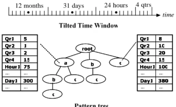
Next, only frequent and sub-frequent itemsets are stored and organized as a pattern tree, a variation of the FP-tree [18]. Figure 3 shows a pattern tree, where a path starting at the root stands for an itemset. The count of each itemset is asymmetrically distributed into multiple time slots such that the recent time period is assigned more time slots than the past. The assignment of time slots is illustrated by the tilted time window shown in Figure 3. It is suitable for people to mine the recent data at a fine granularity while mining the long-term data at a coarse granularity.
4 qtrs 24 hours 31 days
12 months
time
Figure 3: Pattern tree and Tilted-time window All these approaches provide approximate answers for long-term data and adjust their storage requirement based on the available space. Therefore, they satisfy the two requirements – approximation and adjustability. However, the time-fading model (including the landmark model) has its essential limitation, i.e., the support count is computed from the entire data set between the landmark and the current time. In certain applications, users can only be interested in the data recently arriving within a fixed time period. Obviously, the models previously presented are unable to satisfy this need. On the contrary, the sliding-window model shown in Figure 4 achieves this goal. Given a window size W, only the latest W transactions are utilized for mining. As a transaction arrives, the oldest transaction in the sliding window is expired. Therefore, under this model, the methods for finding the expired transaction and for discounting the support counts of the itemsets involved are required.
Figure 4: Sliding-window model
Babcock et al. [5] develop a mechanism, which can dynamically combine adjacent buckets in a histogram, to monitor the variance and k-medians in a sliding
window. In [9][14][20], hash-based methods are proposed to mine frequent items. In these methods, a fixed number of counters and hashing functions are used. An item is then assigned to the corresponding counters based on its hashed values. Each counter accumulates the support counts of the items with the same value hashed. In this way, the support count of an item can be estimated from the corresponding counters. Since these methods assume the expired transaction to be available, the update of these counters can be fast. However, the characteristic – expiration, said that it is not reasonable to have a chance to see the expired transaction again. In a recent work, Arasu and Manku [3] extend the Lossy-counting to the sliding-window model. Their approach can estimate the approximate counts and quantiles with certain accuracy guarantees.
Compared with the previous models considering only the insertion of transactions, the sliding-window model further considers the deletion of transactions. Therefore, if a method succeeds in the sliding-window model, it can be easily applied to the previous models. Moreover, all the previous works consider a fixed number of transactions as the basic unit for mining, which is not easy for people to specify. By contrast, it is natural for people to specify a time period as the basic unit. Therefore, in this paper, we propose the time-sensitive sliding-window model, which regards a fixed time period as the basic unit for mining.
Definition 1.1 Time-sensitive Sliding-window (TS)
Given a time point t and a time period p, the set of all the transactions arriving in [t-p+1, t] will form a basic block. A data stream is decomposed into a sequence of basic blocks, which are assigned with serial numbers starting at 1. Given a window with length |W|, we slide it over this sequence to see a set of overlapping sequences, where each sequence is called the time-sensitive sliding-window abbreviated as TS.
Let the basic block numbered i be denoted as Bi.
The number of transactions in Bi is denoted as |Bi|,
which is not fixed due to the variable data arrival rate. For each Bi, the TS that consists of the |W| consecutive basic blocks from Bi-|W|+1 to Bi is denoted as TSi. Let
the number of transactions in TSi be denoted as ∑i. Definition 1.2 Frequent Itemsets in TSi/Bi
The support count of an itemset in TSi (Bi) is the number of transactions in [Bi-|W|+1, … Bi] (Bi) containing it. Given the support threshold θ, an itemset is frequent in TSi (Bi) if its support count in TSi (Bi) is not smaller than θ×∑i (θ×|Bi|).
Owing to the characteristics of data streams, it is not realistic to scan the past basic blocks again and again for mining frequent itemsets in each of the subsequent TS’s. In this paper, we assume that only the summary information derived from TSi-1 is provided for mining frequent itemsets in TSi. Such a scenario is illustrated
in Figure 5, where the basic unit is one day and |W| is 3. As the new basic block B6/21 comes, the oldest basic block B6/18 in TS6/20 is expired. To find frequent itemsets in TS6/21, we consider three kinds of itemsets from two sources, the frequent itemsets in TS6/20 and the frequent ones in B6/21, as follows:
• For each frequent itemset in TS6/20, the support count is discounted if it occurs in B6/18 and then updated by examining B6/21. A mechanism to keep its support count in B6/18 and a way to find its support count in B6/21 are needed.
• A frequent itemset in B6/21, which is not frequent in TS6/20, can be frequent in TS6/21. The methods for computing its support count in TS6/20 and for mining frequent itemsets in B6/21 are required.
• An itemset that is not frequent in both TS6/20 and B6/21 cannot be frequent in TS6/21.
Figure 5: Time-sensitive sliding-window model Since all the methods developed under other models accumulate the support count for each frequent itemset, no discounting information is provided. Furthermore, the hash-based approaches for mining frequent items under the sliding-window model assume that the expired transactions are available. However, for mining frequent itemsets, it is not reasonable to allow that the expired transactions can be reexamined. Therefore, in this paper, we introduce a novel approach to address the issues described above. First of all, we devise a data structure named the discounting table (DT) to retain the frequent itemsets with their support counts in the individual basic blocks of the current TS. Moreover, a data structure named the Potentially Frequent-itemset Pool (PFP) is used to keep the frequent itemsets in TSi and the frequent ones in Bi. We include the itemsets that are frequent in Bi but not frequent in TSi-1 in PFP because they are possibly frequent in TSi.
Definition 1.3 Potentially Frequent Itemset
A frequent itemset in Bi that is not frequent in TSi-1 is called a potentially frequent itemset. Since its support count in TSi-1 is not recorded, we estimate that as the
largest integer less than θ×∑i-1, i.e., the upper bound of its support count in [Bi-|W|, … Bi-1]. This is called the potential count and also recorded in PFP.
For the itemsets in PFP that are not potentially frequent, the potential counts are set to 0. In this way, each itemset in PFP is associated with the potential count and the accumulated count. Moreover, the sum of the two counts is regarded as the support count of this itemset in TSi and used to determine whether it should be kept in PFP. When Bi arrives, three pieces of information are available for mining and discounting:
• DT: Frequent itemsets with support counts in each of the basic blocks Bi-|W|, … Bi-1.
• PFP: Frequent itemsets in TSi-1 or Bi-1.
• All the frequent itemsets discovered from Bi. Mining frequent itemsets in TSi consists of four steps. At first, the support counts of frequent itemsets in PFP are discounted according to DT and then the frequent itemsets in Bi-|W| are removed from DT. Second, the frequent itemsets in Bi are mined by using FP-growth [18] and added into PFP with their potential counts computed. Third, for each itemset that is in PFP but not frequent in Bi, we scan Bi to accumulate its support count and then delete it from PFP if it is not frequent in TSi. At last, two alternatives to determine the frequent itemsets for output are provided:
1. Recall-oriented: All the itemsets kept in PFP are
output. Since all the frequent itemsets in TSi are in PFP, it guarantees that no false dismissal occurs. 2. Precision-oriented: We output only those itemsets
whose accumulated counts in PFP satisfy θ×∑i. Because for the potentially frequent itemsets, these counts are lower bounds of their support counts, it guarantees that no false alarm occurs.
In addition to the mining and discounting methods, we further design the self-adjusting discounting table (SDT) that can automatically adjust its size when maintaining the discounting information. Given a limitation on the size of SDT, we devise a strategy to merge the information of more than one itemset kept in SDT. The main idea is to minimize the difference between the original support count of each itemset and its approximate count after merging. The most important finding is that the two guarantees described above still hold when SDT is deployed. The following are the contributions of our paper, corresponding to the three requirements mentioned before.
• Time-sensitive sliding-window model: We propose
a model that is sensitive to time. To our knowledge, this paper is the first one addressing the issues of mining frequent itemsets over data streams under this model.
• Mining and discounting methods: An approach
that continuously provides frequent itemsets over data streams under our model is introduced. The
accuracy guarantees of no false dismissal or no false alarm are provided.
• Self-adjusting discounting table: A mechanism
that is self-adjusting under the memory limitation is presented. The accuracy guarantees still hold. The remainder of this paper is organized as follows. Section 2 details the mining and discounting methods, including the system framework and main operations. In Section 3, we present the self-adjusting discounting table. The experiment results are shown and discussed in Section 4. In Section 5, we conclude this paper.
2 Mining
and
Discounting
2.1 System
framework
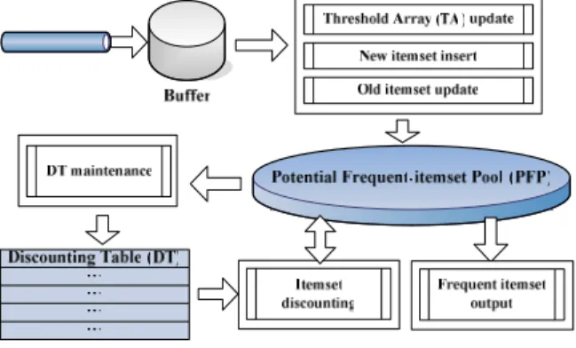
Figure 6 shows the system framework of our approach. The data stream is a series of transactions arriving continuously. Four parameters, the support threshold θ, the basic unit of time period for each basic block P, the length of TS |W|, and the output mode M, are given before the system starts. As Definition 1.1 states, a data stream is divided into blocks with different numbers of transactions according to P. The buffer continuously consumes transactions and pours them block-by-block into our system. After a basic block triggers these operations and goes through our system, it will be discarded directly.
Figure 6: System framework
Because the basic blocks may have different numbers of transactions, we dynamically compute the support count threshold θ×|Bi| for each basic bock Bi and store it into an entry in the threshold array (TA), denoted as TA[i]. In our approach, only |W|+1 entries are maintained in TA. As Bi arrives, TA[j] keeps the support count threshold of Bi-j for 1≤j≤|W|+1 and i-j>0. After Bi is processed, the last entry TA[|W|+1] is ignored and the others are moved to the next positions, i.e., TA[j]→TA[j+1] for 1≤j≤|W|. Finally, the support count threshold of Bi is put into TA[1].
In addition to TA_update, the arrival of a basic block also triggers the other operations in Figure 6, which are differently executed in three cases. For each case, Frequent_itemset_output is used to pick up the
answers satisfying M from PFP. Figure 7 shows the main algorithm. First, as B1 comes, two operations are executed one by one:
• New_itemset_insertion: An algorithm for mining
frequent itemsets is applied to the transactions in the buffer. Each frequent itemset is inserted into PFP in the form of (ID, Items, Acount, Pcount), recording a unique identifier, the items in it, the accumulated count, and the potential count, respectively. Since an itemset is added into PFP, Acount accumulates its exact support counts in the subsequent basic blocks, while Pcount estimates the maximum possible sum of its support counts in the past basic blocks. For B1, Pcount is set as 0.
• DT_maintenance: Each itemset in PFP is inserted
into DT in the form of (B_ID, ID, Bcount), recording the serial number of the current basic block, the identifier in PFP, and its support count in the current basic block, respectively. For B1, B_ID is set as 1.
Input: Stream S, Parameters θ, P, |W|, M Output: All the frequent itemsets satisfying M
1. Let TA, PFP, and DT be empty //∀j, TA[j]=0 2. While Bi comes //from the buffer 2.1 If (i = 1) //B1 2.1.1 New_itemset_insertion 2.1.2 DT_maintenance 2.2 Else If (i ≤ |W|) //B2…B|W| 2.2.1 New_itemset_insertion 2.2.2 Old_itemset_update 2.2.3 DT_maintenance 2.3 Else //B|W|+1… 2.3.1 Itemset_discounting 2.3.2 New_itemset_insertion 2.3.3 Old_itemset_update 2.3.4 DT_maintenance
2.4 TA_update //∀j, TA[j+1]=TA[j], TA[1]=θ×|Bi|
2.5 Frequent_itemset_output Figure 7: Main algorithm
When Bi arrives, where 1<i≤|W|, three operations are executed one by one:
• New_itemset_insertion: In this case, we further
check every frequent itemset discovered in Bi to see whether it has been kept by PFP. If it is, we increase its Acount. Otherwise, we create a new entry in PFP and estimate its Pcount as the largest integer that is less than θ×∑i-1.
• Old_itemset_update: For each itemset that is in
PFP but not frequent in Bi, we compute its support count in Bi by scanning the buffer to update its Acount. After that, an itemset in PFP is deleted if its sum of Acount and Pcount is less than θ×∑i.
• DT_maintenance: This operation is the same as
described previously except that B_ID is set as i. At last, when Bi arrives, where i>|W|, the window slides and 4 operations are executed one by one. Before
that, an extra operation is executed:
• Itemset_discounting: Since the transactions in
Bi-|W| will be expired, the support counts of the itemsets kept by PFP are discounted accordingly. We classify the itemsets into two groups by Pcount. If it is nonzero, we repeatedly subtract the support count thresholds of the expired basic blocks from Pcount and finally set Pcount to 0. If Pcount is already 0, we subtract Bcount of the corresponding entry in DT from Acount. Finally, each entry in DT where B_ID = i−|W| is removed.
2.2 Main
operations
Figure 8 shows the steps of New_itemset_insertion. First, we adopt the FP-growth algorithm to mine all the frequent itemsets from Bi. Let Fi denote this set. Next, we check each itemset in Fi to see whether it has been kept in PFP and then either update or create an entry.
Input: Bi
Output: Fi, updated PFP 1. Discover Fi from Bi 2. For each itemset f in Fi
2.1 If (f∈PFP) Increase f.Acount
2.2 Else Insert f into PFP //Estimate f.Pcount Figure 8: New_itemset_insertion
At Step 2.2, we need to estimate the Pcount for each itemset in Fi but not in PFP. The rationale of our estimation is as follows. Let f be such an itemset. Let S denote the sequence of basic blocks [Bi-|W|+1, … Bi-1], which is a subsequence of TSi-1, i.e., [Bi-|W|, … Bi-1]. According to Old_itemset_update, f is not kept by PFP only if it is non-frequent in TSi-1. Therefore, the support count of f in TSi-1 cannot be more than θ×∑i-1. As a result, we estimate Pcount, the maximum possible count of f in S, as follows: ⎡θ Σ ⎤ 1 TA
[ ]
j 1 (1) TS Pcount at W 1 j 1 i i ⎥− ⎥ ⎤ ⎢ ⎢ ⎡ = − × =∑
= −Figure 9 shows the steps of Old_itemset_update. For each itemset g that has been kept by PFP but not in Fi, we compute its support count in Bi to increase its Acount. Suppose that g was inserted into PFP when Bk comes (k<i). At this point, we have g.Acount, the exact support count of g in [Bk, … Bi], and g.Pcount, the maximum possible support count of g in [Bi-|W|+1, … Bk-1]. If the sum is less than the support count threshold, g must not be frequent in TSi and can be safely deleted from PFP.
Input: Fi, Bi, PFP
Output: updated PFP
1. For each itemset g in PFP but not in Fi 1.1 Increase g.Acount by scanning Bi once 1.2 If (g.Acount + g.Pcount < θ×∑i) Delete g from PFP
DT_maintenance is shown in Figure 10. Each
itemset in PFP is added to DT together with its support count in Bi. In this section, we assume that there is unlimited memory space utilized for DT_maintenance. The DT_maintenance under a limited memory space will be presented in the next section.
Input: PFP, DT Output: updated DT
1. For each itemset f in PFP Append f to DT
Figure 10: DT_maintenance
We design the steps of Itemset_discounting in Figure 11. At first, we classify all the itemsets in PFP into two groups by Pcount. Each itemset uses Pcount to keep its maximum possible count in the past basic blocks before it is inserted into PFP. By Formula (1), since Bi comes, Pcount is computed by including the support count threshold of an extra basic block, i.e., Bi-|W|. As Bi+1 comes, if Pcount is nonzero, we subtract the support count threshold of Bi-|W| from Pcount. If Pcount is smaller than the support count threshold of Bi-|W|+1, Acount should have the exact support counts from Bi-|W|+2 to Bi-+1.In this case, we set Pcount to 0. When Pcount is zero, we directly decrease its Acount by its Bcount of the corresponding entry in DT.
Input: PFP, DT, i
Output: updated PFP, updated DT
1. For each itemset g in PFP 1.1 If (g.Pcount = 0)
1.1.1 Find entry h in DT where (g.ID = h.ID) and (h.B_ID = i–|W|) 1.1.2 g.Acount = g.Acount – h.Bcount
1.2 Else
1.2.1 g.Pcount = g.Pcount – TA[|W|+1] 1.2.2 If (g.Pcount < TA[|W|])
g.Pcount = 0 2. For each entry h in DT
If (h.B_ID = i–|W|) Remove h from DT Figure 11: Itemset_discounting
When the first |W| basic blocks come, there is no extra basic block to overestimate the value of Pcount. Therefore, Pcount is not decreased at the first time the window slides, i.e., as B|W|+1 arrives. In this case, Step 1.2.1 has no effect since TA[|W|+1] is 0. After the discounting, we can safely remove all the entries in DT belonging to Bi-|W|.
Example 2.1
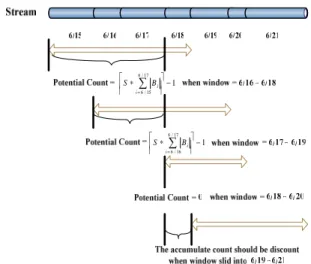
Take Figure 12 as an example. Let W be 3. Assume that an itemset g is inserted into PFP in 6/18. By Formula (1), g.Pcount is computed from the support count thresholds in 6/15-6/17. When the TS moves to 6/19, g.Pcount is decreased and only considers 6/16-6/17. As the TS moves to 6/20, since g.Acount accumulates the support counts in 6/18-6/20, g.Pcount is set 0. As the
TS moves to 6/21, g.Acount is discounted by dropping its support count in 6/18.
1 17 / 6 15 / 6 − ⎥ ⎥ ⎤ ⎢ ⎢ ⎡ ∗∑ = i i B S 1 17 / 6 16 / 6 − ⎥ ⎥ ⎤ ⎢ ⎢ ⎡ ∗∑ = i i B S
Figure 12: An example of Itemset discounting As mentioned before, PFP keeps not only the frequent itemsets in TSi but also the ones in Bi. In Formula (1), Pcount in PFP is overestimated. Therefore, if all the itemsets in PFP are outputted, it guarantees that no true answer is missed. It is called the no-false-dismissal mode (denoted as NFD). In this mode, an itemset that is frequent in Bi but not in TSi is still outputted. Sometimes user hopes that all the itemsets outputted are real answers. Therefore, we also provide the no-false-alarm mode (denoted as NFA), which outputs only the itemsets with Acount satisfying the support count threshold. Since Acount accumulates the support counts of an itemset in the individual basic blocks after that itemset is inserted into PFP, this mode guarantees that no false answer is outputted. The steps of Frequent_itemset_output are shown in Figure 13.
Input: PFP
Output: The set of frequent itemsets O
1. If (M = NFD)
For each itemset f in PFP O = O + {f}
2. Else //M=NFA
For each itemset f in PFP
If (f.Acount ≥ θ×∑i) O = O + {f} Figure 13: Frequent_itemset_output
Example 2.2
Let θ, |W|, and P be 0.4, 3, and 1 hour, respectively. Consider the stream of transactions shown in Table 1.
Table 1: A stream of transactions Time period Number of
transactions
Itemset (and its count)
B1 09:00~09:59 27 a(11),b(20),c(2),ab(6) B2 10:00~10:59 20 a(20),c(13),ac(13) B3 11:00~11:59 27 a(19),b(8),c(7),ac(7) B4 12:00~12:59 23 a(10),c(3),d(10)
Initially, PFP and DT are empty and TA[j] = 0 for all j. For the 1st hour (i.e., B1), the support count threshold is 0.4×27 (10.8). By New_itemset_insertion, only a and b are frequent and inserted into PFP with Pcount 0. In DT_maintenance, both of them are put in DT. TA is updated and the results are shown in Figure 14, where a and b are outputted for both modes.
Figure 14: A snapshot after B1 passes
For the 2nd hour (B2), the support count threshold is 0.4×20 (8). The itemsets c and ac are inserted into PFP with Pcount 10, which is the maximum possible count of a non-frequent itemset in B1. In addition, we accumulate the support counts of a in 2 hours to get its Acount (=31). In Old_itemset_update, B2 is scanned once to compute the support count of b since b is in PFP but not frequent in B2. Because the support count threshold is the sum of 10.8 and 8, i.e., 18.8, b is still kept in PFP. Finally, all the 4 itemsets are appended to DT and then TA is updated. The results are shown in Figure 15. Under the NFD mode, all the itemsets in PFP are outputted, while only a and b are outputted under the NFA mode.
Figure 15: A snapshot after B2 passes
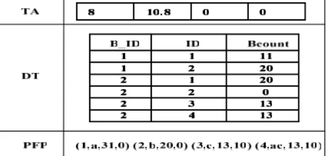
For the 3rd hour (B3), the support count threshold is also 10.8. Since the frequent itemset a in B3 also exists in PFP, we accumulate its support counts in 3 hours to get its Acount 50. In Old_itemset_update, B3 is scanned thrice to compute the support counts of b, c, and ac, respectively. For the support count threshold 29.6, we keep c and ac in PFP but delete b since its Acount plus its Pcount is 28. All the 3 itemsets are appended to DT and TA is updated. Figure 16 shows the results and only a is outputted for the NFA mode.
For the 4th hour (B4), Itemset_discounting is executed. First, we check and discount the itemsets in PFP. Since a.Pcount is 0, we decrease a.Acount as 39 according to DT. For c and ac, we first subtract TA[4] (=0) from their potential counts and then set them to 0 because they are smaller than the support count
threshold of B1. Secondly, all the entries of B1 in DT are removed. After that, we repeat the remaining operations as described above. The support count threshold of B4 is 9.2. Therefore, d is inserted into PFP with Pcount 29, while a.Acount is increased as 49. During Old_itemset_update, for c and ac, their sums of Acount and Pcount are 23 and 20, respectively. Both of them are deleted because the current support count threshold is 28 (8+10.8+9.2). The final results are shown in Figure 17.
Figure 16: A snapshot after B3 passes
Figure 17: A snapshot after B4 passes
3. Self-adjusting Discounting Table
In this section, we refine DT_maintenance to address the issue of the limited memory space. Among the data structures maintained for mining and discounting in our approach, DT often consumes most of the memory space. When the limit is reached, an efficient way to reduce the DT size without losing too much accuracy is required. A straightforward way is to merge the entries in DT as needed. The main challenge is how to quickly select the entries for merging such that the resultant DT still performs well in discounting. In the following, a naive solution called the naïve adjustment is introduced first and then our proposed method named the selective adjustment is presented.
3.1 Naïve adjustment
Since each entry is appended to the end of DT when it shows up, we can regard DT as a list of triples (B_ID,
ID, Bcount) sorted by B_ID and ID, e.g., the figures in Example 2.2. Let the kth entry in DT be DTk. Every two
adjacent entries satisfy one of the following properties: 1. DTk.B_ID < DTk+1.B_ID
2. DTk.B_ID = DTk+1.B_ID and DTk.ID < DTk+1.ID When the size of DT reaches its limit, the naïve adjustment finds the two adjacent entries satisfying the 2nd property and then merges them into one. Figure 18 illustrates the DT_maintenance with naïve adjustment, where DT_size and DT_limit respectively denote the number of entries in DT and its upper bound due to the limited memory space.
Input: PFP, DT, DT_size, DT_limit //DT_limit > |W| Output: updated DT
1. For each itemset f in PFP
1.1 If (DT_size = DT_limit) //DT is full 1.1.1 k = 2 //naïve adjustment 1.1.2 While (DTk.B_ID≠DTk-1.B_ID) k++ 1.1.3 DTk-1.ID = DTk-1.ID ∪ DTk.ID
1.1.4 If (M=NFD)
DTk-1.Bcount=min{DTk-1.Bcount, DTk.Bcount}
1.1.5 Else //M=NFA
DTk-1.Bcount=max{DTk-1.Bcount, DTk.Bcount} 1.1.6 Remove DTk from DT; DT_size--
1.2 Append f to DT; DT_size++ Figure 18: DT_maintenance with naïve adjustment
At the beginning of naïve adjustment, we scan DT from top to bottom and merge the first two entries having the same B_ID. Note that after Step 1.1.2, the entries DTk-1 and DTk always exist so long as DT_limit is larger than |W|. In this way, only the adjacent entries having the same B_ID are merged. The memory space freed is immediately used for the new entry appended to DT. Except for the unchanged B_ID, we also assign ID and Bcount to the new entry after merging. Since we sort the entries having the same B_ID by ID, the ID’s from the adjacent entries can be represented as a range of ID’s, i.e., “smallest ID−largest ID”. Therefore, as Step 1.1.3 indicates, we use the range covered by the ID’s from DTk-1 and DTk as the ID of the new DTk-1.
On the other hand, the assignment of Bcount is different and depends on the output mode M given by the user. For the NFD mode, we underestimate Bcount such that the support count of an itemset is discounted as less as possible and thus overestimated. In this case, we choose the smaller Bcount between DTk-1 and DTk as the Bcount of the new DTk-1 as Step 1.1.4 indicates. By contrast, for the NFA mode, we underestimate the support count of an itemset by discounting it as more as possible. Therefore, in Step 1.1.5, the larger Bcount between DTk-1 and DTk is chosen.
Example 3.1
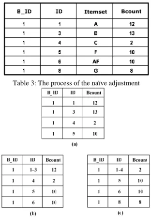
Suppose that the 6 itemsets in Table 2 will be inserted into DT but DT_limit is set to 4. In addition, the output mode is NFD. Initially, DT is empty. The 4 itemsets A,
B, C, and F are added one by one to form Table 3(a). Since DT is full now, the naïve adjustment is executed before the addition of AF. Specifically, the entries (1, 1, 12) and (1, 3, 13) are selected and merged into (1, 1−3, 12) as Table 3(b) shows. After that, AF is added to DT. For the addition of G, the naïve adjustment is executed again and the first 2 entries are merged into (1, 1−4, 2) as Table 3(c) indicates.
Table 2: The itemsets to be inserted
Table 3: The process of the naïve adjustment
The naïve adjustment is fast but provides inaccurate information for discounting when too many entries are merged together. Take (1, 1−4, 2) in Table 3(c) as an example. Due to the NFD mode, the value 2 stands for the minimum Bcount among the merged entries. When discounting itemsets A, B, and C, the errors are 10, 11, and 0, respectively. We call the sum of these errors the merging loss. For an entry in DT, the smaller merging loss it has, the more accurate Bcount it will provide for discounting. Next, we will introduce our method that uses the merging loss to select the entries for merging.
3.2 Selective Adjustment
In our method, each entry DTk is in the new form of (B_ID, ID, Bcount, AVG, NUM, Loss). DTk.AVG keeps
the average of support counts for all the itemsets merged into DTk, DTk.NUM is the number of itemsets
in DTk, while DTk.Loss records the merging loss of
merging DTk with DTk-1. The main idea of our method is to select the entry with the smallest merging loss,
called the victim, and merge it into the entry above it. DT1.Loss and DTk.Loss are set ∞ to avoid being the victim, ∀k, DTk.B_ID≠DTk-1.B_ID. Since the merging loss of an entry depends on the output mode M, we formulate it as follows:
Definition 3.1 Merging loss
For k>1 and DTk.B_ID=DTk-1.B_ID, DTk.Loss under the NFD mode is computed as follows:
( )
{DT.Bcount,DT .Bcount} (DT.NUM DT .NUM) (2)
min .AVG DT .NUM DT .AVG DT .NUM DT 1 -k k 1 -k k 1 -k 1 -k k k + × − × + ×
DTk.Loss under the NFA mode is computed as follows:
{ } ( )
(DT.NUM DT.AVG DT .NUM DT .AVG) (3)
.NUM DT .NUM DT .Bcount DT .Bcount, DT max 1 -k 1 -k k k 1 -k k 1 -k k × + × − + ×
According to the same reason for the assignment of Bcount in the naïve adjustment, we use the minimum (maximum) Bcount in the computation of merging loss under the NFD (NFA) mode. As a result, the smaller merging loss DTk has, after merging, the more accurate Bcount DTk-1 will provide. Figure 19 illustrates the DT_maintenance with selective adjustment.
Input: PFP, DT, DT_size, DT_limit Output: updated DT
1. For each itemset f in PFP 1.1 If (DT_size = DT_limit)
1.1.1 Scan DT once to select the victim //DTk
1.1.2 DTk-1.ID = DTk-1.ID ∪ DTk.ID 1.1.3 If (M=NFD)
DTk-1.Bcount=min{DTk-1.Bcount, DTk.Bcount}
1.1.4 Else //M=NFA
DTk-1.Bcount=max{DTk-1.Bcount, DTk.Bcount} 1.1.5 DTk-1.NUM = DTk-1.NUM + DTk.NUM 1.1.6 Compute DTk-1.AVG
1.1.7 If (DTk-1.Loss≠∞) Recalculate DTk-1.Loss 1.1.8 Remove DTk from DT; DT_size-- 1.1.9 If (DTk+1.Loss≠∞) Recalculate DTk+1.Loss 1.2 Append f to DT; DT_size++
Figure 19: DT_maintenance with selective adjustment At the beginning of selective adjustment, we scan DT once to find the victim. Suppose that DTk is the victim and will be merged into DTk-1. For the new DTk-1, the assignment of ID and Bcount follows the same way in the naïve adjustment. Moreover, NUM is assigned with the sum of DTk-1.NUM and DTk.NUM, while AVG is computed as follows:
) 4 ( .NUM 1 k DT .NUM k DT .NUM 1 -k DT .AVG 1 -k DT .NUM k DT .AVG k DT − + × + ×
Based on the new DTk-1.Bcount, DTk-1.AVG, and DTk-1.NUM, DTk-1.Loss can be computed by Definition 3.1. Note that if the old DTk-1.Loss has been set ∞, it is unchanged. After the merging, the merging loss of the entry below the victim, i.e., DTk+1.Loss, is also updated as Step 1.1.9 indicates.
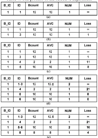
Example 3.2
Consider Table 2, DT_limit=4, and M=NFD. Table 4(a) shows the DT as itemset A is added. Since it is the first entry, its merging loss is set ∞. As itemset B is added, we compute its merging loss by Formula (2) and the result is shown in Table 4(b). In the same way, we add itemsets C and F to form the DT in Table 4(c). Since DT is full now, the selective adjustment is executed before the addition of AF. Specifically, the entry (1, 3, 13, 13, 1, 1) is selected as the victim and merged with (1, 1, 12, 12, 1, ∞). The result after merging forms the first entry in Table 4(d), where DT1.Loss is ∞ and DT1.AVG (=12.5) is computed by Formula (4). Notice that DT2.Loss is changed from 11 to 21 as Step 1.1.9 indicates. Finally, we add itemset G in a similar way to obtain the final result in Table 4(e).
Table 4: The process of the selective adjustment
Consider the final results in Example 3.1 and 3.2. In the former, the sum of all the merging losses is (12-2) + (13-2) + (2-2) + (10-10) + (10-10) + (8-8) = 21. In the latter, the sum of all the merging losses is (12-12) + (13-12) + (2-2) + (10-10) + (10-10) + (8-8) = 1. In this case, obviously, our method provides a higher accuracy of discounting information than a naïve solution.
4. Experiments
In this section, we will describe the experimental evaluation of our algorithms. The experimental setting
is first described and then the results are presented.
4.1 Experimental Setting
The experiments are made upon the PC with the Intel Pentium-M 1.3GHz CPU, 256 MB main memory and Microsoft Windows XP Professional. The programs are written in C and compiled using Microsoft Visual C++ 6.0. The mining algorithm we applied to find frequent itemsets in a basic block is the FP-growth. The datasets streaming into our system are synthesized via the IBM data generator [2], where we adopt most of its default values for the command options. For clarity, we name each dataset in the form of TxxIxxDxx, where T, I, and D mean the average transaction length, the average length of the maximum pattern, and the total number of transactions, respectively. To simulate data streams, we divide a dataset into basic blocks with equal size (i.e., 10K transactions) and feed them into the buffer. The parameter setting used in the experiments (unless explicitly specified otherwise) is shown in Table 5.
Table 5: Parameter setting
Parameter Value
Number of distinct items 1K
DT_limit 10K θ 0.0025 |W| 4 T 3~7 I 4 D 150K
Two kinds of experiments have been made. First, the required execution time and memory usage are two indicators of the efficiency for mining data streams. We compare the execution times of our approach in the PFP maintenance part, the DT maintenance part, and the mining part (FP-growth). The memory usage referring to the memory space consumed for both PFP and DT is reported. In addition, the scalability of our approach for the minimum support threshold is also evaluated. On the other hand, under the NFD (NFA) mode, the number of false alarms (false dismissals) is also a good indicator of the effectiveness for mining data streams. We define measures to estimate them and to compare the two strategies for maintaining the SDT.
4.2 Efficiency on Time and Space
First, we evaluate the execution time of our approach adopting the selective adjustment for T=3~7. Since the results show similar trends, only Figure 20 (T=7) is shown. The 4 curves in it refer to the execution time in 3 parts and the total, respectively. Our observations are as follows:
• The mining part dominates the total execution time. That is, New_itemset_insertion is the bottleneck of our algorithm, while the other operations are fast.
• The execution time of DT maintenance part is close
to zero in most cases. It verifies the feasibility of the SDT for mining data streams.
• Although the execution time of the mining part is sensitive to T, the total execution time increases slowly as the growth of T. It indicates the fast response time our approach achieved.
0 6 12 18 24 30 36 42 1 2 3 4 5 6 7 8 9 10 11 12 13 14 15
Basic block number
E x ec u tio n tim e (S ec on d) Total PFP maintenance part DT maintenance part Mining
Figure 20: Execution time for T = 7
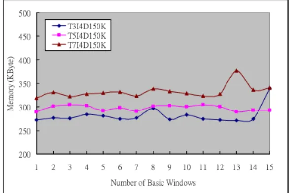
Figure 21 shows the memory usage under different values of T. The highest peak of memory usage during the experiment is not more than 350KB. It verifies the feasibility of the SDT, especially for the streaming environment with only a small memory. In all the figures, the curves are near smooth when the data stream flows. It implies that our approach adapts itself very well no matter how long a data stream is.
200 250 300 350 400 450 500 1 2 3 4 5 6 7 8 9 10 11 12 13 14 15
Number of Basic Windows
Me m o ry ( K B yt e) T3I4D150K T5I4D150K T7I4D150K
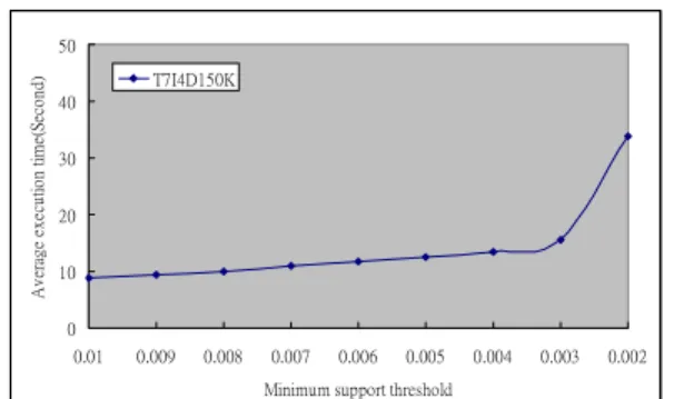
Figure 21: Memory usage for T = 3, 5, 7 To evaluate the scalability of our approach, we try
θ=0.01~0.002 on the data set T7I4D150K. Intuitively,
a smaller θ implies more frequent itemsets, indicating a higher execution time. As expected, in Figure 22, the average execution time grows slowly as the decreases of θ, but the curve has a sharp rise when θ is changed from 0.003 to 0.002. We found that the number of frequent itemsets for θ=0.002 is six times as many as the case for θ=0.003. Therefore, our approach can be stable as long as the number of frequent itemsets does not increase very dramatically.
0 10 20 30 40 50 0.01 0.009 0.008 0.007 0.006 0.005 0.004 0.003 0.002 Minimum support threshold
A v er ag e ex ecu ti o n ti m e( S eco n d) T7I4D150K
Figure 22: Average execution time for θ = 0.01~0.002
4.3 Effectiveness on NFD and NFA
To evaluate the effectiveness of the proposed strategies for maintaining the SDT, we make an experiment on the data set T7I4D150K, where the DT_limit is varied from 4 to 12K. The experiment is performed for the NFD and NFA modes, respectively.
Under the NFD mode, we overestimate the support count of each itemset in PFP. Therefore, it guarantees no false dismissal but allows false alarms. Intuitively, the smaller the DT_limit is, the more adjustments and false alarms will occur. In our setting, the case when DT_limit=4 is the worse case, while the case when DT_limit=12K is the best case. We define a measure to evaluate the effectiveness under the NFD mode:
Definition 4.1 False Alarm Rate
The false alarm rate when DT_limit=M (denoted as FARM) can be computed as follows:
) 5 ( case the worst in alarms false of number The M it DT when alarms false of number The FARM lim _ = =
The results are shown in Figure 23, where the false alarm rate shrinks as the growth of DT_limit. Consider the selective adjustment. 40% reduction of FAR is achieved when DT_limit=2K. As DT_limit=6K, more than 80% reduction of FAR can be achieved. From the two curves, it is obvious that the selective adjustment outperforms the naïve adjustment.
0 20 40 60 80 100 4 1000 2000 3000 4000 5000 6000 7000 8000 9000 10000 11000 12000 DT_limit FA R ( % ) Selective adjustment Naive adjustment
Figure 23: False alarm rate under the NFD mode On the contrary, we underestimate the support count of each itemset in PFP under the NFA mode. Therefore, it guarantees no false alarm but allows false dismissals. A smaller DT_limit implies more false dismissals. The
worse case and the best case are the same as described above. Similarly, we define a measure to evaluate the effectiveness under the NFA mode:
Definition 4.2 False Dismissal Rate
The false dismissal rate when DT_limit=M (denoted as FDRM) can be computed as follows:
) 6 ( case the worst in dismissals false of number The M it DT when dismissals false of number The FDRM lim _ = =
The results shown in Figure 24 also indicate that the false dismissal rate shrinks as the growth of DT_limit. The selective adjustment again outperforms the naïve adjustment. For example, the selective adjustment can achieve 60% reduction of FDR as DT_limit=4K, while the naïve adjustment cannot make it until DT_limit=9K. Our approach is both efficient and effective since it works well in the environment with a small memory and achieves fast response time without producing too many false alarms or false dismissals.
0 20 40 60 80 100 4 1000 2000 3000 4000 5000 6000 7000 8000 9000 10000 11000 12000 DT_limit FDR (% ) Selective adjustment Naive adjustment
Figure 24: False dismissal rate under the NFA mode
5. Conclusion
Mining data streams is an interesting and challenging research field. The characteristics of data streams make the traditional mining algorithm unable to be applied. In this paper, we introduce an efficient algorithm for mining frequent itemsets over data streams under the time-sensitive sliding-window model. We design the data structures for mining and discounting the support counts of the frequent itemsets when the window slides. Moreover, two strategies for keeping SDT for the limited memory are proposed. Finally, the experiment results demonstrate that the execution time and required memory of our approach are acceptable under various parameter settings. On the other hand, the SDT performs well when the available memory is limited.
From this study, more topics are uncovered. First, we provide either of the two accuracy guarantees for the frequent itemsets found in this paper. However, the errors in the support counts are not precisely estimated or bounded. The error estimation can help the ranking of frequent itemsets if only the top-k frequent itemsets are needed. Second, any other type of frequent patterns such as the sequential pattern can be the next target. Finally, the constraints recently discussed in the data mining field can also be included into this study.
Acknowledgement
This work is partially supported by the National Science Council of the Republic of China under Grant No. 93-2752-E-007-004-PAE.
Reference
[1] D.J. Abadi, D. Carney, U. Cetintemel, et al., “Aurora: A New Model and Architecture for Data Stream Management,” The VLDB Journal, 12(2): 120-139, 2003.
[2] R. Agrawal and R. Srikant, “Fast Algorithms for Mining Association Rules,” Proc. of VLDB Conf., pp. 487-499, 1994.
[3] A. Arasu and G.S. Manku, “Approximate Counts and Quantiles over Sliding Windows,” Proc. of ACM PODS Symp., 2004.
[4] B. Babcock, S. Babu, M. Datar, R. Motwani, and J. Widom, “Models and Issues in Data Stream Systems,” Proc. of ACM PODS Symp., 2002.
[5] B. Babcock, M. Datar, R. Motwani, and L. O’Callaghan, “Maintaining Variance and k–Medians over Data Stream Windows,” Proc. of ACM PODS Symp., 2003.
[6] S. Chandrasekaran, O. Cooper, A. Deshpande, M.J. Franklin, et al., “TelegraphCQ: Continuous Dataflow Processing for an Uncertain World,” The First Conf. on Innovative Data Systems Research (CIDR), 2003.
[7] J.H. Chang and W.S. Lee, “Finding Recent Frequent Itemsets Adaptively over Online Data Streams,” Proc. of ACM SIGKDD Conf., pp. 487-492, 2003.
[8] C.H. Chang and S.H. Yang, “Enhancing SWF for Incremental Association Mining by Itemset Maintenance,” Proc. of Pacific-Asia Conf. on Knowledge Discovery and Data Mining, 2003.
[9] M. Charikar, K. Chen, and M. Farach-Colton, “Finding Frequent Items in Data Streams,” Proc. of Inter’l Colloquium on Automata, Languages and Programming (ICALP), pp. 693-703, 2002.
[10] M. Charikar, L. O’Callaghan, and R. Panigrahy, “Better Streaming Algorithms for Clustering Problems,” Proc. of ACM Symp. on Theory of Computing (STOC), pp. 30-39, 2003.
[11] J. Chen, D.J. DeWitt, F. Tian, and Y. Wang, “NiagaraCQ: A Scalable Continuous Query System for Internet Databases,” Proc. of ACM SIGMOD Conf., pp. 379-390, 2000.
[12] D. Cheung, J. Han, V. Ng, and C.Y. Wong, “Maintenance of Discovered Association Rules in Large Databases: An Incremental Updating Technique,” Proc. of ICDE Conf., 1996.
[13] E. Cohen and M. Strauss, “Maintaining Time Decaying Stream Aggregates,” Proc. of ACM PODS Symp., 2003.
[14] G. Cormode and S. Muthukrishnan, “What's Hot and What's Not: Tracking Most Frequent Items Dynamically,” Proc. of ACM PODS Symp., pp. 296-306, 2003.
[15] E. Demaine, A. Lopez-Ortiz, and J.I. Munro, “Frequency Estimation of Internet Packet Streams with Limited Space,” Proc. of European Symp. on Algorithms (ESA), pp. 348-360, 2002.
[16] C. Giannella, J. Han, J. Pei, X. Yan, and P.S. Yu, “Mining Frequent Patterns in Data Streams at Multiple Time Granularities,” H. Kargupta, A. Joshi, K. Sivakumar, and Y. Yesha (eds.), Next Generation Data Mining, pp. 191-212, 2003.
[17] L. Golab and M. Ozsu, “Issues in Data Stream Management,” ACM SIGMOD Record, 32(2): 5-14, 2003.
[18] J. Han, J. Pei, Y. Yin, and R. Mao, “Mining Frequent Patterns without Candidate Generation: A Frequent-Pattern Tree Approach,” Data Mining and Knowledge Discovery, 8(1): 53-87, Kluwer Academic Publishers, 2004.
[19] G. Hulten, L. Spencer, and P. Domingos, “Mining Time Changing Data Streams,” Proc. of ACM CIKM Conf., pp. 97-106, 2001.
[20] C. Jin, W. Qian, C. Sha, J.X. Yu, and A. Zhou, “Dynamically Maintaining Frequent Items over a Data Stream,” Proc. of ACM CIKM Conf., 2003.
[21] R.M. Karp, C.H. Papadimitriou, and S. Shenker, “A Simple Algorithm for Finding Frequent Elements in Streams and Bags,” ACM Trans. on Database Systems (TODS), 28(1): 51-55, 2003.
[22] C. Lee, C. Lin, and M. Chen, “Sliding-window Filtering: An Efficient Algorithm for Incremental Mining,” Proc. of ACM CIKM Conf., 2001.
[23] J. Liu, Y. Pan, K. Wang, and J. Han, “Mining Frequent Item Sets by Opportunistic Projection,” Proc. of ACM SIGKDD Conf., 2002.
[24] G. Manku and R. Motwani, “Approximate Frequency Counts over Data Streams,” Proc. of VLDB Conf., pp. 346-357, 2002.
[25] R. Motwani, J. Widom, A. Arasu, and B. Babcock, “Query Processing, Approximation, and Resource Management in a Data Stream Management System,” CIDR Conf., 2003.
[26] L. O’Callaghan, N. Mishra, A. Meyerson, S. Guha, and R. Motwani, “Streaming-Data Algorithms for High-Quality Clustering,” Proc. of ICDE, pp. 685-696, 2002.
[27] W. Teng, M.S. Chen and P. Yu, “A Regression-Based Temporal Pattern Mining Scheme for Data Streams,” Proc. of VLDB Conf., pp.93-104, 2003.
[28] Y. Zhu and D. Shasha, “StatStream: Statistical Monitoring of Thousands of Data Streams in Real Time,” Proc. of VLDB Conf., 2002.