Collocation Methods for Poisson’s Equation
Hsin-Yun Hu∗, and Zi-Cai Li†January 31, 2005
Abstract
In this paper, we provide an analysis on the collocation methods(CM), which uses a large scale of admissible functions such as orthogonal polynomials, trigonometric functions, radial basis functions and particular solutions, etc. The admissible functions can be chosen to be piecewise, i.e., different functions are used in different subdomains. The key idea is that the collocation method can be regarded as the least squares method involving integration approximation, and optimal convergence rates can be easily achieved based on the tradi-tional analysis of the finite element method. The key analysis is to prove the uniformly Vh− elliptic inequality and some inverse inequalities used. This paper explores the interesting fact that the integration rules only affect on the uniformly Vh− elliptic inequality, but not on the solution accuracy. The advantage of the CM is to formulate easily the associated algebraic equations, which can be solved from the collocation equations directly by the least squares method, thus to greatly reduce the condition number of the associated matrix. Note that the boundary approximation method in Li [13] is a special case of the CM, where the admissible functions satisfy the equations exactly. Numerical experiments are also carried for Poisson’s problem to support the analysis made.
keywords: Collocation method, least squares method, Poisson’s equation, Error analysis, Motz’s problem.
AMS Subject classification, 65N10, 65N30.
1
Introduction
If the admissible functions are chosen to be analytical functions, e.g., trigonometric al or other orthogonal functions, we may enforce them to satisfy directly the PDE at certain collocation points, by letting the residuals to be zero. This leads to the collocation method(CM). The CM
∗National Center for Theoretical Sciences Mathematics Division, National Tsing Hua University, Hsinchu,
Taiwan 30043
†Corresponding author, E-mail: [email protected], Department of Applied Mathematics, National Sun
is a popular method in engineering computation, because the algebraic equations can be easily formulated. For CM method, there are many reference books, see in Bernardi and Maday [4], Canuto et al. [6], Gottlieb and Orszag [11], Quarteroni and Valli [19] and Mercier [17]. There have been several important studies of CM: Bernardi et al. [3], Shen [20, 21, 22], Arnold and Wendland [1], Canuto et al. [5], Pathria and Karniadakis [18], and Sneddon [23].
In this paper, we present a new analysis of CM by following the ideas in Li [13] that other numerical methods can be regarded as a special kind of the Ritz-Galerkin method. The CM is, indeed, the least squares method, which is treated as the Ritz-Galerkin method, involving integration approximation. The advantages of the CM are twofold: (1) flexibility of applica-tion to different geometric shapes and different elliptic equaapplica-tions, (2) simplicity of computer programming. The optimal error bounds can be easily derived, based on the uniformly Vh−
elliptic inequality, which is proved in detail in this paper.
This paper is organized as follows. In the next section, the collocation method with an interior boundary is described, and in Section 3 an analysis is given. In Section 4 the CM for the Robin boundary conditions is discussed, and in Section 5, some inverse inequalities are provided. In the last section, the numerical experiments including singularity problems are carried out to support the analysis made.
2
Description of Collocation Methods
Consider the Poisson’s equation on domain S with the mixed type of the Dirichlet and Neumann conditions, − 4 u = − Ã ∂2u ∂x2 + ∂2u ∂y2 ! = f (x, y) in S, (2.1) u|ΓD = g1 on ΓD, (2.2) uν|ΓN = g2 on ΓN, (2.3)
where S is a polygon, ∂S = Γ = ΓD∪ΓN is its boundary, uν = ∂u∂ν, and ν is the outnormal to ∂S.
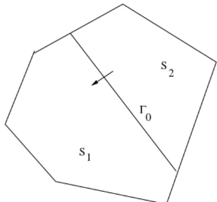
Let S be divided by Γ0 into two disjoint subregions, S1 and S2 (see Figure 1): S = S1∪ S2∪ Γ0
and S1∩ S2 = ∅. We give a few assumptions.
A1: The solutions in S1 and S2 can be expanded as
v = v−= ∞ X i,j=1 aijΦi(x)Φj(y) in S1, v+= X∞ i,j=1 bijΨi(x)Ψj(y) in S2, (2.4)
where {Φi(x)Φj(y)} and {Ψi(x)Ψj(y)} are complete and independent bases in S1 and S2
A2: The basis functions
Φi(x)Φj(y) ∈ C2(S1) ∩ C1(∂S1), Ψi(x)Ψj(y) ∈ C2(S2) ∩ C1(∂S2). (2.5)
A3: The expansions in (2.4) converge exponentially to the true solutions u±,
u−= u−m+ Rm−, u+= u+n + R+n, (2.6) where u− = u¯¯¯ S1 and u+= u¯¯¯ S2 , and u−m= m X i,j=1 aijΦi(x)Φj(y), u+n = n X i,j=1 bijΨi(x)Ψj(y), (2.7) R−
m and R+n are the remainders, and aij and bij are the true expansion coefficients. Then
max S1 |R−m| = O(e−¯cm), max S2 |R+n| = O(e−¯cn), (2.8) where ¯c > 0, m > 1 and n > 1.
Based on A1-A3 we may choose the piecewise admissible functions,
v = v−= m X i,j=1 ˜aijΦi(x)Φj(y) in S1, v+= Xn i,j=1 ˜bijΨi(x)Ψj(y) in S2, (2.9)
where ˜aij and ˜bij are unknown coefficients to be sought. Since v on Γ0 are not continuous, v±
have to satisfy the interior continuity conditions
u+= u−, u+ν = u−ν, on Γ0, (2.10) where uν = ∂u∂ν, and ν is the outward unit normal of ∂S2.
Based on A2 we may seek the coefficients ˜aij and ˜bij by satisfying (2.1)-(2.3) and (2.10)
directly at nodes Qij and Qi,
(∆v±+ f )(Q±ij) = 0, Q±ij ∈ S±, (2.11) (v − g1)(Qi) = 0, Qi∈ ΓD, (2.12)
(vν− g2)(Qi) = 0, Qi ∈ ΓN, (2.13)
(v+− v−)(Qi) = 0, Qi∈ Γ0, (2.14)
(vν+− vν−)(Qi) = 0, Qi∈ Γ0, (2.15) where v± also denotes v±¯¯¯
Γ0
, S− = S
1, and S+ = S2. Eqs. (2.11)–(2.15) can be written in a
matrix form
where ~x is the unknown vector consisting of ˜aij and ˜bij, ~b is the known vector, and F ∈
RM ×(m2+n2), where M (≥ m2+ n2) is the total number of all collocation nodes Q±ij ∈ S±, and
Qi∈ ΓD∪ ΓN∪ Γ0. In this paper, we always choose M > (m2+ n2) and even M >> (m2+ n2).
Consequently, we obtain an overdetermined system which can be solved by the least square method (i,.e., the QR decomposition or the singular value decomposition), see Golub and Loan [10].
Below, let us view the CM as the least squares method involving integration approximation. Denote by Vh the finite dimensional collection of the admissible functions (2.9). We given one more assumption.
A4: Suppose that there exists a positive constant µ(> 0) such that
kvν±k0,ΓD∩S± ≤ CLµkv±k1,S±, v ∈ Vh, (2.17) kvν+k0,Γ0∩S+ ≤ CLµkv+k1,S+, v ∈ Vh. (2.18)
For polynomials of order L, we will prove (2.17) and (2.18) with µ = 2 in Section 5. Then the approximate coefficients ˜aij and ˜bij can be obtained by the least squares methods: To seek the
approximation solution um,n ∈ Vh such that
E(um,n) = min v∈Vh E(v), (2.19) where E(v) =1 2{ Z Z S1 (∆v−+ f )2+ Z Z S2 (∆v++ f )2 (2.20) +L2µ Z Γ0 (v+− v−)2+ Z Γ0 (v+ν − v−ν)2 +L2µ Z ΓD (v − g1)2+ Z ΓN (vν− g2)2}.
Eq. (2.20) can be described equivalently
a(um,n, v) = f (v), ∀v ∈ Vh, (2.21) where a(u, v) = Z Z S1 ∆u∆v + Z Z S2 ∆u∆v (2.22) +L2µ Z Γ0 (u+− u−)(v+− v−) + Z Γ0 (u+ν − u−ν)(vν+− vν−) +L2µ Z ΓD uv + Z ΓN uνvν, f (v) = − Z Z S1 f ∆v − Z Z S2 f ∆v + L2µ Z ΓD g1v + Z ΓN g2vν, (2.23)
The integrals in (2.22) can be approximated by some rules of integration: d Z Z S±g = X ij α±ijg(Q±ij), Q±ij ∈ S±, (2.24) c Z Γ0 g =X i αig(Qi), Qi∈ Γ0, c Z ΓD g =X i αDi g(Qi), Qi∈ ΓD, c Z ΓN g =X i αNi g(Qi), Qi∈ ΓN,
where α±ij, αi, αDi and αNi are positive weights, and Q±ij and Qi are integration nodes. The least
squares method (2.21) is then reduced to
ˆa(ˆum,n, v) = ˆf (v), ∀v ∈ Vh, (2.25) where ˆa(u, v) = d Z Z S1 ∆u∆v + d Z Z S2 ∆u∆v (2.26) +L2µc Z Γ0 (u+− u−)(v+− v−) +c Z Γ0 (u+ν − u−ν)(v+ν − v−ν) +L2µc Z ΓD uv +c Z ΓN uνvν, ˆ f (v) = −d Z Z S1 f ∆v − d Z Z S2 f ∆v + L2µc Z ΓD g1v + c Z ΓN g2vν. (2.27)
It is easy to see that by the rules (2.24), the following algebraic equations can be obtained from (2.25) directly, q α±ij(∆v±+ f )(Q±ij) = 0, Q±ij ∈ S±, (2.28) √ αiLµ(v+− v−)(Qi) = 0, Qi ∈ Γ0, (2.29) √ αi(vν+− vν−)(Qi) = 0, Qi∈ Γ0, (2.30) q αD i Lµ(v − g1)(Qi) = 0, Qi ∈ ΓD, (2.31) q αN i (vν − g2)(Qi) = 0, Qi ∈ ΓN. (2.32)
Compared with (2.11)–(2.15), Eqs. (2.28)–(3.32) can be denoted by
WF~x = W~b, (2.33)
where F is given in (2.16), and W ∈ RM ×M is the diagonal weight matrix, consisting of the
weights, qα±ij, Lµ√α i, √αi, Lµ q αD i and q αN
by solving the normal equation:
A~x = ~b∗, (2.34)
where matrix A = FTWTWF is symmetric and positive definite, and the known vector ~b∗ =
FTWTW~b. In real computation, when M > (m2+ n2), we always solve (2.33) directly by the
least squares method using the QR method1, and the condition number is defined in [10] by
Cond. = ½ λmax(A) λmin(A) ¾1 2 , (2.35)
where λmax(A) and λmin(A) are the maximal and minimal eigenvalues, respectively. Note that
Eq. (2.35) is square root of the condition number by solving the normal equations.
3
Error Analysis
We will provide the error bounds for the solutions from (2.21)–(2.25). Denote the the space
H∗= {v, v ∈ L2(S), v±∈ H1(S±), ∆v±∈ L2(S±)}, (3.1) accompanied with the norm
kvkH = {kvk21+ k∆vk20,S1 + k∆vk 2 0,S2+ L 2µkv+− v−k2 0,Γ0 (3.2) + kvν+− vν−k20,Γ0+ L2µkvk20,ΓD + kvνk20,ΓN} 1/2, where kvk1= {kvk21,S1 + kvk 2 1,S2} 1 2, |v|1= {|v|2 1,S1 + |v| 2 1,S2} 1 2, (3.3)
and kvk1,S1, kvk0,Γ0, etc. are the Sobolev norms. Obviously, Vh ⊂ H∗. Then
kvk2H = kvk21+ a(v, v). (3.4) Now we have a theorem.
Theorem 3.1 Suppose that there exist two inequalities
a(u, v) ≤ CkukH × kvkH, ∀v ∈ Vh, (3.5)
a(v, v) ≥ C0kvk2H, ∀v ∈ Vh, (3.6)
where C0 > 0 and C are two constants independent of m and n. Then, the solution of the least squares method (2.21) has the error bound,
ku − um,nkH = C inf v∈Vh ku − vkH (3.7) ≤ ε1= kR−mk2,S1+ kRn+k2,S2 + LµkRLk0,ΓD∪Γ0+ k(RL)νk0,ΓN∪Γ0, where |RL| = |R− m| + |R+n|.
Proof : For the true solution, we have a(u, v) = f (v), ∀v ∈ Vh. Then
a(u − um,n, v) = 0, ∀v ∈ Vh. (3.8) Denote the projection solution on Vh
uI = u−I = m X i=1 aijΦi(x)Φj(y) in S1, u+I = n X i=1 bijΨi(x)Ψj(y) in S2, (3.9)
where aij and bij are the true expansion coefficients. Then uI ∈ Vh. Let v ∈ Vh, and w =
um,n− v ∈ Vh, We have from (3.6), (3.8) and (3.5)
C0kwk2H ≤ a(um,n− v, w) = a(u − v, w) (3.10) ≤ ku − vkHkwkH. This leads to kum,n− vkH = kwkH ≤ Cku − vkH. (3.11) Then we obtain kum,n− ukH ≤ kum,n− vkH + ku − vkH ≤ Cku − vkH (3.12) and kum,n− ukH ≤ C inf v∈Vh ku − vkH. (3.13) Let v = uI we have kum,n− ukH ≤ C inf v∈Vh ku − vkH ≤ Cku − uIkH (3.14) ≤ kR−mk2,S1+ kR+nk2,S2+ LµkRLk0,ΓD∪Γ0+ k(RL)νk0,ΓN∪Γ0.
This completes the proof of Theorem 3.1. .
Since the solution u in (2.1)-(2.3) satisfies the collocation equations (2.28)-(2.32) exactly, then
ˆa(u, v) = ˆf (v), ∀v ∈ Vh. (3.15) We can also prove the following theorem.
Theorem 3.2 Suppose that there exist two inequalities
ˆa(u, v) ≤ CkukH × kvkH, ∀v ∈ Vh, (3.16)
where C0 > 0 and C are two constants independent of m and n. Then, the solution of the collocation method (2.25) has the error bound,
ku − ˆum,nkH = C inf v∈Vh
ku − vkH ≤ ε1, (3.18)
where ε1 is given in (3.7).
Note that for the FEM, FDM, etc,. the true solution does not satisfy (3.15), then Theorem 3.2 may not hold. Also, the analysis in this paper is different form the traditional analysis in collocation method in [4, 6, 11, 19], where only the zeros of polynomials are used as the collocation nodes.
Below we prove the uniformly Vh− elliptic inequalities (3.6) and (3.17). We cite a lemma
from [14].
Lemma 3.1 Let ΓD∩ S−6= ∅. If v ∈ H∗, then there exists a positive constant C independent
of v such that kvk1 ≤ C © |v|1+ kvk0,ΓD+ kv +− v−k 0,Γ0 ª .
Lemma 3.2 Let A4 be given, and ΓD∩ S1 6= ∅. There exists the bound for v ∈ Vh,
C0kvk21 ≤ a(v, v), v ∈ Vh, (3.19)
where C0(> 0) is a constant independent of m and n.
Proof : We have |v|21 = Z Z S1 |∇v|2+ Z Z S2 |∇v|2 (3.20) = − Z Z S1 v∆v − Z Z S2 v∆v + Z ∂S1 v−νv−+ Z ∂S2 vν+v+ = − Z Z S1 v∆v − Z Z S2 v∆v + Z Γ0 (vν+v+− vν−v−) + Z ΓD vνv + Z ΓN vνv,
where ν is the unit outnormal to ∂S or ∂S2. Below, we give the bounds of all terms in the right
hand side in the above equation. First we have from (2.18)
| Z Γ0 (v+νv+− vν−v−)| ≤ | Z Γ0 (v+− v−)vν+| + | Z Γ0 (vν+− vν−)v−| (3.21) ≤ kv+− v−k0,Γ0kv + νk0,Γ0 + kv + ν − vν−k0,Γ0kv −k 0,Γ0 ≤ C{Lµkv+− v−k0,Γ0 + kvν+− vν−k0,Γ0}kvk1,
where we have used the bounds,
kv−k0,Γ0 ≤ kv −k
1,S−, kv±k0,S± ≤ kvk1.
Next, we obtain from (2.17) and (2.18)
| Z ΓD vνv| ≤ kvk0,ΓDkvνk0,ΓD ≤ CL µkvk 0,ΓDkvk1, (3.22) | Z ΓN vνv| ≤ kvνk0,ΓNkvk0,ΓN ≤ Ckvνk0,ΓNkvk1. (3.23)
Moreover, there exist the bounds,
| Z Z S1 v∆v| ≤ k∆vk0,S1kvk0,S1 ≤ k∆vk0,S1kvk1, (3.24) | Z Z S2 v∆v| ≤ k∆vk0,S2kvk1. (3.25) From (3.19)–(3.25), |v|21≤ {k∆vk0,S1 + k∆vk0,S2 (3.26) +CLµ(kv+− v−k0,Γ0 + kvk0,ΓD) + kvν+− vν−k0,Γ0 + kvνk0,ΓN}kvk1.
Hence we have from Lemma 3.1
kvk21 ≤ C{|v|21+ kvk20,ΓD+ kv+− v−k20,Γ0} (3.27)
≤ C{|v|21+ (kvk0,ΓD+ kv+− v−k0,Γ0)kvk1}.
Combining (3.26) and (3.27) gives
kvk21≤ C{k∆vk0,S1+ k∆vk0,S2 (3.28) +Lµ(kv+− v−k0,Γ0+ kvk0,ΓD) + kv + ν − v−νk0,Γ0 + kvνk0,ΓN}kvk1. This leads to kvk1≤ C{k∆vk0,S1+ k∆vk0,S2 (3.29) +Lµ(kv+− v−k0,Γ0+ kvk0,ΓD) + kv+ν − v−νk0,Γ0 + kvνk0,ΓN}, and then kvk21≤ C{k∆vk20,S1+ k∆vk20,S2 (3.30) +L2µ(kv+− v−k20,Γ0 + kvk20,ΓD) + kvν+− vν−k20,Γ0 + kvνk20,ΓN} ≤ Ca(v, v).
Theorem 3.3 Let A4 and ΓD ∩ ∂S1 6= ∅ hold. Then there exists the uniformly Vh− elliptic inequality (3.6).
Proof : From Lemma 3.2, we have the bound,
a(v, v) = 1 2a(v, v) + 1 2a(v, v) ≥ C0kvk 2 1+ 1 2{k∆vk 2 0,S1+ k∆vk 2 0,S2 (3.31) +L2µ(kv+− v−k20,Γ0 + kvk20,ΓD) + kv+ν − vν−k20,Γ0k + kvνk20,ΓNk} ≥ ¯C0kvk2H,
where ¯C0= min{12, C0}. This completes the proof of Theorem 3.3.
Next, we derive the uniformly Vh− elliptic inequality (3.17). We give a stronger assumption
than A4.
A5: Suppose that there exists a positive constant µ(> 0) such that for v ∈ Vh
kv±kk,ΓD∩S±≤ CLkµkv±k0,Γ D∩S±, (3.32) kv±kk,Γ0 ≤ CLkµkv±k0,Γ0, (3.33) kvν±kk,ΓN∩S± ≤ CL(k+1)µkv±k1,S±, (3.34) kvν±kk,Γ0∩S±≤ CL(k+1)µkv±k1,S±, (3.35) where k = 0, 1, ....
We will give an analysis for the integration approximation. Take RbΓ0(v+
ν − v−ν)2 as an
example. Choose the integral rule of order r,
c Z Γ0 g = Z Γ0 ˆ g, (3.36)
where ˆg is the interpolant polynomial of order r on the partition Γ0 with the maximal
meshspac-ing h. Denote
kvk20,Γ0 =c
Z Γ0
v2. (3.37)
We have the following lemma.
Lemma 3.3 Let (3.35) be given. For rule (3.36) with order r, there exists the bound for v ∈ Vh,
| kvν+− vν−k 2 0,Γ0− kv + ν − v−νk 2 0,Γ0| ≤ Ch r+1L(r+3)µkvk2 1. (3.38) Proof : Let g = (v+ ν − v−ν)2, We have | kvν+− v−νk 2 0,Γ0− kv + ν − vν−k20,Γ0| = | Z Γ0 (ˆg − g)| (3.39) ≤ Chr+1|g|r+1,Γ0,
where |g|r+1,Γ0 = |(vν+− vν−)2|r+1,Γ0 ≤ 2|(vν+)2|r+1,Γ0 + 2|(vν−)2|r+1,Γ0. (3.40) From (3.35), |(vν+)2|r+1,Γ0 ≤ C r+1X i=0 |vν+|r+1−i,Γ0|vν+|i,Γ0 (3.41) ≤ C r+1X i=0 (L(r−i+2)µkvk1,S2) × (L(i+1)µkvk1,S2) ≤ CL(r+3)µkvk21,S2. Similarly, |(v−ν)2|r+1,Γ0 = CL(r+3)µkvk21,S1. (3.42)
Combining (3.39), (3.41) and (3.42) gives the desired result (3.38). This completes the proof of Lemma 3.3.
Similarly, we can prove the following lemma.
Lemma 3.4 Let A5 be given. For the rule (3.36) with order r, there exist the bounds for
v ∈ Vh, | kv+− v−k2 0,Γ0 − kv +− v−k2 0,Γ0| ≤ Ch r+1L(r+1)µkvk2 1, (3.43) | kvk20,ΓD − kvk20,ΓD| ≤ Chr+1L(r+1)µkvk21, | kvνk20,Γ N − kvνk 2 0,ΓN| ≤ Ch r+1L(r+3)µkvk2 1.
We give an essential assumption. A6: Suppose that
kv±kk,S± ≤ CL(k−1)µkvk1,S±, k ≥ 1, v ∈ Vh, (3.44)
where µ is a constant independent of m and n. Choose the integral rule of order r in S,
d Z Z
Sg =
Z Z
Sg,ˆ (3.45)
where ˆg is the interpolant of polynomials of order r. We can also prove the following lemma
easily.
Lemma 3.5 Let A6 be given and choose the rule (3.45) with order r. There exists the bound,
| (d Z Z S±− Z Z S±)(∆v) 2 | ≤ Ch(r+1)L(r+3)µkvk2 1,S±. (3.46)
Theorem 3.4 Let A5-A6 and ΓD ∩ ∂S16= ∅, hold. We choose h to satisfy
L(r+3)µhr+1= o(1). (3.47)
Then there exists the uniformly Vh− elliptic inequality (3.17).
Proof : We have from Theorem 3.3 and Lemmas 3.3 - 3.5,
ˆa(v, v) ≥ a(v, v) − CL(r+3)µhr+1kvk21 (3.48) ≥ C0kvk2H − CL(r+3)µhr+1kvk21 ≥ C0{(1 − C C0 L(r+3)µhr+1)kvk21+ k∆vk20,S1 + k∆vk20,S2 +L2µkv+− v−k20,Γ0 + kvν+− vν−k20,Γ0+ L2µkvk20,ΓD + kvνk20,ΓN} ≥ C0 2 kvk 2 H, provided that C C0L (r+3)µhr+1 ≤ 1 2, (3.49)
which is valid due to (3.47).
4
The Robin Boundary Conditions
In the above sections and [12, 13, 14], only the Dirichlet and Neumann boundary conditions are discussed. In this section, we consider the Poisson’s equation involving the Robin boundary condition − 4 u = − Ã ∂2u ∂x2 + ∂2u ∂y2 ! = f (x, y) in S, (4.1) uν|ΓN = g1 on ΓN, (4.2) (uν+ βu)|ΓR = g2 on ΓR, (4.3)
where β ≥ β0 > 0, ∂S = Γ = ΓN ∪ ΓR. Assume Meas(ΓR) > 0 for the unique solution. For
simplicity, let Γ0 = ∅. (When Γ0 6= ∅, a similar analysis can be made easily by following Sections
2 and 3.) We also give two more assumptions. A7: The solutions in S can be expanded as
v =
∞
X
i=1
aiΦi in S, (4.4)
where Φi(∈ C2( ¯S)) are complete and independent bases in S, and ai are the exact expansion
A8: The expansions in (4.4) converge exponentially to the true solutions u, u = um+ Rm, (4.5) where um = m X i=1 aiΦi, Rm= ∞ X i=m+1 aiΦi, (4.6)
and ai are the true expansion coefficients. Then
max
S |Rm| = O(e
−¯cm), (4.7)
where ¯c > 0 and m > 1.
Based on A7-A8 we may choose the uniform admissible functions,
v =
m
X
i=1
˜aiΦi in S, (4.8)
where ˜ai are unknown coefficients to be sought. Denote by Vh the collection of the functions
(4.8).
Choose the integral rules:
d Z Z Sg = X ij αijg(Qij), Qij ∈ S, (4.9) c Z ΓN g =X i αNi g(Qi), Qi ∈ ΓN, (4.10) c Z ΓR g =X i αRi g(Qi), Qi ∈ ΓR. (4.11)
We may seek the coefficients ˜ai by satisfying the equations (4.1), (4.2) and (4.3) directly at Qij
and Qi, √ αij(∆v + f )(Qij) = 0, Qij ∈ S, (4.12) q αN i (vν− g1)(Qi) = 0, Qi ∈ ΓN, (4.13) q αR i (vν + βv − g2)(Qi) = 0, Qi∈ ΓR. (4.14)
The collocation method described in (4.12)–(4.14) can be written as
ˆb(ˆum, v) = ˆf (v), ∀v ∈ Vh, (4.15) where ˆb(u, v) =Z Zd S∆u∆v + c Z ΓN uνvν+ c Z ΓR (uν+ βu)(vν+ βv), (4.16) ˆ f (v) = −d Z Z Sf ∆v + c Z ΓN g1vν+ c Z ΓR g2(vν+ βv). (4.17)
The corresponding least squares methods are then denoted by b(um, v) = f (v), ∀v ∈ Vh, (4.18) where b(u, v) = Z Z S∆u∆v + Z ΓN uνvν+ Z ΓR (uν+ βu)(vν+ βv), (4.19) f (v) = − Z Z Sf ∆v + Z ΓN g1vν+ Z ΓR g2(vν+ βv). (4.20)
Denote the norm
kvkh= {kvk21,S+ k∆vk20,S+ kvνk20,ΓN + k(vν+ βv)k 2 0,ΓR}
1/2, (4.21)
Now we have a lemma.
Lemma 4.1 Let M eas(ΓR) > 0. There exists the uniformly Vh− elliptic inequality
b(v, v) ≥ C0kvk21,S, ∀v ∈ Vh. (4.22) Proof : We have |v|21,S = Z Z S|∇v| 2= − Z Z Sv∆v + Z Z ∂Svνv (4.23) ≤ k∆vk0,Skvk0,S+ Z ΓN vνv + Z ΓR (vν+ βv)v − Z ΓR βv2 ≤ k∆vk0,Skvk0,S+ kvνk0,ΓNkvk0,ΓN + kvν + βvk0,ΓRkvk0,ΓR − Z ΓR βv2 ≤ {k∆vk0,S+ kvνk0,ΓN+ kvν+ βvk0,ΓR}kvk1,S− Z ΓR βv2,
where we have used the bounds
kvk0,ΓN ≤ Ckvk1,S, kvk0,ΓR ≤ Ckvk1,S. (4.24) This leads to |v|21,S+ Z ΓR βv2≤ {k∆vk0,S+ kvνk0,ΓN + kvν+ βvk0,ΓR}kvk1,S. (4.25)
On the other hand, for Meas(ΓR) > 0,
kvk21,S ≤ C(|v|21,S+ β0kvk20,ΓR). (4.26) Combining (4.25) and (4.26) gives
kvk21,S ≤ C(|v|21,S+
Z ΓR
βv2) (4.27)
This leads to kvk1,S≤ C{k∆vk0,S+ kvνk0,ΓN + kvν + βvk0,ΓR}, (4.28) and then kvk21,S ≤ C{k∆vk20,S+ kvνk20,ΓN + kvν+ βvk 2 0,ΓR} = Cb(v, v). (4.29)
This is (4.22) and completes the proof of Lemma 4.1.
Note that the true solution u also satisfies (4.15) exactly, ˆb(u, v) = ˆf (v), ∀v ∈ Vh.
A similar argument as in Theorem 3.4 can be given for (4.31): ˆb(v, v) ≥ C0kvk2h, ∀v ∈ Vh. We
can obtain the following theorem by following Sections 2 and 3. Theorem 4.1 Suppose that there exist two inequalities,
ˆb(u, v) ≤ Ckukh× kvkh, ∀v ∈ Vh, (4.30)
ˆb(v, v) ≥ C0kvk2h, ∀v ∈ Vh, (4.31)
where C0 > 0 and C are two constants independent of m. Then, the solution of the collocation method (4.15) has the error bound,
ku − ˆumkh = C inf v∈Vh
ku − vkh (4.32)
≤ C{kRmk2,S+ k(Rm)νk0,ΓN+ k(Rm)νk0,ΓR}.
Note that when the admissible functions are chosen to satisfy the Poisson’s equation, the boundary approximation method(BAM) is then obtained from the CM. Hence the BAM is a special case of the CM in this paper. Moreover, in traditional CM, some difficulties are encountered for the Neumann boundary conditions, see [19]. In this paper, the techniques given can handle well both the Neumann and the Robin boundary conditions.
5
Inverses Inequalities
In the above analysis, we need the inverse estimates in A4, A5 and A6. In fact the inverse estimates in A6 is essential. Take the norms on Γ0 as example. We have from assumption A6
kv+kk,Γ0 ≤ Ckv+kk+1,S+ ≤ CLkµkv+k1,S+, (5.1)
kv+νkk,Γ0 ≤ Ckv+kk+2,S+ ≤ CL(k+1)µkv+k1,S+. (5.2)
Hence, A5 can be replaced by (5.1), (5.2), etc., and the proof for Lemma 3.4 and Theorem 3.4 is similar.
To prove the inverse inequalities, in this paper we confine the smooth solution of (2.1)–(2.3), and choose admissible functions Φi(x) and Ψi(x) in (2.4), and Φi in (4.4) as polynomials of
order i, Theorem 5.1 yields the essential inverse inequality. As to other admissible functions, such as radial basis functions, the inverse inequality is proven in Hu, Li and Cheng [12]. As long as the inverse inequalities hold, the uniformly Vh− elliptic inequality holds and then the
optimal error estimates can be achieved.
First we cite the results in Li [13], pp.161-163, as two lemmas.
Lemma 5.1 Let ρL= ρL(x) be an L-order polynomial on [−1, 1]. Then there exists a constant
C independent of L such that
kρ0Lk0,[−1,1]≤ CL2kρLk0,[−1,1]. (5.3)
Lemma 5.2 Suppose Γ0 is made up of finite sections of straight lines, and the admissible function wh in S2 is an L-order polynomial. Then there exists a constant C independent of L such that sup wh∈Vh |w+h|k+1,Γ0 kwhk1 ≤ CL 2(k+1). (5.4)
Lemma 5.3 Let 2 = {(x, y), −1 ≤ x ≤ 1, −1 ≤ y ≤ 1}, and choose
wL= L
X
i,j=0
aijTi(x)Tj(y), (x, y) ∈ 2, (5.5)
where aij are expansion coefficients, and Ti(x) are the Chebyshev polynomials of order i. Then
there exist the inverse inequalities, k ∂ ∂xwLk0,2≤ CL 2kw Lk0,2, (5.6) k ∂ ∂ywLk0,2≤ CL 2kw Lk0,2, (5.7) where C is a constant independent of L.
Proof : We prove (5.6) only, since the proof for (5.7) is similar. We may express wL by the
Legendre polynomials wL= L X i,j=0 bijPi(x)Pj(y), (x, y) ∈ 2, (5.8)
where the coefficients bij from (5.5) are uniquely determined. We have from the orthogonality of the Legendre polynomials,
kwLk20,2= Z Z 2( L X i,j=0 bijPi(x)Pj(y))2 (5.9)
= L X i,j=0 4b2 ij (2i + 1)(2j + 1) = L X j=0 2 2j + 1 L X i=0 2b2 ij 2i + 1 = L X j=0 2 2j + 1kzjk 2 0,[−1,1],
where zj are polynomials of order L,
zj = zj(x) = L
X
i=0
bijPi(x), x ∈ [−1, 1]. (5.10)
On the other hand, we have
k ∂ ∂xwLk 2 0,2 = Z Z 2( L X i,j=0 b2ijPi0(x)Pj(y))2 (5.11) = L X j=0 2 2j + 1 Z 1 −1 L X i,¯i=0 bijb¯ijPi0(x)P¯i0(x)dx = L X j=0 2 2j + 1kz 0 j(x)k20,[−1,1],
where the polynomials zj(x) are given in (5.10). Based on Lemma 5.1, we have from (5.9) and
(5.11) k ∂ ∂xwLk 2 0,2 = L X j=0 2 2j + 1kz 0 j(x)k20,[−1,1] (5.12) ≤ CL4 L X j=0 2 2j + 1kzj(x)k 2 0,[−1,1] = CL4 L X i,j=0 4b2 ij (2i + 1)(2j + 1) = CL 4kw Lk22.
This is the desired result (5.6) and completes the proof of Lemma 5.3.
A9: Let S be an polygon shown in Figure 2. Then S can be decomposed of finite quasi-uniform parallelogram Ωi: S = ∪iΩi, where overlap of Ωi is allowed, see [2]. By the diagonal
line, Ωi is split into two triangles, 4+i and 4−i . Suppose that all 4±i are quasiuniform, e.g.,
c0 ≤ ρ±i , where ρ±i denotes the radius of the largest inscribed ball of 4±i , and c0 is a positive
constant. We have the following lemma.
Theorem 5.1 Let A9 be given. For the polynomial wL in (5.5). Then there exists a constant C independent of L such that
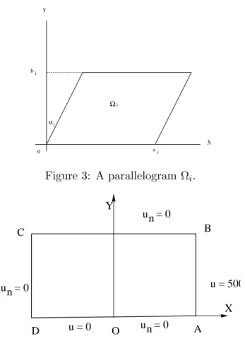
Proof : Consider the parallelograms Ωi in Figure 3, where ai and bi are the lengths of two edges, and αi are the angles between Ωi and the y axis. From the quasiuniform parallelograms,
where exist the bounds,
0 < ai, bi< C,
max{ai, bi}
min{ai, bi} ≤ C, 0 ≤ αi≤ αM <
π
2. (5.14) The parallelograms Ωican be transformed to 2 by the linear transformation T : (x, y) −→ (ˆx, ˆy),
where ˆ x = 2 ai(x − (tan αi)y) − 1, ˆ y = 2 biy − 1. Denote ˆw = T (w). We have ∂w ∂x = 2 ai ∂ ˆw ∂ ˆx, ∂w ∂y = − 2 ai(tan αi) ∂ ˆw ∂ ˆx + 2 bi ∂ ˆw ∂ ˆy.
Through the linear transformations T , we obtain
|w|21,Ωi = Z Z Ωi (wx2+ w2y)dxdy (5.15) = aibi 4 Z Z 2{( 2 ai ∂ ˆw ∂ ˆx) 2+ (−2 ai(tan αi) ∂ ˆw ∂ ˆx + 2 bi ∂ ˆw ∂ ˆy) 2}dˆxdˆy ≤ aibi 4 Z Z 2{ 4 a2 i (1 + 2 tan2αi)(∂ ˆw ∂ ˆx) 2+ 24 b2 i (∂ ˆw ∂ ˆy) 2}dˆxdˆy ≤ C Z Z 2{( ∂ ˆw ∂ ˆx) 2+ (∂ ˆw ∂ ˆy) 2}dˆxdˆy,
where the constant
C = max i { bi ai(1 + 2 tan 2α i) +2abi i }.
The constant C is independent of i due to assumption (5.14). Under the linear transformation
T , the polynomials of order L remain as well. Based on Lemma 5.3, we have for w = wL.
Z Z 2{( ∂ ˆw ∂ ˆx) 2+ (∂ ˆw ∂ ˆy) 2}dˆxdˆy ≤ CL4 Z Z 2( ˆw) 2dˆxdˆy. (5.16)
Moreover, through the inverse transformation ˆT , we obtain for w = wL
Z Z 2( ˆw) 2dˆxdˆy = 4 aibi Z Z Ωi w2dxdy ≤ Ckwk20,Ωi. (5.17)
Combining (5.15) and (5.17) gives |w|1,Ωi ≤ CL 2kwk 0,Ωi, and kwk1,Ωi ≤ CL 2kwk 0,Ωi.
Consequently, for parallelograms Ωi we have
kwLkk,Ωi ≤ C(L − k)2kwLkk−1,Ωi ≤ CL2kwLkk−1,Ωi ≤ CL 2kkw Lk0,Ωi. From A9 we obtain kwLk2k,S ≤X i kwLk2k,Ωi ≤ CL4kX i kwLk20,Ωi ≤ CL4kkwLk20,S,
by noting finite overlaps of Ωi. This completes the proof of Theorem 5.1.
6
Numerical Experiments
In the section, we carry out three computational models by using the collocation method.
6.1 Radial Basis Functions for Different Boundary Conditions
When the radial basis functions are chosen as the admissible functions, the analysis (in particu-lar the inverse inequalities) is made in Hu, Li and Cheng [12]. Here, we only provide numerical experiments, to show the effectiveness of the CM in this paper. Details of the rationale of radial basis functions, we refer the reader to [15, 16].
First, we consider the Poisson’s equation on domain S with the mixed type of boundary conditions
−∆u = 2π2sin(πx) cos(πy), in S, (6.1)
u = 0 on x = 1 ∧ 0 ≤ y ≤ 1, (6.2)
ux+ 2u = −π cos(πy) on x = −1 ∧ 0 ≤ y ≤ 1,
uy = 0 on y = 1 ∧ − 1 ≤ x ≤ 1,
u = sin(πx) on y = 0 ∧ − 1 ≤ x ≤ 1.
where S is a rectangle, S = {(x, y)| − 1 ≤ x ≤ 1, 0 ≤ y ≤ 1}, ∂S is its boundary, un= ∂u∂n, and
n is the outnormal to ∂S. Choose the solution
The purpose of the problem is to apply the collocation methods using the radial basis functions for different boundary conditions.
The admissible functions are chosen as:
v =
NS
X
i=1
aigi(x, y), in S, (6.4)
where ai are unknown coefficients to be determined, and gi(x, y) are the radial basis function.
First, we choose the inverse multiquadric radial basis functions (IMQRB)
gi(x, y) = q 1
r2
i + c2
, (6.5)
where c is a parameter constant, ri= {(x − xi)2+ (y − yi)2} 1
2, and (xi, yi) are the source points
which may not be necessarily chosen as the collocation nodes. Suitable additional functions may be added into (6.4), such as some polynomials and the singular functions if necessary. Next, we may choose the Gaussian radial basis functions (GRB)
gi(x, y) = exp à −ri2 c2 ! . (6.6)
We use the collocation equations (4.12)–(4.14) on the uniform interior collocation nodes, and choose the trapezoidal rules for (4.9)–(4.11). The error norms are listed in Tables 1 and 2 for IMQRB and GRB, respectively, where Nd denotes the number of partition along the y-direction in S. Let the source points of radial basis functions also be the collocation nodes. And let NS = L2 in (6.4). From Table 1, we can see the following asymptotic relations for
IMQRB
ku − vk0,∞,S= O((0.16)L), (6.7)
ku − vk0,S= O((0.17)L), (6.8)
ku − vk1,S= O((0.19)L). (6.9)
And from Table 2 we can see for GRB,
ku − vk0,∞,S= O((0.15)L), (6.10) ku − vk0,S= O((0.14)L), (6.11) ku − vk1,S= O((0.16)L). (6.12)
Eqs. (6.7)–(6.12) indicate that the numerical solutions have the exponential convergence rates. Note that the GRB collocation method converges slightly faster than the IMQRB collocation method.
6.2 Piecewise Admissible Functions
Next, consider the Poisson’s equation, ∆u = ∂2u
∂x2 + ∂2u
∂y2 = 0, in S, (6.13)
where S = {(x, y)| − 1 < x < 1, 0 < y < 1}, with the following boundary conditions:
u = cos(πy) on x = −1 ∧ 0 ≤ y ≤ 1, (6.14)
u = cosh(2π) cos(πy) on x = 1 ∧ 0 ≤ y ≤ 1,
u = − cosh((x + 1)π) on y = 1 ∧ − 1 ≤ x ≤ 1, uy = 0 on y = 0 ∧ − 1 ≤ x ≤ 1.
u+= u−, u+ν = u−ν on Γ0.
The exact solution is u(x, y) = cosh(π(x + 1)) cos(πy). Divide S into S1 and S2, where S1 = {(x, y)| − 1 < x < 0, 0 < y < 1} and S2 = {(x, y)|0 < x < 1, 0 < y < 1}. The admissible
functions are chosen as:
v = v−= XL i,j=0 aijTi(2x + 1)Tj(2y − 1), in S1 v+= XM i,j=0 dijTi(2x − 1)Tj(2y − 1), in S2 (6.15)
where aij and dij are unknown coefficients to be determined, and Ti(x) are the Chebyshev polynomials Tk(x) = cos(k cos−1(x)).
Then, we use the collocation equations, (2.28)–(2.32), and choose the trapezoidal rules for (2.24). Since v± do not satisfy the boundary conditions, some additional collocation v±(P
i) =
0, Pi∈ ∂S, are also needed. The error norms are listed in Table 3, the different expansion terms L and M are used in S1 and S2, respectively, and N is the number of collocation nodes along
y-axis in a uniform distribution. The following asymptotic relations are observed:
ku − v−k0,∞,S1 = O((0.161)L), ku − v+k0,∞,S2 = O((0.161)M), (6.16)
ku − v−k0,S1 = O((0.166)L), ku − v+k0,S2 = O((0.166)M), (6.17)
ku − v−k1,S1 = O((0.159)L), ku − v+k1,S2 = O((0.157)M), (6.18)
kε+− ε−k0,Γ0 = O((0.121)LM), Cond.(A) = O((1.78)LM), (6.19)
where LM = max {L, M }. Above equations indicate that the numerical solutions satisfy (2.8), to have justified the analysis in Section 3.
6.3 Motz’s Problem
Finally, consider the Motz’s problem, ∆u = ∂
2u ∂x2 +
∂2u
where S = {(x, y)|−1 < x < 1, 0 < y < 1}, with the following mixed type of Dirichlet-Neumann conditions, see Figure 4:
ux = 0 on x = −1 ∧ 0 ≤ y ≤ 1, (6.21)
u = 500 on x = 1 ∧ 0 ≤ y ≤ 1,
uy = 0 on y = 1 ∧ − 1 ≤ x ≤ 1,
u = 0 on y = 0 ∧ − 1 ≤ x < 0, uy = 0 on y = 0 ∧ 0 < x ≤ 1.
The origin (0, 0) is a singular point, since the solution behaviour is u = O(r12) as r → 0 due to
the intersection of the Dirichlet and Neumann conditions. The admissible functions are chosen as:
v = L X `=0 ˜ D`r`+ 1 2 cos(` + 1 2)θ, (6.22)
where ˜D` are unknown coefficients to be determined, and (r, θ) are the polar coordinates with
origin (0, 0). Note that the particular solutions r`+12 cos(` +1
2)θ satisfy (6.20) and the boundary
conditions exactly:
u = 0 on y = 0 ∧ − 1 ≤ x < 0, (6.23)
uy = 0 on y = 0 ∧ 0 < x ≤ 1. (6.24)
The unknown coefficients ˜D` in (6.22) can be determined by satisfying the rest boundary
conditions.
Denote by Vh the finite dimensional collocation of (6.22). Then the CM can be denoted by:
To seek uL such that
I(uL) = min v∈Vh I(v), (6.25) where I(v) = Z AB(v − 500) 2+ w2 1 Z BCv 2 ν + w21 Z CDv 2 ν, (6.26) with w1= 1 L. Denote k²kB= ku − uLkB = q I(u − uL) = q I(v). (6.27)
Then, we use the collocation equations only on the rest of the boundary,
√
αi(v − 500)(Qi) = 0, Qi on x = 1 ∧ 0 ≤ y ≤ 1, (6.28)
w1√αivν(Qi) = 0, Qi on x = −1 ∧ 0 ≤ y ≤ 1, (6.29)
where Qi and αi are the nodes and weights of some integral rules. Note that the equations (6.28)–(6.30) are just the boundary approximation method(BAM) in [14], which is a special case of the CM in this paper. Also note that the collocation nodes Qi in (6.28)-(6.30) are far
from the singular origin.
Denote by N the collocation number of ∂S along axis Y , the total number of all collocation nodes are 4N . First, choose the centroid rule, errors of the solutions from the BAM and condition number are listed in Tables 4 and 5. Moreover, choose the Gaussian rule with six nodes and the Gaussian rules with 1,2,4,6,8 and 10 nodes, the results are listed in Tables 6 and 7, and the best leading coefficients in Table 8 by the Gaussian rule with six nodes as L = 34 and N = 30.
For the centroid rule, the number of collocation nodes should be large enough to guarantee the uniformly Vh− elliptic inequality. There is no effects for reducing the the errors k²kB and
k²k∞,AB. It can be seen from Table 5 that N should be chosen as N ≥ L2 for L = 34. From Table 7, we also conclude that the Gaussian rules of high order do not reduce the errors k²kB, but do improve accuracy of leading coefficients. For L = 34 and N = 30, the exact leading coefficients ˜D0 is obtained by the Gaussian rule of six nodes, see Table 8,
˜
D0= 401.162453745234416 (6.31)
Compared (6.31) with more accurate value [13] using higher precision by Mathematica, the relative error is less than the rounding error of double precision! This implies that ˜D0 in (6.31)
has 17 decimal significant digits.
To close this section, let us first comment the assumptions A1 and A2, then the numerical stability.
Remark 6.1 Usually, the solution of (2.1)-(2.3) is highly smooth inside of S, but less smooth on ∂S. In particular, for concave corners of polygons or the intersection points of the Dirichlet and Neumann boundary conditions, the solution is singular with infinite derivatives. In this case, some special treatments should be solicited. For Motz’s problem with th singular point at the origin in Section 6.3, the collocation equations are established at the nodes Qi far
from the singular origin, see (6.28)-(6.30). Hence assumptions A2 may be relaxed to
v±∈ H1(S) ∩ C2(D),
where D ⊂⊂ S. Moreover, when the singular functions or singular particular solution v± are
chosen, assumption A3 may also hold.
Remark 6.2 In real computation, the over-determined equations (2.33) are solved, which involve only the second and first order derivatives of the solutions respectively. It is well known that the condition number of the spectral methods and the collocation methods defined in (2.35) is large, also see Tables 1-7. To improve the number stability, we may invoke the preconditioner approaches. In real computation, however, the very accurate solution and the leading coefficient
˜
D0 in (6.31) with 17 significant digits have been achieved.
There arises a puzzle that the Cond. is large, while the solutions and ˜D0 are extremely
[7] and Christiansen and Hansen [8]. In fact, the definitions of Cond. by (2.35) occur only at the worst cases where the solution and the permutation are just equal to the eigenfunctions of the maximal and minimal eigenvalues for the stiffness matrix. These cases will not happen for the Motz’s solutions. Let us take (2.16) as an example. Suppose that matrix F is decomposed as [7, 8],
F = UΣV, (6.32)
where U and V are two orthogonal matrices, and Σ is the diagonal matrix with the declined singular values
σ1 ≥ σ2≥ ... ≥ σn> 0. (6.33) Let βi = ~uiT~b, where the vectors ~ui are given by U = ( ~u1, ..., ~un). Then the effect condition
number can be defined from [7, 8],
Cond eff = 1 σn q β2 1 + ... + βn2 q (β1 σ1) 2+ ... + (βn σn) 2. (6.34)
Obviously, when β2 = ... = βn = 0, Eq. (6.34) leads to the definition (2.35). Note that the
formulae in (6.34) is somehow different from that given in [8], but it is easily computed. Let us evaluated the Cond eff for the solution given in Table 8. The singular values σi of F and the coefficients βi are listed in Table 9. Based on Table 9, we obtain the two condition numbers
and their ratio,
Cond eff = 4.87, Cond. = 0.679(6), (6.35) Cond.
Cond eff = 0.139(6).
The fact that the effect condition number is less than 5 may explain very well the high accuracy of ˜D0 with 17 significant digits. In fact, from Table 9, for ~b (i.e., solution ~x), when the portion
of eigenfunction of σn ¯ β = q βn β2 1 + ... + βn2 = 27.017 155.035 = 0.174. (6.36) is not insignificant, the effect condition number is approximated from (6.34) by
Cond eff ≈ 1¯
β =
1
0.174 = 5.74, (6.37) which is still small. The above arguments are also valid for the collocation methods in Sections 6.1 and 6.2.
7
Finial Remarks
1. In this paper, the collocation method is treated as the least squares method, involving integration approximation. We employ the FEM theory to develop the theoretical analysis of CMs, in which the key analysis for combination of CMs is to prove the new Vh− elliptic
inequality.
2. Three typical boundary conditions, Dirichlet, Neumann and Robin, can be handled well by the techniques of CM in this paper. The number of collocation nodes may be chosen to be much larger than the number of radial basis functions(i.e., source points). The collocation nodes are, indeed, the integration nodes of the rules used. Based on integration approximation, not only can the collocation nodes be easily located, but also the error analysis has been developed, see Sections 2 and 3.
3. Three computational examples in Section 6 show exponentially convergent rates: ku −
vkk,S = O(λL), k = 0, 1, 0 < λ < 1, which verify perfectly the analysis made. Section 6.1
displays that the CM can be applied to many kinds of admissible functions, such as radial basis functions. The detailed analysis is given in Hu, Li and Cheng [12].
4. Piecewise admissible functions can be used in the CM, both the analysis and computation are provided in this paper. This enables the CM to be more flexible to complicated geometric domains for general PDEs, because different admissible functions can be chosen in different subdomains. Such an idea is also similar to the p−version of Babuˇska and Guo [2], and the analysis of the CM may also be extended to singularity problems by following [2].
5. From Remarks 6.1 and 6.2, the explanation of assumptions A2 and A3 and effect condition number may explain well the good computational results in many reports and our numerical experiments.
6. The BAM in [13, 14] is a special case of the CM in this paper. The numerical results of Section 6.3 are better than those in [13, 14]. The Gaussian rules with high orders are used to raise the accuracy of the leading coefficient D0 obtained by the BAM. ˜D0 in (6.31) is exact,
in the sense of the errors less than the rounding errors of double precision, compared with the more accurate value of ˜D0 in [13]. This new discovery will change the evaluation of the BAM
given in [13], where, based on the numerical results in [14] using the centroid rule, “BAM may
produce the best global solutions”, and “the conformal transformation method(CTM) is the most accurate method for leading coefficients”, see [13], p.133. Now we may conclude that for Motz’s
problem, the BAM (by the Gaussian rule with six nodes) is the most accurate method not only in the global solutions but also in the leading coefficient, ˜D0.
Acknowledgments
References
[1] D. N. Arnold and W. L. Wendland, On the asymptotic convergence of collocation method, Math. Comp., Vol. 41, No.164, pp.349-381, 1983.
[2] I. Babuˇska and B. Guo, Direct and inverse approximation theorems for the p-version of the
finite element method is the framework of weighted Besov spaces, Part III: Inverse approx-imation theorems, Technical Report, Department of Mathematics, University of Manitoba,
2002.
[3] C. Bernardi, N. Debit and Y. Maday, Coupling finite element and spectral methods: First
result, Math. Comp., Vol. 54, pp.21-39, 1990.
[4] C. Bernardi and Y. Maday, Spectral methods in techniques of scientific computing (Part 2), Handbook of Numerical Analysis, Vol. V (Edited by P. G. Ciarlet and J. L. Lions), Elsevier Science, 1997.
[5] C. Canuto, S. I. Hariharan and L. Lustman, Spectral methods for exterior elliptic problems, Numer Math. Vol. 46, pp.505-520, 1985.
[6] C. Canuto, M. Y. Hussaini, A. Quarteroni and T. A. Zang, Spectral Methods in Fluid Dynamics, Springer-Verlag, New York, 1987.
[7] T. F. Chan and D. Foulser, Effectively well-conditioned linear systems, SIAM J. Sci, Stat. Comput., Vol. 9, pp. 963-969, 1988.
[8] S. Christiansen and P. C. Hansen, The effective condition applied to error analysis of
certain boundary collocation methods, J. Comput. Appl. Math., Vol. 54, pp. 1-34, 1994.
[9] P. G. Ciarlet, Basic error estimates for elliptic problems, in Eds., P.G. Ciarlet and J. L. Lions, Finite Element Methods (Part I), p. 17-352, North-Holland, 1991.
[10] G. H. Golub and C. F. Loan, Matrix Computations (Sec Ed.), Chaps. 3,4,12, The Johns Hopkins University Press, Baltimore and London, 1989.
[11] D. Gottlieb and S. A. Orszag, Numerical Analysis of Spectral Methods: Theory and Applications, SIAM, Philadelphia, 1977.
[12] H. Y. Hu, Z. C. Li and A. H. C. Cheng, Radial Basis Collocation Method for Elliptic
Boundary Value Problem, Computers & Mathemtaics with Application, to appear.
[13] Z. C. Li, Combined Methods for Elliptic Equations with Singularities, Interfaces and Infinities, Kluwer Academic Publishers, Boston, London, 1998.
[14] Z. C. Li, R. Mathon, and P. Sermer Boundary methods for solving elliptic problem with
singularities and interfaces, SIAM J. Numer. Anal., Vol. 24, pp.487-498, 1987.
[15] W. R. Madych, Miscellaneous error bounds for multiquadric and related interpolatory, Computers & Mathematics with Application, Vol. 24, No.12, pp.121-138, 1992.
[16] W. R. Madych and S. A. Nelson, Multivariate interpolation and conditionally positive
definite functions, I., Math. Comp. Vol. 54, pp. 211-230, 1990.
[17] B. Mercier, Numerical Analysis of Spectral Method, Springer-Verlag, Berlin, 1989. [18] D. Pathria and G. E. Karniadakis, Spectral element methods for Elliptic problems in
non-smooth domains, J. Comput. Phys. Vol. 122, pp.83-95, 1995.
[19] A. Quarteroni and A. Valli, Numerical Approximation of Partial Differential Equa-tion, Springer-Verlag, Berlin, 1994.
[20] J. Shen, Efficient Spectral-Galerkin method I. Direct solvers of second- and fourth- order
equations using Legendre polynomials, SIAM. J. Sci. Comput., Vol. 14, pp.1489-1505, 1994.
[21] J. Shen, Efficient Spectral-Galerkin method II. Direct solvers of second- and fourth- order
equations using Chebyshev polynomials, SIAM. J. Sci. Comput., Vol. 15, pp.74-87, 1995.
[22] J. Shen, Efficient Spectral-Galerkin method III. Polar and cylindrical geometries, SIAM. J. Sci. Comput., Vol. 18, pp.1583-1604, 1997.
[23] G. E. Sneddon, Second-order spectral differentiation matrices, SIAM J. Numer. Anal. Vol. 33, pp.2468-2487, 1996.
[24] G. Strang and G. J. Fix, An Analysis of the Finite Element Method, Prentice-Hall, 1973.
[25] G. Yin, Sinc-Collocation method with orthogonalization for singular Poisson-like problems, Math. Comp., Vol. 62, No. 205, pp.21-40, 1994.
Γ 0 1 S 2 S
Figure 1: Partition of a convex polygon.
2 5 Ω Ω Ω Ω Ω3 4 1
0 a b i i i X Y αi Ω Figure 3: A parallelogram Ωi. X u = 500 B u = 0 A u = 0 O n u = 0 D u = 0 C Y n n
Figure 4: Motz’s problem Table 1.
The error norms and condition number by the inverse multiquadric radial basis collocation method with parameter c = 2.0.
Nd, L 16, 4 16, 6 16, 8 16, 10
ku − vk0,∞,S 1.72 7.27(-2) 5.28(-4) 2.78(-5)
ku − vk0,S 4.83(-1) 2.21(-2) 8.87(-5) 1.26(-5)
ku − vk1,S 2.02 9.09(-2) 9.48(-4) 8.16(-5) Cond.(A) 2.00(3) 6.36(5) 3.81(8) 1.39(9)
Table 2.
The error norms and condition number by the Gaussian radial basis collocation method with parameter c = 2.0. Nd, L 16, 4 16, 6 16, 8 16, 10 ku − vk0,∞,S 1.53 8.25(-2) 7.46(-4) 1.37(-5) ku − vk0,S 4.80(-1) 2.43(-2) 1.60(-4) 3.44(-6) ku − vk1,S 1.92 1.15(-1) 1.30(-3) 3.65(-5) Cond.(A) 1.08(4) 1.53(8) 1.05(9) 3.69(9) Table 3.
The error norms and condition number by Combination of CM with the different expansion terms L and M used in S1 and S2, respectively, and the number N of collocation nodes along
y-axis in a uniform distribution.
L, M, N 3, 5, 6 4, 6, 8 5, 7, 10 6, 8, 12 7, 9, 14 ku − v−k 0,∞,S1 3.41(-1) 1.39(-1) 9.23(-3) 1.86(-3) 2.29(-4) ku − v−k 0,S1 6.92(-2) 3.75(-2) 2.12(-3) 4.54(-4) 5.31(-5) ku − v−k 1,S1 5.23(-1) 1.85(-1) 1.69(-2) 3.82(-3) 3.33(-4) ku − v+k 0,∞,S2 3.09(-1) 1.46(-1) 8.15(-3) 1.83(-3) 2.06(-4) ku − v+k 0,S2 6.26(-2) 3.59(-2) 1.91(-3) 3.59(-4) 4.72(-5) ku − v+k 1,S2 4.74(-1) 1.74(-1) 1.43(-2) 3.30(-3) 2.86(-4) kε+− ε−k 0,Γ0 1.23(-3) 9.34(-4) 1.56(-5) 8.59(-6) 2.64(-7) Cond.(A) 7.96(2) 1.52(3) 2.82(3) 4.82(3) 7.80(3)
Table 4.
The error norms and condition number by the BAM with centroid rule. L N kεkB |ε|∞, ¯AB Cond.(A) |4DD00| | 4D1 D1 | | 4D2 D2 | | 4D3 D3 | 10 8 0.250(-1) 0.149(-1) 94.3 0.189(-5) 0.491(-5) 0.601(-5) 0.928(-3) 18 12 0.133(-3) 0.811(-4) 0.193(4) 0.158(-7) 0.113(-6) 0.290(-6) 0.502(-6) 26 16 0.973(-6) 0.734(-6) 0.366(5) 0.216(-9) 0.155(-8) 0.380(-8) 0.202(-8) 34 24 0.839(-8) 0.459(-8) 0.666(6) 0.169(-11) 0.121(-10) 0.296(-10) 0.152(-10) Table 5.
The error norms and condition number by the BAM with the centroid rule as L = 34. N kεkB |ε|∞, ¯AB Cond.(A) |4DD00| | 4D1 D1 | | 4D2 D2 | | 4D3 D3 | 9 0.135(-8) 0.496(-6) 0.267(8) 0.377(-9) 0.266(-8) 0.641(-8) 0.342(-8) 12 0.587(-8) 0.713(-7) 0.992(6) 0.337(-10) 0.239(-9) 0.578(-9) 0.305(-9) 16 0.772(-8) 0.189(-7) 0.679(6) 0.729(-11) 0.520(-10) 0.127(-9) 0.655(-10) 24 0.839(-8) 0.459(-8) 0.669(6) 0.169(-11) 0.121(-16) 0.296(-10) 0.152(-10) 32 0.849(-8) 0.462(-8) 0.669(6) 0.769(-11) 0.550(-11) 0.134(-10) 0.695(-11) Table 6.
The error norms and condition number by the BAM for L = 34 using the Gaussian rule with six nodes. N kεkB |ε|∞, ¯AB Cond.(A) |4DD00| | 4D1 D1 | | 4D2 D2 | | 4D3 D3 | 12 0.359(-8) 0.721(-8) 0.675(6) 0.531(-13) 0.646(-12) 0.405(-11) 0.868(-11) 18 0.494(-8) 0.629(-8) 0.679(6) 0.468(-14) 0.211(-14) 0.620(-13) 0.352(-14) 24 0.491(-8) 0.530(-8) 0.679(6) 0.567(-15) 0.324(-15) 0.103(-14) 0.337(-13) 30 0.493(-8) 0.520(-8) 0.676(6) 0∗ 0.162(-15) 0.124(-14) 0.317(-13) 36 0.494(-8) 0.520(-8) 0.679(6) 0.850(-15) 0.324(-15) 0.103(-14) 0.308(-13)
∗ The error less then computer rounding errors in double precision. Table 7.
The error norms and condition number by BAM with different Gaussian rules as L = 34. Rule N kεkB |ε|∞, ¯AB Cond.(A) |4DD00| | 4D1 D1 | | 4D2 D2 | | 4D3 D3 | Gauss(1) 24 0.839(-8) 0.459(-8) 0.606(6) 0.169(-11) 0.121(-10) 0.296(-10) 0.152(-10) Gauss(2) 24 0.854(-8) 0.369(-8) 0.672(6) 0.708(-13) 0.512(-12) 0.133(-11) 0.106(-11) Gauss(4) 24 0.610(-8) 0.540(-8) 0.679(6) 0.425(-15) 0.535(-14) 0.641(-13) 0.755(-13) Gauss(6) 30 0.493(-8) 0.520(-8) 0.676(6) 0∗ 0.162(-15) 0.124(-14) 0.317(-13) Gauss(8) 24 0.428(-8) 0.519(-8) 0.679(6) 0.142(-15) 0.648(-15) 0.618(-15) 0.315(-13) Gauss(10) 20 0.639(-8) 0.521(-8) 0.679(6) 0.142(-15) 0∗ 0.412(-15) 0.308(-13)
Table 8.
The leading coefficients by the BAM with Gaussian rule of six as L = 34 and N = 30.
` D˜` 0 401.162453745234416 1 87.6559201950879299 2 17.2379150794467897 3 -8.0712152596987790 4 1.44027271702238968 5 0.331054885920006037 6 0.275437344507860671 7 -0.869329945041107943(-1) 8 0.336048784027428854(-1) 9 0.153843744594011413(-1) 10 0.730230164737157971(-2) 11 -0.318411361654662899(-2) 12 0.122064586154974736(-2) 13 0.530965295822850803(-3) 14 0.271512022889081647(-3) 15 -0.120045043773287966(-3) 16 0.505389241414919585(-4) 17 0.231662561135488172(-4) 18 0.115348467265589439(-4) 19 -0.529323807785491411(-5) 20 0.228975882995988624(-5) 21 0.106239406374917051(-5) 22 0.530725263258556923(-6) 23 -0.245074785537844696(-6) 24 0.108644983229739802(-6) 25 0.510347415146524412(-7) 26 0.254050384217598898(-7) 27 -0.110464929421918792(-7) 28 0.493426255784041972(-8) 29 0.232829745036186828(-8) 30 0.115208023942516515(-8) 31 -0.345561696019388690(-9) 32 0.153086899837533823(-9) 33 0.722770554189099639(-10) 34 0.352933005315648864(-10)
Table 9.
The singular values σiand the coefficients βi for the matrix resulting from the collation Trefftz method for Motz’s problem at N = 34 by the Gaussian rule of six nodes with M = 30 along AB, where the
Cond. = 0.679(6) and Cond eff=4.87.
i σi βi i σi βi 0 .158(5) -29.079 18 .156(1) -10.439 1 .121(5) -37.122 19 .126(1) 13.978 2 .846(4) -25.088 20 .113(1) .925 3 .595(4) 32.111 21 .974 -17.143 4 .558(3) 27.281 22 .827 -31.730 5 .386(3) -1.639 23 .720 -37.569 6 .269(3) -7.219 24 .677 42.050 7 .195(3) -9.980 25 .560 17.276 8 .513(2) .391 26 .463 1.684 9 .345(2) -31.549 27 .368 -12.385 10 .249(2) -38.967 28 .305 9.257 11 .189(2) -20.462 29 .249 19.718 12 .931(1) -13.804 30 .188 6.208 13 .619(1) -37.104 31 .141 -36.807 14 .470(1) -31.307 32 .102 -44.190 15 .381(1) 43.315 33 .556(-1) 27.483 16 .267(1) 33.821 34 .233(-1) 27.017 17 .202(1) 14.385 / / /