Constructing the maximum consensus tree from rooted triples

全文

(1)Jú65ÈíÉ[ |×ø_4ííc. Constructing the maximum consensus tree from rooted triples Økø(Bang Ye Wu) c,x×ç’m ˙Í Email:bangye@mail.stu.edu.tw. Abstract We investigated the problem of constructing the maximum consensus tree from rooted triples. We showed the NP-hardness of the problem and developed exact and heuristic algorithms. The exact algorithm is based on the dynamic programming strategy and runs in O((m + n2 )3n ) time and O(2n ) space. The heuristic algorithms were tested and their performances are shown by comparing with the optimal solutions. The experimental results show that the worst and average case relative error ratios are 1.214 and 1.075 respectively, which are much better than the previously best approximation ratio of the problem. Keywords: computational biology, evolutionary trees, algorithms, dynamic programming, NP-hardness. 1. Introduction. Evolutionary trees are used to present the relationship among a set of species. The leaves in an evolutionary tree correspond to the species and internal nodes are the ancestors of the species. Constructing evolutionary trees is an important problem in computational biology and there are different approaches. We investigated the problem of constructing evolutionary trees from rooted triples. A rooted triple, or triple for brevity, represents the relationship of three species. As shown in Figure 1, a triple (a(bc)) specifies lca(a, b) = lca(a, c) > lca(b, c), in which lca(a, b) is the lowest common ancestor of the two leaves and relation ”>” means ”is an ancestor of ”. For a set of triples, the exact consensus tree is the tree satisfies all given triples. Given a set of triples, the existence of the. exact consensus tree can be determined in polynomial time [1]. For a set of constraints of the form lca(a, b) > lca(c, d), the algorithm in [1] determines if there is a tree satisfying all constraints and finds such a tree if it exists. A triple (a(bc)) is equivalent to lca(a, c) > lca(b, c) and is a special case of the constraints considered in [1]. An algorithm for constructing all exact consensus trees from triples was also developed [5]. Unfortunately, it is often impossible to find the exact consensus tree and we want to find the tree satisfying as many given triples as possible. We shall call the optimization problem the maximum consensus tree from rooted triples problem, or the MCTT problem for brevity. In [3], the problem to find the maximum consensus tree from constraints of the form lca(a, b) > lca(c, d) was shown to be NPhard and a 3-approximation algorithm was proposed. The approximation algorithm also works for the MCTT problem but the complexity of the MCTT problem was left open. Similar problems for unrooted trees were also investigated. A quartet represents the relationship of four species. To determine if there is a tree satisfying a given set of quartets were shown to be NP-complete [6]. Therefore the corresponding optimization problem is obviously NP-hard. In this paper, we show that the MCTT problem is NP-hard. Exact and heuristic algorithms are also presented. The exact algorithm is based on the dynamic programming strategy and runs in O((m + n2 )3n ) time and O(2n ) space. The performances of the heuristic algorithms were tested by comparing their outputs with the exact solutions. The experimental results show that the worst and average case relative error ratios are 1.214 and 1.075 respectively, which are much better than the previously best approximation ratio.

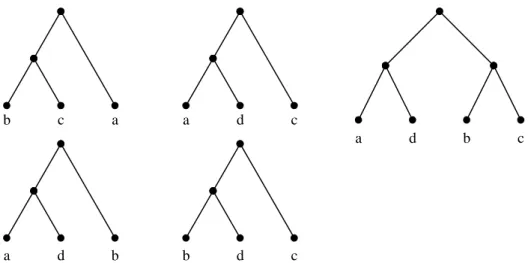
(2) b. c. a. a. d. c a. a. d. b. b. d. d. b. c. c. Figure 1: Left: rooted triples (a(bc)), (c(ad)), (b(ad)), (c(bd)); Right: the maximum consensus tree. The tree satisfies all triples except (c(bd)).. of the problem [3]. The time complexity of the MCTT problem is shown in Section 2. In Section 3, we present the exact and heuristic algorithms and the experimental results. We give a discussion in Section 4.. 2. The computational complexity. In this section, we shall show the NP-hardness of the MCTT problem by reducing the Feedback Arc Set problem to it. We first give the definition of the Feedback Arc Set problem. Definition 1: Let G = (V, A) be a directed graph. A subset A0 of A is a feedback arc set if every directed cycle in G contains at least one arc in A0 . Given a directed graph G = (V, A) and an integer k, the Feedback Arc Set problem asks if there is a feedback arc set A0 with |A0 | ≤ k. The Feedback Arc Set problem is NPcomplete [4, 2]. Definition 2: Let a and b be nodes of a tree. The lowest common ancestor of a and b is denoted by lca(a, b). We write a > b if a is an ancestor of b. Definition 3 : A rooted triple, or triple for brevity, over a species set is a constraint on the relationship of three species. Let V be a species set and a, b, c ∈ V , the rooted. triple (a(bc)) over V represents lca(a, b) = lca(a, c) > lca(b, c) in the desired tree. We say that a tree satisfies a triple or a triple is compatible with a tree if the relationship represented by the triple is satisfied in the tree. Definition 4 : Given a set Y of rooted triples over leaf set V , the maximum consensus tree from triples (MCTT) problem looks for a binary tree T with leaf set V such that the number of triples compatible with T is maximum. The computational complexity is shown in the next theorem. Theorem 1: hard.. The MCTT problem is NP-. Proof: We reduce the Feedback Arc Set problem to the MCTT problem. Given an instance G = (V, A) and k of the Feedback Arc Set problem, we shall construct a set of rooted triples Y and show that the directed graph G contains a feedback arc set of k arcs if and only if there is a tree compatible with |A| − k triples from Y . Let x ∈ / V . For every arc (u, v) ∈ A, there is a corresponding triple (u(xv)) in Y . Suppose that A0 is a feedback arc set of G and |A0 | = k . Since A0 is a feedback arc set, removing A0 from G results in a directed acyclic graph G1 = (V, A1 ), in which A1 = A \ A0 . Since G1 contains no cycle, we may assign.

(3) each vertex v a label f (v) ∈ {1 . . . p} such that f (u) < f (v) for every (u, v) ∈ A1 , where p ≤ |V | is number of nodes of the longest path in G1 . Let Vi = {v|f (v) = i} and Ti be an arbitrary evolutionary tree of Vi for 1 ≤ i ≤ p. We construct an evolutionary tree T of V ∪ {x} as in Figure 2. For any arc (u, v) ∈ A1 , since f (u) < f (v), the corresponding triple (u(xv)) in Y is compatible with T . Therefore all triples corresponding to arcs in A1 are satisfied, and T is compatible with |A| − k triples in Y . Conversely suppose that there is a tree T compatible with |A|−k triples in Y . Let Y1 be the set of satisfied triples in Y . As in Fig.2, let the path from root to x be (r1 , r2 , . . . , rp , x) and Vi denote the set of leaves whose common ancestor with x is ri . For each triple (u(xv)) ∈ Y1 in which u ∈ Vi and v ∈ Vj , since lca(u, x) = lca(u, v) > lca(x, v), we have j > i. Let A1 be the set of arcs corresponding to the triples in Y1 , that is A1 = {(u, v)|(u(xv)) ∈ Y1 }. Consider the graph G1 = (V, A1 ) and label each vertex v with i if v ∈ Vi . Since all the arcs in A1 are from vertices with small labels to larger labels, G1 contains no directed cycle. Therefore A \ A1 is a feedback arc set of G and contains k arcs. The above transformation reduces the Feedback Arc Set problem to the MCTT problem in polynomial time. Since the Feedback Arc Set problem is NP-complete, the MCTT problem is NP-hard.. 3. Algorithms and experimental results. In this section, exact and heuristic algorithms will be developed. In the remaining of this paper, Y is the set of the input triples over species set U . Let n and m be the cardinalities of U and Y respectively.. Definition 6 : Let V ⊂ U , the set of all bipartitions of V is denoted by B(V ). Definition 7: Let V ⊂ U and (V1 , V2 ) ∈ B(V ). We use w(V1 , V2 ) to denote the number of triples (x(v1 v2 )) in which v1 ∈ V1 , v2 ∈ V2 and x ∈ / V. The exact algorithm uses the dynamic programming strategy and is based on the following formula: score(V ) =. max. {score(V1 ). (V1 ,V2 )∈B(V ). +score(V2 ) + w(V1 , V2 )}. (1). Obviously score(U ) is the maximum number of satisfiable triples in Y . The exact algorithm is list below. Theorem 2 : The algorithm Exact MCTT computes the maximum consensus tree from rooted triples with time complexity O((m + n2 )3n ) and space O(2n ). Proof: The correctness of the algorithm is from Equation 1. The algorithm computes the scores of subsets with cardinalities from small to large. When computing the score of set V , the scores of all its subsets have been found. The storage space used by the algorithms is O(2n +m+n2 ), O(2n ) for the scores and partitions of all subsets and O(m+n2 ) for the triples. Since 2n is larger than m+n2 , the space complexity is O(2n ). For each bipartition (V1 , V2 ) of any subset, the time complexity for computing w(V1 , V2 ) is no more than n2 + m since there are totally m triples and O(n2 ) pairs (i, j) of species with i ∈ V1 and j ∈ V2 . Since there are 2k bipartitions ¡ ¢ for a set of cardinality k and there are nk subsets of U with cardinality k, the time complexity is µ ¶ n X 2 k n = (n2 + m)(1 + 2)n (n + m) 2 k k=1. = (n2 + m)3n. 3.1. An exact algorithm. In this subsection, we shall present an algorithm to find the exact solution of the MCTT problem.. 3.2. Definition 5: Let V ⊂ U , we use score(V ) to denote the maximum number of satisfiable triples in {(a(bc))| b, c ∈ V } ⊂ Y .. In this subsection, we shall present heuristic algorithms for the MCTT problem. The heuristic algorithms do not ensure the optimality of the found solutions but it runs in. Heuristic algorithms.

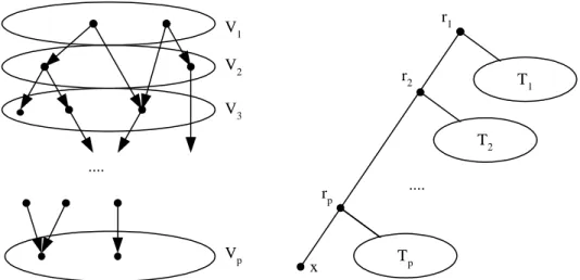
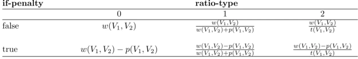
(4) r1. V1 V2. r2. T1. V3 T2 .... rp. Vp. x. ..... Tp. Figure 2: Transformation of an instance of the Feedback Arc Set problem into that of the MCTT problem. Left: the labeling of a directed acyclic graph; Right: A maximum consensus tree of the MCTT problem.. polynomial time. The performance of the heuristics will be shown by comparing with the optimal solutions found by the exact algorithm represented in the previous subsection. Our heuristic algorithms Best-PairMerge-First works as follows: Initially there are n subsets and each contains one of the species. The algorithms then repeatedly merge pair of subsets until there is only one set left. But it is a question to determine the two subsets to be merged at each iteration. We shall define a function e score(V1 , V2 ) to evaluate the score of merging sets V1 and V2 . At each iteration, the algorithm chooses the two sets with maximum evaluation score. To evaluate the score, an intuitive method is to choose sets V1 and V2 with maximum w(V1 , V2 ). That is, we greedily merge two sets which satisfy as many triples as possible. Besides the intuitive method, the following two points were also considered and the scoring function is depends on two parameters if-penalty and ratio-type. • Merging two sets not only satisfies some triples but also makes some triples unsatisfiable. Precisely speaking, merging V1 and V2 satisfies the triples (x(ij)) but conflicts with the triples (i(xj)) and (j(xi)), where i ∈ V1 , j ∈ V2 and x ∈ / V1 ∪ V2 . We define the penalty p(V1 , V2 ) as the number of triples conflicted by merging the two sets. When the input parameter if-penalty is true, the algorithm uses w(V1 , V2 ) − p(V1 , V2 ) to select. the two sets to be merged. Otherwise only w(V1 , V2 ) is considered.. • There may be bias to evaluate the subset pairs by the number of satisfied triples since the distribution of the triples may be not uniform and the cardinalities of the subsets are different while the program is running. Therefore it may be better to use relative score than the number of satisfied triples. Two ratios were considered in our algorithm. One is w(V1 , V2 )/(w(V1 , V2 ) + p(V1 , V2 )), and the other is w(V1 , V2 )/t(V1 , V2 ), in which t(V1 , V2 ) is the total number of triples (x(v1 v2 )) for all v1 ∈ V1 and v2 ∈ V2 . When the penalty is considered, the numerator is replaced with w(V1 , V2 ) − p(V1 , V2 ) in either ratio. A parameter ratio-type is used to determine which ratio will be used. If it is zero, the algorithm does not use the relative ratio.. The two parameters give us six scoring functions. The performance of all the alternatives were tested. The heuristic algorithm is listed below. For different combinations of the two parameter, the function e score is defined in Table 1..

(5) Algorithm Exact MCTT Input: A set Y of rooted triples over species set U . All triples are stored in a matrix M of lists. M [i, j] is a list of the elements of set {x|(x(ij)) ∈ Y }. Output: A rooted tree T satisfying maximum number of triples in Y . Step 1: Compute the maximum number of satisfied triples. For i=1 to n do For each subset V with cardinality i do For each bipartition (V1 , V2 ) of V do Compute w(V1 , V2 ) by counting the number of elements in M [i, j] \ V for each i ∈ V1 and j ∈ V2 ; score(V ) = max{score(V1 ) + score(V2 ) + w(V1 , V2 )}, in which the maximum is taken over all bipartitions of V . Record the best bipartition of V at P artition(V ). Step 2: Construct the tree by backtracking P artition(U ). Start with V = U . If V contains only one species, create a leaf node for it. Otherwise recursively construct trees T1 and T2 for V1 and V2 respectively, where (V1 , V2 ) is the best bipartition of V recorded at Step 1. Step 3: Output the tree.. Algorithm Best-Pair-Merge-First(if-penalty,ratio-type) Step 1: Initialization Let T = {Ti | 1 ≤ i ≤ n}, in which Ti is the tree contains only one leaf i. Step 2: Iteratively merging While there are more than one trees in T do Select two trees Ti and Tj in T such that e score(V (Ti ), V (Tj )) is maximum, in which e score(V (Ti ), V (Tj )) depends on the parameters if-penalty and ratio-type as defined in Table 1 ; Merge Ti and Tj by adding an common ancestor and replace Ti and Tj by the merged tree; Step 3: Output the tree in T .. 3.3 3.3.1. The experimental results The environment of the experiments. Both the exact and heuristic algorithms were coded in ANSI C and ported on a personal computer equiped with Intel Pentium III-733 CPU and 64M bytes memory. The platform is Microsoft WIN32. The triples were generated randomly over all species. 3.3.2. Running time. We tested the running time for the exact algorithm for n from 10 to 20. Since the algorithm uses the dynamic programming strategy. The. running time does not vary for different instances. For each n, three data instances were tested. The results are shown in Table 2. 3.3.3. Error ratios. The performances of the heuristic algorithms are shown in the following tables. Table 3 and 4 show the worst case ratios for different numbers of triples. For each case, 100 data were tested. The error ratio is obtained by opt(Y )/heu(A, Y ), where opt(Y ) is the maximum number of satisfiable triples in Y and heu(A, Y ) is the number of triples satisfied by the tree found by heuristic algorithm A. The last column labeled by Multiple is the.

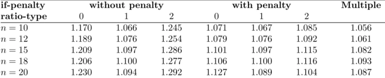
(6) Table 1: The evaluation score e score(V1 , V2 ) for combinations of parameters if-penalty ratio-type 0 1 2 w(V1 ,V2 ) w(V1 ,V2 ) false w(V1 , V2 ) w(V1 ,V2 )+p(V1 ,V2 ) t(V1 ,V2 ) true. w(V1 , V2 ) − p(V1 , V2 ). results for the algorithm which runs all the six heuristics and chooses the best for each data instance. Table 5 and 6 show the average and worst case ratios for different number of species. The number of the tests is 300 for n = 10, 12, 15, and 30 for n = 18, and 6 for n = 20.. 4. Discussion. In the following paragraphs, the heuristics will be referred as BPMF(p1 ,p2 ), in which the p1 and p2 are the input parameters. By the results of experiments, we observed the following: • By the results of individual data instances (not shown in the paper), we found that no one of the six heuristics is absolutely better than another. For each of them, there are some instances that it finds better solutions than all the others. This is also the reason why the heuristic Multiple performs better than all the others. • Taking penalty into consideration improves the performance significantly. Note that the evaluation score of BPMF(no-penalty,ratio-type=1) in fact involves the penalty. • Heuristics BPMF(no-penalty,ratiotype=1) and BPMF(penalty,ratiotype=1) perform very similarly. In over thousands of tests, there are only few cases that the scores of their outputs are different. • The error ratios are not sensitive to either the number of input triples or the number of species. We make some remarks as the conclusion. In most of the applications, the solution quality is the major concern. Therefore, for small data instances, the exact algorithm should be used. For large data instances, we propose. w(V1 ,V2 )−p(V1 ,V2 ) w(V1 ,V2 )+p(V1 ,V2 ). w(V1 ,V2 )−p(V1 ,V2 ) t(V1 ,V2 ). the heuristic Multiple since it takes the advantages of all the heuristics and runs in polynomial time. When the running time is an important factor, any one of the heuristics with penalty considered may be a good choice. There are also some open problems. We show the performances of the heuristics by experiments. It is interesting to give a theoretic analysis of the performance. The computational complexity of the MCTT problem is shown in this paper, but the approximability is still open.. Acknowledgements The work was partially supported by grant NSC 90-2213-E-366-005 from the National Science Council.. References [1] A.V. Aho, Y. Sagiv, T.G. Szymanski and J.D. Ullman, Inferring a tree from lowest common ancestors with an application to the optimization of relational expressions, SIAM Journal on Computing, vol. 10, no. 3, pp. 405–421, 1981. [2] M.R. Garey and D.S. Johnson, Computers and Intractability: A guide to the theory of NP-Completeness, W.H.Freeman and Company, San Fransisco, 1979. [3] L. Gasieniec, J. Jansson, A. Lingas and A. Ostlin, On the complexity of computing evolutionary trees, in Proceedings of the 3th Annual International Conference COCOON’97, pp.134–145, 1997. [4] R.M. Karp, Reducibility among combinatorial problems, in R.E. Miller and J.W. Thatcher (eds.) Complexity of Computer Computations, Plenum Press, New York, pp. 85–103, 1972..

(7) [5] M.P. Ng and N.C. Wormald, Reconstruction of rooted trees from subtrees, Discrete Applied Mathematics, vol. 69, pp. 19–31, 1996. [6] M. Steel, The complexity of reconstructing trees from qualitative characters and subtrees, Journal of Classification, vol. 9, pp. 91–116, 1992..

(8) n time in sec.. Table 2: The running time for Algorithm Exact MCTT 10 11 12 13 14 15 16 17 18 19 <1 1 2 9 30 104 366 1255 4322 14690. 20 49923. Table 3: The worst case error ratios for different number of triples with n = 10 if-penalty without penalty with penalty Multiple ratio-type 0 1 2 0 1 2 m = 60 1.455 1.200 1.523 1.214 1.200 1.321 1.192 m = 80 1.333 1.226 1.640 1.226 1.226 1.281 1.176 m = 100 1.424 1.175 1.551 1.194 1.189 1.285 1.150 m = 120 1.384 1.205 1.459 1.205 1.205 1.250 1.205. Table 4: The worst case error ratios for different number of triples with n = 15 if-penalty without penalty with penalty Multiple ratio-type 0 1 2 0 1 2 m = 100 1.538 1.208 1.579 1.208 1.208 1.250 1.208 m = 200 1.420 1.214 1.559 1.233 1.214 1.263 1.214 m = 300 1.264 1.132 1.452 1.152 1.132 1.164 1.132. if-penalty ratio-type n = 10 n = 12 n = 15 n = 18 n = 20. if-penalty ratio-type n = 10 n = 12 n = 15 n = 18 n = 20. Table 5: The average case error ratios for different number without penalty with penalty 0 1 2 0 1 1.170 1.066 1.245 1.071 1.067 1.189 1.076 1.254 1.079 1.076 1.209 1.097 1.286 1.101 1.097 1.206 1.100 1.277 1.106 1.100 1.230 1.094 1.292 1.127 1.089. of species Multiple 2 1.085 1.092 1.115 1.116 1.104. Table 6: The worst case error ratios for different number of species without penalty with penalty 0 1 2 0 1 2 1.455 1.226 1.640 1.226 1.226 1.321 1.486 1.293 1.576 1.293 1.293 1.325 1.538 1.214 1.579 1.233 1.214 1.263 1.343 1.237 1.435 1.190 1.237 1.221 1.288 1.125 1.372 1.145 1.116 1.142. 1.056 1.061 1.082 1.093 1.087. Multiple 1.205 1.178 1.214 1.190 1.116.

(9)